Abstract
This paper presents a novel method for locally estimating vehicle density on highways based on vehicle-to-vehicle (V2V) communication, a communication mode within intelligent transport systems (ITSs), enabled via IEEE 802.11p and 3GPP C-V2X technologies. Awareness messages (AMs), such as basic safety messages (BSMs, SAE J2735) and cooperative awareness messages (CAMs, ETSI EN 302 637-2), are periodically broadcast by vehicles and can be leveraged to sense the presence of nearby vehicles. Unlike existing approaches that directly combine the number of sensed vehicles with measured packet reception ratio (PRR) of the AM, our method accounts for the deviations in PRR caused by imperfect channel conditions. To address this, we estimate the actual packet reception probability (PRP)–distance curve by exploiting its inherent downward trend along with multiple measured PRR points. From this curve, two metrics are introduced: node awareness probability (NAP) and average awareness ratio (AAR), the latter representing the ratio of sensed vehicles to the total number of vehicles. The real density is then estimated using the number of sensed vehicles and AAR, mitigating the underestimation issues common in V2V-based methods. Simulation results across densities ranging from 0.02 vehs/m to 0.28 vehs/m demonstrate that our method improves estimation accuracy by up to 37% at an actual density of 0.28 vehs/m, compared with methods relying solely on received AMs, without introducing additional communication overhead. Additionally, we demonstrate a practical application where the basic safety message (BSM) transmission rate is dynamically adjusted based on the estimated density, thereby improving traffic management efficiency.
1. Introduction
1.1. Research Background
Traffic management is a complex task in the rapidly evolving transportation industry and expanding urban environments. Its primary objectives are to ensure safety, enhance efficiency, and promote sustainable environmental development [1,2]. Implementation is typically carried out within the framework of intelligent transport system (ITS), which encompasses applications such as congestion estimation, travel time prediction, traffic flow optimization, and dynamic routing [3]. The core parameters underlying these applications—vehicle speed (v), traffic flow (q), and vehicle density (k)—are interrelated through the fundamental diagram, [4,5]. According to this relationship, traffic control strategies can mitigate congestion, improve safety, and increase efficiency by maintaining vehicle density below a critical threshold [3]. For highway traffic management, Malekzadeh et al. [6] proposed a novel ramp metering approach for connected and automated vehicles (CAVs) in a lane-free traffic environment. In this method, vehicle density is a feedback parameter to dynamically adjust ramp vehicle speeds, keeping the mainstream density below the critical thresholds and thus preventing capacity drops at merge areas. Dynamic speed limit control operates on a similar principle, adjusting speed restrictions based on density to homogenize flow, minimize density fluctuations, and prevent congestion [3]. Network-level control approaches, such as model predictive control (MPC), optimize measures like ramp metering and variable speed limits by predicting density across the network to maximize overall throughput [3]. These approaches leverage density information to generate control signals that guide traffic toward stable states while preventing bottlenecks, congestion, and inefficient routing. Consequently, accurate vehicle density estimation remains a critical and ongoing challenge in traffic management.
Numerous vehicle density estimation methods have been proposed to determine vehicle counts. Early vehicle density estimation schemes relied on pre-installed cameras or sensors (including inductive loop detectors and roadside radars) to collect traffic data and estimate vehicle density [7]. These infrastructure-based methods have long been used in traffic engineering and continue to be refined to enhance estimation accuracy. However, such methods suffer from limitations, including restricted spatial coverage, high maintenance costs, and limited real-time capability. Moreover, their accuracy is sensitive to environmental conditions and sensor placement. Furthermore, dependence on fixed infrastructure constrains adaptability to dynamic traffic patterns, underscoring the need for more flexible and scalable estimation approaches.
With the advancement of vehicle-to-everything (V2X) technology, intelligent connected vehicles (ICVs) [8,9] can communicate wirelessly with surrounding road users via vehicle-to-vehicle (V2V), vehicle-to-infrastructure (V2I), vehicle-to-pedestrian (V2P), and vehicle-to-network (V2N) links [10]. Through V2V communication, ICVs can locally estimate vehicle density by periodically receiving broadcast awareness messages (AMs) from nearby vehicles. These messages typically contain vehicle kinematic information, such as position, speed, heading, and acceleration [11]. Standardized implementations include basic safety messages (BSMs) (defined by SAE J2735 [12] in North America) and cooperative awareness messages (CAMs) (defined by ETSI EN 302 637-2 [13] in Europe). The awareness process, which involves the periodic transmission and reception of AMs, forms the foundation of numerous vehicular safety applications and facilitates local situational awareness. The underlying communication protocols include IEEE 802.11p for dedicated short-range communications (DSRC) and 3GPP cellular-V2X (C-V2X) for both direct and network-based communications [10]. Ongoing ITS standardization efforts emphasize the integration of 5G and beyond (e.g., 3GPP Release 14+) to enable low-latency, high-reliability broadcasts. These initiatives also aim to harmonize regional differences between DSRC and C-V2X and to extend communication coverage through non-terrestrial networks, particularly in highway scenarios. Table 1 summarizes the key terminologies and standards referenced throughout this paper.
Looking ahead, V2X technology is poised to become an indispensable on-board component, driven by increasing demand and continuous technological progress. V2V communication can be leveraged to estimate vehicle density by exploiting its situational awareness ability. Conversely, poor channel quality can disrupt message reception, resulting in an underestimation of vehicle density. An underestimated vehicle density can diminish the effectiveness of traffic management systems. This may, in turn, lead to inefficient congestion control [14,15,16]. Furthermore, it can degrade wireless communication performance by inducing network overload or signal interference arising from suboptimal communication parameters [17,18]. Ultimately, these issues may exacerbate traffic congestion, increase fuel consumption, and compromise traffic safety. In this paper, we focus on the problem of vehicle density estimation based on V2V communication. Unlike previous studies, we investigate the distance-dependent characteristic of AM reliability and derive the true vehicle density from the measured reliability metrics.

Table 1.
Summary of key terminology and standards.
Table 1.
Summary of key terminology and standards.
| Term. | Description | Standard/Reference |
|---|---|---|
| ITS | Intelligent Transportation System: Integrated systems using advanced information and communication technologies for efficient, safe, and sustainable transportation management. | ISO/TC 204 [19]; ETSI TC ITS [20]; SAE [12] |
| V2X | Vehicle-to-Everything: A communication paradigm enabling vehicles to exchange data with other vehicles (V2V), infrastructure (V2I), pedestrians (V2P), and networks (V2N) to enhance safety and road traffic efficiency. | 3GPP Rel. 14 [21] |
| ICV | Intelligent connected vehicles: vehicles equipped with advanced sensors, communication technologies, and computing capabilities that enable real-time data exchange and autonomous or semi-autonomous driving to enhance safety, efficiency, and mobility. | [8,9] |
| AM | Awareness Message: Generic term for periodic broadcast messages that provide information about the vehicle or its environment, such as position, speed, and heading, to enhance situational awareness. | [22] |
| BSM | Basic Safety Message: A standardized message format broadcasting essential vehicle safety data to nearby entities, typically at 10 Hz. | SAE J2735 [12]. |
| CAM | Cooperative Awareness Message: A message type for periodic broadcast of vehicle state to support cooperative perception and collision avoidance. | ETSI EN 302 637-2 [13] |
| PRP | Packet Reception Probability: A theoretical probability that a single packet is successfully received, often modeled as a function of distance and channel conditions. | [23] |
| PRR | Packet Reception Ratio: A statistical variable representing the ratio of successfully received packets to the total transmitted packets, measured through experiments or simulations. | [24,25] |
| NAP | Node Awareness Probability: The probability that the host vehicle detects a specific neighbor vehicle by receiving at least one awareness message within a predefined observation period. | Proposed in this paper. |
| AAR | Average Awareness Ratio: The ratio of the number of sensed vehicles (detected via awareness messages) to the total number of vehicles within the communication range. | Proposed in this paper. |
1.2. Challenges and Innovations
V2V communication takes place over imperfect wireless channels that are susceptible to interference and fading, potentially resulting in the loss of AMs. Several metrics have been proposed to quantify the reliability of AM reception. Among these, packet reception ratio (PRR) and packet reception probability (PRP) are the most widely adopted reliability indicators, as summarized in Table 1. PRR is defined as the statistical ratio of successfully received packets to the total number of transmitted packets, whereas PRP represents the theoretical probability that a single packet is successfully received. In current practice, vehicle density is typically estimated from the number of sensed vehicles through V2V communication. However, imperfect channel conditions can introduce discrepancies: packet loss may cause some vehicles to go undetected, leading to an underestimation of vehicle density and, in certain cases, an overestimation of the PRR. Consequently, the number of sensed vehicles may not accurately represent the actual vehicle count. Therefore, inferring accurate vehicle density from sensed vehicles and measured PRR remains a challenging problem that warrants further investigation.
Given the number of sensed vehicles, the ratio of sensed vehicles to the total number of vehicles on the road can be used to estimate the true vehicle density. To this end, we define average awareness ratio (AAR) as the ratio of sensed vehicles to the actual number on the road (see Section 4.3) and derive its relationship with the PRR. As discussed earlier, the measured PRR may be inaccurate owing to channel impairment. To mitigate this issue, we examine the characteristics of the fitted PRP–distance curve and refine the measured PRR values that deviate from the curve trend, aligning them more closely with the true values.
Based on the aforementioned challenges and corresponding solutions, our proposed approach is summarized as follows. The method estimates local vehicle density using the received AMs and the measured PRRs. First, the host vehicle computes the PRR of the AMs received from remote vehicles (neighbors of the host vehicle). The discrete PRR values are used to fit the PRP–distance curve. Based on this fitted curve, the host vehicle applies a probabilistic method to derive AAR. Finally, the actual vehicle density is locally estimated based on the number of sensed vehicles and the derived AAR. The proposed method introduces no additional communication overhead at either the physical (PHY) or medium access control (MAC) layer, as it relies solely on the received AMs for vehicle density estimation.
To calculate the AAR, we introduce an additional application (APP)-layer reliability metric, termed the node awareness probability (NAP). The NAP represents the probability that the host vehicle successfully detects a given neighboring vehicle through the received AMs. Specifically, it is defined as the probability that the host vehicle receives at least one AM from this neighbor vehicle within a given observation period. The NAP can be derived from the PRP, which is typically expressed as a function of the packet transmission distance d [26] between the transmitter and the receiver. The AAR is then computed by summing the NAP values of neighbor nodes and dividing it by the total number of nodes (derived as shown in Equation (12)). In a highway scenario, where the vehicle distribution along the road can be approximated as homogeneous, the AAR can be obtained by integrating the NAP over the reception distance.
1.3. Contributions
The main contributions of the paper are summarized as follows.
- (a)
- We introduce two application-layer reliability metrics: NAP, which denotes the probability of a host vehicle detecting a neighboring vehicle through received AMs, and AAR, which represents the ratio of sensed vehicles to the total number of vehicles within the communication range. These metrics form the foundation for effective vehicle density estimation.
- (b)
- We propose a vehicle density estimation method that operates locally on host vehicles using received AMs without additional infrastructure or communication overhead. For highway scenarios with homogeneous vehicle distributions, the method computes AAR by integrating NAP over the receiving distance, enhancing accuracy and supporting robust traffic management in V2V communication systems.
- (c)
- We analyze the impact of PRR refinement on the accuracy of vehicle density estimation under imperfect channel conditions. By aligning the measured PRR values with the PRP–distance curve, the proposed approach mitigates channel-induced distortion and enhances estimation robustness.
- (d)
- We validate the proposed density estimation method through simulations using the discrete-event network simulator NS2 (version 2.34) [27] under various vehicle density scenarios. The results demonstrate higher accuracy compared to methods relying solely on the number of sensed vehicles, with practical applications exemplified in congestion control studies.
1.4. Organizations
The remainder of the paper is organized as follows: Section 2 introduces the related work on vehicle density estimation in vehicular networks. Section 3 presents the proposed framework for density estimation, the system model, and assumptions. Section 4 describes the reliability of AM broadcasting and density estimation. Section 5 gives the simulation settings and results. Section 6 discusses limitations, future developments, and research scheme. Section 7 concludes the paper.
2. Related Work
As described in Section 1, the traditional method of estimating the density of vehicles is the infrastructure-based method, which uses pre-installed equipment to count traffic status information. The commonly used equipment includes cameras, sensors such as inductive loop detectors, roadside radars, infrastructure, etc. [28,29,30,31]. The measurement coverage of the methods is limited since the cameras and sensors cannot operate in an area beyond their range and cannot be widely deployed due to cost constraints [32,33]. The other limitations of sensors include relatively short lifespans and high maintenance costs, which hinder their widespread adoption for traffic monitoring [7]. As for cameras, factors such as their height, resolution, distance from vehicles, and weather conditions can affect the quality of images and the accuracy of vehicle density estimation [7].
Recently, V2X-based strategies have been studied more extensively because vehicular communication enables a more flexible and timely collection of traffic information while eliminating the need for additional infrastructure deployment. Some approaches estimate vehicle density using self-defined observers and messages, referred to as the self-defined message-based method. For example, Shin et al. [32] proposed an algorithm to explore vehicle density based on probing packets transmitted by a vehicle sampler. The sampler broadcasts a HELLO message to the neighbors and counts the number of neighbors according to their REPLY messages. Florin et al. [34] proposed a method to estimate vehicle density on the highway in a privacy-preserving manner by counting and sharing the number of times vehicles pass each other.
Other approaches for vehicle density estimation were proposed by directly using awareness messages. In this category, Barrachina et al. [35] proposed a vehicle density estimation solution for urban scenarios based on the topology of the roadmap and the number of BSMs received by road side units (RSUs), which is not suitable for fully autonomous networks. Other solutions have been proposed to estimate vehicle density based on awareness messages broadcast between vehicles, which are completely suitable for autonomous mode and do not require the participation of RSUs. For example, the number of vehicles can be estimated by counting the number of message sources based on the received beacons [36,37] or the acknowledgment packets [38]. However, the impact of packet loss is not considered.
In summary, the self-defined message-based method increases the network load to a certain extent. The AM-based method uses inherent AMs, which neither increases the network load nor modifies the original protocol, making integration easy to achieve. However, the estimated density based solely on information in awareness messages represents the density of sensed vehicles, which may underestimate the actual vehicle density due to packet loss. Therefore, the reliability of AM broadcasting should also be considered to ensure a more accurate estimation of vehicle density. Existing literature also points out this issue [38,39,40,41]; however, no solutions have been provided for mapping the number of sensed vehicles to the total number of vehicles.
3. Proposed Framework, System Model, and Assumptions
3.1. Proposed Framework for Vehicle Density Estimation
The proposed vehicle density estimation can be performed locally on each vehicle in a distributed manner. For clarity, three kinds of vehicles are defined in this paper:
- Host vehicle is the vehicle that estimates vehicle density, and it is marked as .
- Remote vehicles are defined as the neighbors of the . The i-th remote vehicle is marked as .
- Sensed vehicle is defined as a remote vehicle from which the host vehicle receives at least one AM within the observation period. The i-th sensed vehicle is marked as .
Figure 1 illustrates the proposed density estimation procedure performed in the host vehicle. After receiving awareness messages in a predefined observation period , the host vehicle calculates two metrics—the number of sensed vehicles and the AAR—to estimate vehicle density. Since awareness messages are generated and broadcast periodically by each vehicle, the host vehicle calculates the PRR for each sensed vehicle based on the predefined packet generation interval and the number of messages received. Next, the PRP–distance curve can be fitted using the discrete PRR values. If the fitted PRP function does not follow the decreasing trend, or if there are inflection points, the PRR value at long distances should be reconstructed, and then the PRP–distance function should be refitted. The fitted PRP–distance function is used to calculate NAP and AAR. On this basis, the vehicle density can be estimated.
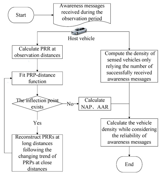
Figure 1.
Density estimation procedure of our proposed method.
3.2. System Model and Assumptions
Figure 2a illustrates connected vehicles in a highway scenario featuring several lanes in both directions. The host vehicle receives awareness messages from remote vehicles within its communication range . Since the communication range (normally hundreds of meters) is much greater than the road width, the highway can be abstracted into a one-dimensional (1D) line, as shown in Figure 2b, and the vehicles can be represented as dots on the line. The following assumptions are given.
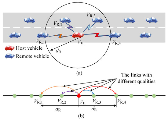
Figure 2.
Highway scenario and abstract model. (a) Highway scenario; (b) Abstract model.
- (a)
- Vehicles are distributed homogeneously on the highway, with a real vehicle density ;
- (b)
- All vehicles are equipped with the same on-board wireless transmission devices, which means the technology penetration rate is 100%;
- (c)
- All devices on the vehicles have the same configurations, including transmit power , data rate , and so on;
- (d)
- The received power with distance d away from the transmitter follows a fading/shadowing channel model, which can be expressed as follows [23]:where is the path loss. is a random gain variable representing the effects of fading and shadowing, characterized by the probability density function (PDF) of the power : .
- (e)
- A deterministic communication range is assumed, where [23], and is the receiving power threshold. According to the path loss law, we havewhere is the reference distance, is the path loss exponent, and is a dimensionless constant in the path loss law determined by the carrier frequency f and the reference distance for the antenna far field, and c is the speed of light.
The key assumption (a) is the homogeneous distribution of vehicles, which can be used to eliminate the density parameter in Equation (12). However, in reality, vehicles are rarely distributed homogeneously. In this case, even if the average vehicle density on a road segment is applied, the proposed model may experience a reduction in accuracy on a local road segment. This issue might be mitigated by splitting the road segment into smaller sub-segments and assuming a homogeneous distribution within each sub-segment. Nevertheless, there are still several unresolved issues, such as determining the optimal method for splitting the road segment.
Another noteworthy point is that, in order to improve the simulation speed of network-level communication, the PHY layer is usually abstracted into several simple factors, such as the channel model and the signal-to-interference-plus-noise ratio (SINR) threshold, which are combined to determine whether a packet can be successfully received. In this paper, although the channel model and the SINR threshold are assumed in the simulations, the proposed density estimation method is not based on these assumptions. Thus, the proposed method does not show sensitivity to the assumptions regarding the channel model and the SINR threshold. However, the statistical range in the method is limited by the communication range. We employ the path loss model to estimate the communication range, as shown in Equation (2), which is typically suitable for highway scenarios. In practice, an appropriate model can be selected based on the scenario to set a reasonable communication range, or the communication range can be adaptively adjusted according to the scenario.
4. Broadcast Reliability and Vehicle Density Estimation
The density of the sensed vehicles can be estimated based solely on the received awareness messages. In this section, the broadcast reliability metric AAR is introduced, defined as the ratio of the number of sensed vehicles to the total number of vehicles. Incorporating this metric allows the vehicle density estimate to be further refined with improved accuracy.
4.1. Packet Reception Ratio (PRR) Estimation
PRP is a link-level reliability metric defined as the probability that a packet from the transmitter is received successfully by the receiver . In contrast, PRR refers to the ratio of the number of packets successfully received by to the total number of packets transmitted by . PRR is a statistical metric and serves as an empirical estimate of PRP, reflecting its observed value through measurements or simulations:
where is the total number of packets transmitted by the remote vehicles, and is the number of packets received successfully by the host vehicle.
In reality, the PRR values are measured by the host vehicle as statistical samples used to estimate the underlying PRP curve, which remains obscured because the lost messages caused by channel impairments are unobservable.
4.1.1. Pairwise PRR
The pairwise refers specifically to the case where the remote vehicle acts as the transmitter and the host vehicle as the receiver. According to the definition of PRR, the host vehicle can locally compute based on the awareness messages received from , as follows:
where denotes the expected number of packets broadcast by the remote vehicle during the host vehicle’s observation period , and is the number of packets successfully received out of the total packets transmitted.
If the awareness messages are transmitted periodically, can be estimated by:
where is the message rate. It should be noted that even if the message rate is not constant, the host vehicle can also estimate by tracking the sequence numbers of the awareness messages [42].
4.1.2. Observation Distances
Taking the host vehicle as the reference point, the highway is divided into multiple segments, and the distance from the center of each segment to the host vehicle is referred to as the observation distance. The j-th observation distance is given by
where is the total number of segments in front of or behind the host vehicle, is the segment distance increment, and is the communication range.
4.1.3. PRR Estimation over Observation Distances
The distance between the host vehicle and the remote vehicle is denoted as the receiving distance . The host vehicle can compute based on the location information included in the received awareness messages. The average PRR at the j-th observation distance can be calculated as:
where k is the number of vehicles located within the road segment .
4.1.4. PRP–Distance Function Fitting
After each observation period , the host vehicle can calculate a set of average PRRs at different observation distances. The number of calculated PRRs is denoted by m, which typically does not exceed the total number of segments (), since some road segments may not contain remote vehicles under normal conditions.
To fit the m discrete PRR–distance points into a continuous PRP–distance curve, the Savitzky–Golay (SG) filter [43] is used for smoothing and denoising, followed by a polynomial fitting process (as shown in lines 1∼7 of Algorithm 1). Meanwhile, the effectiveness of the fitting is quantified by the sum of squared errors (SSE):
where is the fitted PRP–distance function.
Ideally, the PRP–distance function is monotonically decreasing. However, under poor channel conditions, the calculated average PRRs may exhibit non-monotonic behavior with respect to distance. This is because, for some vehicles, all of their awareness messages are lost, making them unsensed. As a result, the denominator (that is, the number of packets expected by the host vehicle) in Equation (7) is smaller than the actual number, while the numerator remains the same as the actual situation, thus overestimating PRR.
The function is refitted if an inflection point is detected based on the slope. Since PRRs should decrease with receiving distances, the corresponding point is the inflection point when the slope starts to change from negative to positive. Before refitting the , some PRR–distance points must be reconstructed first, as described in the following steps (also see lines 8∼14 in Algorithm 1).
- (a)
- Among the m discrete PRR–distance points, the index of the inflection point is denoted by .
- (b)
- The index of a specific point is marked as if the NAPs derived from the subsequent points no longer meet the quality of service (QoS) requirement, which is a threshold (e.g., 99.9%).
- (c)
- Another PRR–distance point is marked as by Equation (9)where is the index of the last PRR–distance point.
- (d)
- The PRRs of the points with indices greater than are reconstructed using Equation (10):where s is the slope calculated from two PRR–distance points with indices and , and are the PRR and distance of the point .
Finally, the PRP–distance function is refitted using the reconstructed PRRs (line 14 of Algorithm 1).
| Algorithm 1 PRPFunctionFitting(). |
| Require: discrete PRR–distance points calculated within , predefined threshold and QoS requirement . |
| Ensure: is a monotonically decreasing function |
| 1: Smoothed PRR–distance points ← linear smoothing filter (PRR–distance points) |
| 2: Initialize . |
| 3: while do |
| 4: ← polynomial fitting (Smoothed PRR–distance) |
| 5: ← calculate PRP at the observation distance according to |
| 6: calculate the sum of squared residuals by Equation (8). |
| 7: end while |
| 8: if the inflection point exists in then |
| 9: the index of the inflection point |
| 10: the index of the last point that the NAP could meet the required threshold |
| 11: the index of the point following the Equation (9) |
| 12: Calculate the slope between the points indexed and . |
| 13: Reconstruct the whose index |
| 14: redo lines to refit the |
| 15: end if |
| 16: return |
4.2. Node Awareness Probability (NAP) Estimation
NAP refers to the probability that a remote vehicle can be sensed by the host vehicle, which is defined as one minus the probability that all packets from the remote vehicle are lost by the host vehicle within the given observation period [44]. NAP can be calculated as follows:
where is the message rate, d is the distance between the transmitter and receiver, is the observation period, and stands for the binomial coefficient.
4.3. Average Awareness Ratio (AAR) Estimation
AAR is defined as the proportion of the sensed vehicles to the total number of remote vehicles within a given distance d from the host vehicle. AAR can be computed as follows:
where is the observation period, and is the vehicle density. With the first assumption that vehicles are distributed homogeneously, the real vehicle density can be considered constant, and Equation (12) can be rewritten as:
4.4. Density Estimation
Based solely on the received AMs, the host vehicle can estimate the vehicle density using the following expression:
where denotes the number of sensed vehicles within the communication range of the host vehicle. To enhance this estimate, the metric AAR can be incorporated, yielding a refined vehicle density:
5. Simulations
We conducted a series of simulations to evaluate the proposed density estimation method. In these simulations, SUMO [45] was used for traffic simulation, while NS2 was employed for network simulation. Traffic snapshots at varying densities were captured to validate the effectiveness of the proposed approach. The following sections provide a detailed description of the simulation setup and results.
5.1. Simulation Settings
5.1.1. Traffic Scenario
We adopt the traffic simulation software SUMO to generate mobility traffic on a two-lane, two-way highway road. Each lane is 5 km long and 3.2 m wide. A total of 14 traffic scenarios are created by varying the number of vehicles on the road from 100 to 1400, in increments of 100.
5.1.2. Communication Settings
NS2 is used to simulate V2X based on IEEE 802.11p in the highway scenario. The Nakagami channel fading model is employed to characterize the wireless channel conditions [23]. The observation period is set as , as recommended in [46,47]. Twenty-five observation distances are set from 10 m to 490 m, with a step size of . The other communication parameters are summarized in Table 2. These parameters are configured to comply with the IEEE 802.11 protocol, with some directly specified in the protocol standards [48]. They have been commonly used in prior literature [11,44], where the carrier sensing threshold corresponds to the received power at a communication range of 500 m.
Table 2.
The communication parameters of IEEE 802.11p.
Two kinds of PRR are calculated. One is regarded as the real PRR, evaluated according to the definition of PRR, that is, by calculating the ratio of the number of successfully received awareness messages to the total number of awareness messages sent in each link and then averaging. The other is the estimated PRR over observation distances calculated by Equation (7). Based on the estimated PRRs at the host vehicle, the PRP–distance function is fitted according to Algorithm 1. NAP and AAR are further given.
5.2. Simulation Process
To facilitate independent verification of the theoretical assumptions in our vehicle density estimation model, we outline a detailed experimental procedure structured around two key modules: the simulation module and the analysis module, as illustrated in Figure 3. The simulation module integrates traffic and network simulations to generate raw data, while the analysis module processes this data to derive reliability metrics and estimate vehicle density.
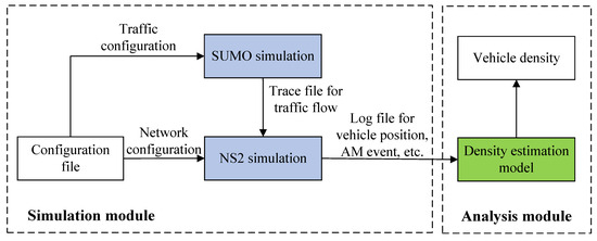
Figure 3.
Simulation process.
We initiate the process within the simulation module, utilizing SUMO for traffic modeling and NS2 for network simulation. The setup begins with defining a homogeneous highway scenario (e.g., a 5 km segment with 4 lanes) based on a traffic configuration file. Vehicle densities are configured to range from 0.02 vehs/m to 0.28 vehs/m, with an assumed 100% penetration rate of V2V devices. SUMO simulations are executed to generate trace files capturing traffic flow and mobility patterns, which are then fed into the NS2 simulation. The NS2 simulation is configured with network parameters, including IEEE 802.11p protocols, as detailed in Table 2, and it produces a log file recording vehicle positions, AM broadcast transmission events, AM broadcast reception events, and other relevant data.
In the analysis module, process the generated data to measure key reliability metrics. For each host vehicle, compute the PRR as the ratio of successfully received AMs to the total transmitted AMs from remote vehicles within an observation period, grouping values by distance bins derived from the log file. Fit a PRP–distance curve using a polynomial fitting process in Python 3.7.16 to refine deviant PRR values, ensuring alignment with theoretical trends under imperfect channel conditions. Derive the NAP for each remote vehicle as shown in Equation (11). Then, calculate the AAR by summing the NAP values over sensed remote vehicles and dividing by the estimated total vehicles, or by integrating NAP over distance for highway uniformity (as per Equation (12)).
Finally, within the analysis module, estimate vehicle density using the density estimation model. Divide the number of sensed vehicles (unique remote vehicles with at least one received AM, extracted from the log file) by the AAR to infer the total number of vehicles in range, and then compute the density. Validate the results by comparing the estimated densities against SUMO ground-truth data across varying scenarios, employing metrics such as mean absolute error (MAE) or root mean square error (RMSE) to quantify accuracy.
5.3. Simulation Results
5.3.1. PRP/NAP Estimation in Different Densities
The estimation results corresponding to the actual vehicle densities ranging from 0.02 vehs/m to 0.18 vehs/m are illustrated in Figure 4, Figure 5, Figure 6 and Figure 7. Each figure includes two subplots:
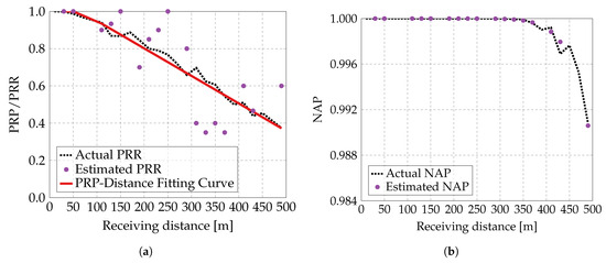
Figure 4.
Comparisons of actual and estimated reliability metrics ( vehs/m). (a) Comparison of PRRs; (b) Comparison of NAPs.
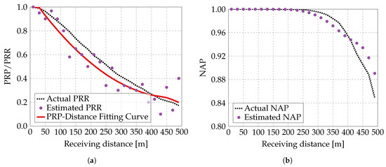
Figure 5.
Comparisons of actual and estimated reliability metrics ( vehs/m). (a) Comparison of PRRs; (b) Comparison of NAPs.
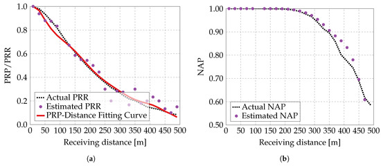
Figure 6.
Comparisons of actual and estimated reliability metrics ( vehs/m). (a) Comparison of PRRs; (b) Comparison of NAPs.
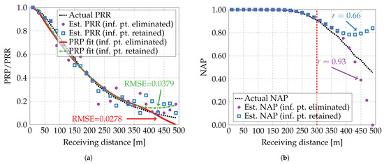
Figure 7.
Comparisons of actual and estimated reliability metrics ( vehs/m). (a) Comparison of PRRs; (b) Comparison of NAPs.
In subplot (a), the dashed line represents the real values of PRRs. The dots indicate the PRRs estimated by Equation (7) on the host vehicle. The solid line corresponds to the fitted PRP–distance curve according to the measured PRRs.
In subplot (b), the dashed line indicates the NAP calculated from the actual PRRs. The dots represent the NAP derived from the fitted PRP–distance curve.
As shown in Figure 4, Figure 5, Figure 6 and Figure 7, the actual PRR decreases with increasing receiving distance due to greater signal attenuation and a higher probability of packet loss. Additionally, for a given receiving distance, the actual PRR declines as vehicle density increases, since higher vehicle density leads to greater interference and, consequently, more severe packet loss. Furthermore, the obtained APP-layer metric, NAPs, closely matches the actual values, demonstrating the feasibility of our proposed method for estimating NAP.
5.3.2. Inflection Point Analysis
Figure 7 also shows the results from a fitted PRP–distance curve where the inflection point (abbreviated as inf. pt. in figures) is retained. The estimated values closely match the actual values for distances below 300 m; however, at longer distances, the estimates exceed the actual values. Notably, the PRP/NAP initially decreases but begins to increase beyond 400 m, indicating an inflection point in the fitted PRP–distance curve. This trend deviates from the expected monotonic decline typically observed under real conditions.
The inconsistency at longer distances arises from the fact that the host vehicle fails to receive any awareness messages from some remote vehicles. Figure 8 presents the number of sensed vehicles according to the awareness messages received within each 10 m receiving distance segment, up to the maximum transmission range . As illustrated, the host vehicle accurately estimates the number of vehicles within 400 m. However, beyond this distance, the number of sensed vehicles falls short of the actual count. This phenomenon occurs because, as the distance increases, the probability of successfully receiving a packet decreases due to higher path loss and interference, leading to more frequent packet losses. When remote vehicles are not sensed by the host vehicle, the PRR is overestimated, since the denominator in Equation (7) becomes smaller than the true number of vehicles. In general, higher vehicle density and longer distances lead to more severe packet losses caused by interference and channel fading, thereby making the estimation error more significant.
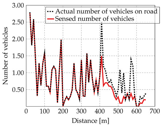
Figure 8.
The number of sensed vehicles and the real number of vehicles on the road vs. receiving distance ( vehs/m).
Therefore, when there is no inflection point in the fitted PRP–distance function, it can be used directly to compute AAR and subsequently evaluate the vehicle density. However, if an inflection point is present, the PRP–distance function must be refitted to improve accuracy. As shown in Figure 7a, the refitted PRP–distance function, with the inflection point eliminated, reduces the root mean square error (RMSE) relative to the actual PRR from 0.0379 to 0.0278. Furthermore, Figure 7b shows the Pearson correlation coefficient r of the two fitted curves relative to the actual NAP, calculated using only the points with distances greater than 300 m, which reveals a larger deviation. The correlation coefficients are and with and without eliminating the inflection point, respectively. Together with the estimated NAP, the refitted PRP exhibits a consistently decreasing trend with respect to the receiving distance, which is consistent with the expected behavior.
5.3.3. The Estimated Vehicle Density
Figure 9 compares the actual density with the two types of estimated densities of the vehicle. The results indicate that the density estimated solely from awareness messages (see star markers), as described by Equation (14), is accurate when the actual density is below 0.12 vehs/m. However, the estimation error increases noticeably as the density increases. In contrast, the density estimated by incorporating AAR (see empty square markers), as defined in Equation (15), is more accurate.
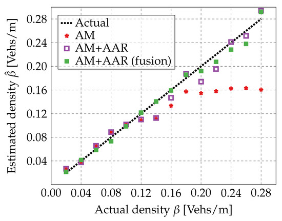
Figure 9.
Comparison between estimated and actual densities.
Furthermore, the accuracy of vehicle density estimation can be slightly improved by receiving and fusing reliability metrics estimated and shared by other vehicles via wireless communication (see the filled square markers). Specifically, each vehicle embeds its estimated reliability metric (either blindly or in response to requests from nearby vehicles) into the AM information and periodically broadcasts it to neighboring vehicles. Upon reception, a vehicle updates its reliability estimate by averaging the received metrics with its own. This collaborative approach enhances the estimation of AAR and vehicle density; however, it also introduces additional communication overhead, primarily in the form of a modest increase in AM payload size (i.e., a few extra bytes for the reliability metric), which may slightly elevate bandwidth usage and processing demands. The additional payload depends on the bytes required to represent a single reliability metric and the number of metrics transmitted per message. When each metric is stored as a string with decimal places (e.g., “0.999” for ), the size is bytes, accounting for the leading digit and decimal point. Thus, the total overhead is bytes per AM. For instance, with and , the payload increases by 125 bytes per AM.
The accuracy of the estimated density is computed as follows:
where represents the actual vehicle density and is the estimated density, which may refer to either or , as derived in Equation (14) and Equation (15), respectively.
Table 3 compares the accuracy of two types of estimated vehicle density. The proposed AM-AAR-based density estimation method improves the accuracy by 8%, increasing it from 84% to 92% when the actual density is 0.16 vehs/m. The accuracy improvement is even more significant at higher density, with a 37% increase, from 58% to 95%, when the actual density is 0.28 vehs/m. Simulation results demonstrate that this estimation method is feasible and does not incur additional communication overhead.
Table 3.
The comparison of the accuracy of the estimated vehicle density.
5.3.4. The Impact of Vehicle Speed on Estimation Accuracy
Table 3 also gives the vehicle speed corresponding to the vehicle density in the simulation. Their relationship can be described as the Greenshields model [44]. Furthermore, the analysis in Table 3 reveals a clear relationship between vehicle speed and estimated vehicle density accuracy, with speed decreasing from 21.7 m/s to 9.4 m/s as actual vehicle density increases from 0.16 to 0.28 vehicles per meter. The AM-based density estimation method shows a significant decline in accuracy from 0.84 to 0.58, likely due to its reduced effectiveness in high-density, low-speed scenarios where communication or spacing measurements are disrupted by congestion.
In contrast, the AM-AAR-based method maintains a higher and more stable accuracy range of 0.89 to 0.95, demonstrating greater robustness across varying densities and speeds. This suggests that the AM-AAR approach, possibly through adaptive adjustments, better handles the challenges of low-speed, high-density traffic, making it a preferable choice for accurate vehicle density estimation in such conditions.
5.3.5. Apply the Estimated Density to Adjust AM Rate
Herein, a potential application of the estimated vehicle density is illustrated. To alleviate communication congestion in high-density traffic scenarios and reduce data packet collisions, various congestion control mechanisms adjust transmission parameters based on vehicle density. In this context, we adopt the idea of the congestion control scheme defined in SAE J2945/1, in which the message rate is dynamically adjusted according to vehicle density [49].
According to the standard, the message transmission interval is set based on the estimated density as follows:
where B is the vehicle density coefficient (default: ), , and is the maximum allowed transmission interval.
Figure 10 compares the estimated AAR before and after adjusting the message rate (or the message transmission interval). The default message rate is set at . The results show that AAR improves with the adjusted message rate, and more than 90% of the vehicles can be sensed by the host vehicle when the density is 0.28 vehs/m.
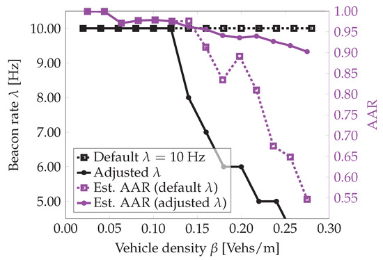
Figure 10.
Effectiveness of the message adjustment based on the proposed vehicle density estimation method.
6. Limitations and Future Developments
The model proposed in this paper is designed for homogeneous highway scenarios, relying on AM broadcasting via V2V communication. However, its application is constrained by certain limitations. To enhance its usability and generalizability, the model requires further development. Below, we summarize the key limitations and corresponding future research directions, providing actionable research plans for validation by the research community.
6.1. Limitations
- Uniform vehicle distribution assumption: The model assumes a uniform vehicle distribution (Section 3.2), which simplifies the derivation of NAP and AAR (Equations (11)–(13)) but limits its applicability to complex scenarios like intersections, where traffic patterns are non-uniform.
- Variable communication distance: The communication range (as shown in Equation (2)) varies across channel conditions, requiring specific estimation, as described in Section 3.2. This variability challenges the model’s performance in diverse environments.
- Idealized simulation environment: The validation relies on SUMO and NS2 simulations (Section 5.1) using idealized channel models (e.g., Nakagami fading), which do not account for real-world hardware constraints or environmental factors such as congestion or weather.
- High penetration rate requirement: The model assumes a high penetration rate of V2V communication devices (Section 1.1), which may not hold in scenarios with partial deployment, affecting scalability and performance.
6.2. Future Developments
To address these limitations and broaden the model’s applicability in ITS, we propose the following research directions, supported by actionable plans for independent verification:
- Extension to non-uniform scenarios: To adapt the model for intersections and urban environments, future work will incorporate non-uniform traffic patterns and multi-directional intersections in V2X broadcasts. This can be achieved by modifying NAP and AAR calculations to account for signal interference at crossings, using SUMO’s intersection modules for simulation-based validation.
- Real-world validation with hardware-in-the-loop (HIL) testing: To overcome the limitations of idealized simulations, we plan to conduct HIL experiments and field trials using real V2X devices (e.g., IEEE 802.11p or 5G NR-V2X). These experiments will measure PRR and NAP under non-ideal conditions, such as high-density congestion or adverse weather, to verify the model’s performance in real-world scenarios.
- Enhancement with advanced technologies: The newly introduced NAP and AAR metrics (Section 4) can be leveraged for theoretical studies in V2X reliability. Future work will explore integration with 5G NR-V2X or AI-enhanced estimation techniques to improve density estimation in high-density scenarios and support traffic management applications, such as maintaining density below critical thresholds.
- Optimization for partial deployment: To address the high penetration rate requirement, future research will evaluate the model’s performance under partial V2V deployment and optimize AM broadcast rates to ensure scalability and robustness in mixed traffic environments.
The proposed research directions aim to enhance the model’s utility in ITS. These developments could replace the simulation module in Figure 3 to generate raw data. The improved model, incorporating refined NAP and AAR calculations along with advanced estimation methods, would replace the analysis module to provide enhanced vehicle density estimation.
7. Conclusions
This study introduces a novel local vehicle density estimation method leveraging received AMs and the reliability metric AAR, validated through simulations. The proposed approach demonstrates several key advantages: it enables real-time density estimation, achieves high accuracy (improving by 8% and 37% at density levels of 0.16 vehs/m and 0.28 vehs/m, respectively, compared to methods relying solely on AMs), and is straightforward to implement, requiring only standard AMs without additional fields. Additionally, the method uniquely integrates reliability estimation, allowing adaptive parameter tuning to meet varying safety application requirements while optimizing energy consumption.
The simulation results highlight the method’s potential as a robust and efficient solution for traffic density estimation, distinct from existing approaches, offering a viable option for traffic management challenges. Moving forward, we plan to validate this method in real-world scenarios, including non-line-of-sight (NLOS) and intersection environments, to further refine its performance and provide actionable insights for practical deployment. Future work will also explore extensions to non-homogeneous scenarios, aiming to enhance the method’s applicability and guide the development of advanced traffic management systems.
Author Contributions
Conceptualization, Z.L.; methodology, X.W. and Z.W.; software, X.W. and Z.L.; validation, X.W. and Z.L.; formal analysis, Z.W.; investigation, Z.W.; data curation, Z.W.; writing—original draft preparation, Z.L.; writing—review and editing, X.M. and A.B.; visualization, X.W.; supervision, X.M., A.B. and J.Z.; project administration, Z.L.; funding acquisition, Z.L. All authors have read and agreed to the published version of the manuscript.
Funding
This research was funded by the Basic Scientific Research Funds of Universities of Heilongjiang Province, grant number 2023-KYYWF-1485.
Data Availability Statement
Dataset available on request from the authors.
Conflicts of Interest
Author Zhijuan Li was employed by the companies Postdoctoral Program of Heilongjiang Hengxun Technology Co., Ltd. and Shandong Hengxun Technology Co., Ltd., The remaining authors declare that the research was conducted in the absence of any commercial or financial relationships that could be construed as a potential conflict of interest .
References
- Majumdar, S.; Subhani, M.M.; Roullier, B.; Anjum, A.; Zhu, R. Congestion prediction for smart sustainable cities using IoT and machine learning approaches. Sustain. Cities Soc. 2021, 64, 102500. [Google Scholar] [CrossRef]
- Lu, J.; Li, B.; Li, H.; Al-Barakani, A. Expansion of city scale, traffic modes, traffic congestion, and air pollution. Cities 2021, 108, 102974. [Google Scholar] [CrossRef]
- Hegyi, A.; Bellemans, T.; De Schutter, B. Freeway traffic management and control. In Encyclopedia of Complexity and Systems Science; Meyers, R., Ed.; Springer: New York, NY, USA, 2009; pp. 3943–3964. [Google Scholar] [CrossRef]
- Seo, T.; Kawasaki, Y.; Kusakabe, T.; Asakura, Y. Fundamental diagram estimation by using trajectories of probe vehicles. Transp. Res. Part B Methodol. 2019, 122, 40–56. [Google Scholar] [CrossRef]
- Zheng, G.; Liu, Y.; Fu, Y.; Zhao, Y.; Zhang, Z. Perimeter control method of road traffic regions based on MFD-DDPG. Sensors 2023, 23, 7975. [Google Scholar] [CrossRef]
- Malekzadeh, M.; Papamichail, I.; Papageorgiou, M.; Bogenberger, K. Ramp metering for lane-free traffic of automated vehicles via ramp vehicle speed control. Transp. Res. Part C Emerg. Technol. 2025, 179, 105302. [Google Scholar] [CrossRef]
- Lin, Y.; Xiao, N. Identifying high-accuracy regions in traffic camera images to enhance the estimation of road traffic metrics: A quadtree-based method. Transp. Res. Rec. 2022, 2676, 522–534. [Google Scholar] [CrossRef]
- Shladover, S.E. Connected and automated vehicle systems: Introduction and overview. J. Intell. Transp. Syst. 2018, 22, 190–200. [Google Scholar] [CrossRef]
- Li, W.; Cao, D.; Tan, R.; Shi, T.; Gao, Z.; Ma, J.; Guo, G.; Hu, H.; Feng, J.; Wang, L. Intelligent Cockpit for Intelligent Connected Vehicles: Definition, Taxonomy, Technology and Evaluation. IEEE Trans. Intell. Veh. 2024, 9, 3140–3153. [Google Scholar] [CrossRef]
- Sehla, K.; Nguyen, T.M.T.; Pujolle, G.; Velloso, P.B. Resource Allocation Modes in C-V2X: From LTE-V2X to 5G-V2X. IEEE Internet Things J. 2022, 9, 8291–8314. [Google Scholar] [CrossRef]
- Zhao, J.; Wang, Y.; Lu, H.; Li, Z.; Ma, X. Interference-Based QoS and Capacity Analysis of VANETs for Safety Applications. IEEE Trans. Veh. Technol. 2021, 70, 2448–2464. [Google Scholar] [CrossRef]
- Society of Automotive Engineers (SAE). V2X Communications Message Set Dictionary, J2735_SEP2024, Revised 2024-09. 2024. Available online: https://www.sae.org/standards/content/j2735_sep2024/ (accessed on 22 September 2025).
- ETSI. Intelligent Transport Systems (ITS); Vehicular Communications; Basic Set of Applications; Part 2: Specification of Cooperative Awareness Basic Service. Technical Report EN 302 637-2 V1.4.1, European Telecommunications Standards Institute (ETSI). 2019. Available online: https://www.etsi.org/deliver/etsi_en/302600_302699/30263702/01.04.01_60/en_30263702v010401p.pdf (accessed on 22 September 2025).
- Reyes, A.; Barrado, C.; López, M.; Excelente, C. Vehicle density in VANET applications. J. Ambient. Intell. Smart Environ. 2014, 6, 469–481. [Google Scholar] [CrossRef]
- Guidoni, D.L.; Maia, G.; Souza, F.S.; Villas, L.A.; Loureiro, A.A. Vehicular traffic management based on traffic engineering for vehicular ad hoc networks. IEEE Access 2020, 8, 45167–45183. [Google Scholar] [CrossRef]
- Mathiane, M.J.; Tu, C.; Adewale, P.; Nawej, M. A vehicle density estimation traffic light control system using a two-dimensional convolution neural network. Vehicles 2023, 5, 1844–1862. [Google Scholar] [CrossRef]
- Kim, T.; Hobeika, A.G.; Jung, H. Evaluation of the performance of vehicle-to-vehicle applications in an urban network. J. Intell. Transp. Syst. 2018, 22, 218–228. [Google Scholar] [CrossRef]
- Li, W.; Song, W.; Lu, Q.; Yue, C. Reliable congestion control mechanism for safety applications in urban VANETs. Ad Hoc Netw. 2020, 98, 102033. [Google Scholar] [CrossRef]
- International Organization for Standardization (ISO). ISO/TC 204–Intelligent Transport Systems (ITS). Available online: https://www.iso.org/contents/data/committee/05/47/54706.html (accessed on 23 September 2025).
- European Telecommunications Standards Institute (ETSI). ETSI Technical Committee ITS. Available online: https://www.etsi.org/committee/its (accessed on 23 September 2025).
- 3GPP. Release 14: Summary of Rel-14 Work Items. Technical Report TR 21.914, 3rd Generation Partnership Project (3GPP). 2018. Available online: https://www.3gpp.org/ftp//Specs/archive/21_series/21.914/21914-e00.zip (accessed on 22 September 2025).
- Lusvarghi, L.; Grazia, C.A.; Klapez, M.; Casoni, M.; Merani, M.L. Awareness Messages by Vulnerable Road Users and Vehicles: Field Tests via LTE-V2X. IEEE Trans. Intell. Veh. 2023, 8, 4418–4433. [Google Scholar] [CrossRef]
- Ma, X.; Trivedi, K.S. SINR-Based Analysis of IEEE 802.11p/bd Broadcast VANETs for Safety Services. IEEE Trans. Netw. Serv. Manag. 2021, 18, 2672–2686. [Google Scholar] [CrossRef]
- Abbas, F.; Fan, P.; Khan, Z. A Novel Low-Latency V2V Resource Allocation Scheme Based on Cellular V2X Communications. IEEE Trans. Intell. Transp. Syst. 2019, 20, 2185–2197. [Google Scholar] [CrossRef]
- Clancy, J.; Mullins, D.; Deegan, B.; Horgan, J.; Ward, E.; Eising, C.; Denny, P.; Jones, E.; Glavin, M. Wireless Access for V2X Communications: Research, Challenges and Opportunities. IEEE Commun. Surv. Tutor. 2024, 26, 2082–2119. [Google Scholar] [CrossRef]
- Li, Z.; Wu, X.; Li, X.; Ma, X. Interference-Based Reliability and Capacity Analysis for IEEE 802.11 Broadcast Ad-Hoc Networks on the Highway. In Proceedings of the 11th International Conference on Vehicle Technology and Intelligent Transport Systems (VEHITS 2025), Porto, Portugal, 2–4 April 2025; pp. 520–528. [Google Scholar] [CrossRef]
- Fall, K.; Varadhan, K. The ns Manual (Formerly ns-Notes and Documentation). Technical Report. The VINT Project, UC Berkeley, LBL, USC/ISI, and Xerox PARC. 2000. Available online: https://www.isi.edu/nsnam/ns/ (accessed on 22 September 2025).
- Wang, J.; Huang, Y.; Feng, Z.; Jiang, C.; Zhang, H.; Leung, V.C.M. Reliable Traffic Density Estimation in Vehicular Network. IEEE Trans. Veh. Technol. 2018, 67, 6424–6437. [Google Scholar] [CrossRef]
- Hu, Z.; Lam, W.H.; Wong, S.; Chow, A.H.; Ma, W. Turning traffic surveillance cameras into intelligent sensors for traffic density estimation. Complex Intell. Syst. 2023, 9, 7171–7195. [Google Scholar] [CrossRef]
- Sankaranarayanan, M.; Mala, C.; Jain, S. Traffic density estimation for traffic management applications using neural networks. Int. J. Intell. Inf. Technol. 2024, 20, 1–19. [Google Scholar] [CrossRef]
- Zhang, Y.; Jia, R.S.; Yang, R.; Sun, H.M. DSNet: A vehicle density estimation network based on multi-scale sensing of vehicle density in video images. Expert Syst. Appl. 2023, 234, 121020. [Google Scholar] [CrossRef]
- Shin, C.S.; Lee, J.; Lee, H. Infrastructure-Less Vehicle Traffic Density Estimation via Distributed Packet Probing in V2V Network. IEEE Trans. Veh. Technol. 2020, 69, 10403–10418. [Google Scholar] [CrossRef]
- Zhang, J.; Mao, S.; Yang, L.; Ma, W.; Li, S.; Gao, Z. Physics-informed deep learning for traffic state estimation based on the traffic flow model and computational graph method. Inf. Fusion 2024, 101, 101971. [Google Scholar] [CrossRef]
- Florin, R.; Olariu, S. Real-Time Traffic Density Estimation: Putting on-Coming Traffic to Work. IEEE Trans. Intell. Transp. Syst. 2023, 24, 1374–1383. [Google Scholar] [CrossRef]
- Barrachina, J.; Fogue, M.; Garrido, P.; Martinez, F.J.; Cano, J.C.; Calafate, C.T.; Manzoni, P. Assessing vehicular density estimation using vehicle-to-infrastructure communications. In Proceedings of the IEEE 14th International Symposium on WoWMoM, Madrid, Spain, 4–7 June 2013; pp. 1–3. [Google Scholar] [CrossRef]
- Yao, Y.; Zhou, X.; Zhang, K. Density-Aware Rate Adaptation for Vehicle Safety Communications in the Highway Environment. IEEE Commun. Lett. 2014, 18, 1167–1170. [Google Scholar] [CrossRef]
- Chen, R.; Chen, B. Traffic State Estimation Using Basic Safety Messages Based on Kalman Filter Technique. In Proceedings of the 2024 IEEE 6th International Conference on Civil Aviation Safety and Information Technology (ICCASIT), Hangzhou, China, 23–25 October 2024; pp. 1601–1610. [Google Scholar]
- Rawat, D.B.; Yan, G.; Popescu, D.C.; Weigle, M.C.; Olariu, S. Dynamic Adaptation of Joint Transmission Power and Contention Window in VANET. In Proceedings of the 2009 IEEE 70th Vehicular Technology Conference Fall, Anchorage, AK, USA, 20–23 September 2009; pp. 1–5. [Google Scholar] [CrossRef]
- Mertens, Y.; Wellens, M.; Mahonen, P. Simulation-Based Performance Evaluation of Enhanced Broadcast Schemes for IEEE 802.11-Based Vehicular Networks. In Proceedings of the VTC Spring 2008–IEEE Vehicular Technology Conference, Singapore, 11–14 May 2008; pp. 3042–3046. [Google Scholar] [CrossRef]
- Stanica, R.; Chaput, E.; Beylot, A.L. Local density estimation for contention window adaptation in vehicular networks. In Proceedings of the 2011 IEEE 22nd International Symposium on Personal, Indoor and Mobile Radio Communications, Toronto, ON, Canada, 11–14 September 2011; pp. 730–734. [Google Scholar] [CrossRef]
- Bauza, R.; Gozalvez, J. Traffic congestion detection in large-scale scenarios using vehicle-to-vehicle communications. J. Netw. Comput. Appl. 2013, 36, 1295–1307. [Google Scholar] [CrossRef]
- Society of Automotive Engineers (SAE). On-Board System Requirements for V2V Safety Communications. Technical Report SAE J2945/1_202004. 2020. Available online: https://www.sae.org/standards/content/j2945/1_202004/ (accessed on 22 September 2025).
- Cai, L.; Xu, G.; Niyato, D. ASG: An Adaptive Savitzky-Golay Method for Channel Estimation in Deep-Space Communications. IEEE Trans. Aerosp. Electron. Syst. 2025, (Early Access). 1–12. [Google Scholar] [CrossRef]
- Li, Z.; Wang, Y.; Zhao, J. Reliability Evaluation of IEEE 802.11p Broadcast Ad Hoc Networks on the Highway. IEEE Trans. Veh. Technol. 2022, 71, 7428–7444. [Google Scholar] [CrossRef]
- Krajzewicz, D.; Erdmann, J.; Behrisch, M.; Bieker, L. Recent development and applications of SUMO-Simulation of Urban Mobility. Int. J. Adv. Syst. Meas. 2012, 5, 128–138. [Google Scholar]
- Torrent-Moreno, M.; Mittag, J.; Santi, P.; Hartenstein, H. Vehicle-to-Vehicle Communication: Fair Transmit Power Control for Safety-Critical Information. IEEE Trans. Veh. Technol. 2009, 58, 3684–3703. [Google Scholar] [CrossRef]
- Papadimitratos, P.; La Fortelle, A.D.; Evenssen, K.; Brignolo, R.; Cosenza, S. Vehicular communication systems: Enabling technologies, applications, and future outlook on intelligent transportation. IEEE Commun. Mag. 2009, 47, 84–95. [Google Scholar] [CrossRef]
- IEEE Std 802.11-2020 (Revision of IEEE Std 802.11-2016); IEEE Standard for Information Technology–Telecommunications and Information Exchange Between Systems Local and Metropolitan Area Networks–Specific Requirements Part 11: Wireless LAN Medium Access Control (MAC) and Physical Layer (PHY) Specifications. IEEE: Piscataway, NJ, USA, 2021; pp. 1–4379. [CrossRef]
- Shimizu, T.; Cheng, B.; Lu, H.; Kenney, J. Comparative Analysis of DSRC and LTE-V2X PC5 Mode 4 with SAE Congestion Control. In Proceedings of the 2020 IEEE Vehicular Networking Conference (VNC), New York, NY, USA, 16–18 December 2020; pp. 1–8. [Google Scholar] [CrossRef]


Disclaimer/Publisher’s Note: The statements, opinions and data contained in all publications are solely those of the individual author(s) and contributor(s) and not of MDPI and/or the editor(s). MDPI and/or the editor(s) disclaim responsibility for any injury to people or property resulting from any ideas, methods, instructions or products referred to in the content. |
© 2025 by the authors. Licensee MDPI, Basel, Switzerland. This article is an open access article distributed under the terms and conditions of the Creative Commons Attribution (CC BY) license (https://creativecommons.org/licenses/by/4.0/).