A Performance Comparison and Enhancement of Animal Species Detection in Images with Various R-CNN Models

Abstract

Object detection is one of the vital and challenging tasks of computer vision. It supports a wide range of applications in real life, such as surveillance, shipping, and medical diagnostics. Object detection techniques aim to detect objects of certain target classes in a given image and assign each object to a corresponding class label. These techniques proceed differently in network architecture, training strategy and optimization function. In this paper, we focus on animal species detection as an initial step to mitigate the negative impacts of wildlife–human and wildlife–vehicle encounters in remote wilderness regions and on highways. Our goal is to provide a summary of object detection techniques based on R-CNN models, and to enhance the performance of detecting animal species in accuracy and speed, by using four different R-CNN models and a deformable convolutional neural network. Each model is applied on three wildlife datasets, results are compared and analyzed by using four evaluation metrics. Based on the evaluation, an animal species detection system is proposed.

1. Introduction

Object detection has been widely studied to identify objects within an image to a predefined set of object classes (object identification) and where these objects are in the image (object localization) using bounding boxes [1]. It is a basic step for computer vision and image understanding. In recent years, most of the object detectors use Deep Learning Neural Networks (DNNs) including Convolutional Neural Networks (CNNs) architectures. CNNs have several blocks of multi convolution and pooling layers to extract features such as edges, textures, and shapes, etc., and to identify and locate objects in an image [2,3,4,5,6].

An object detection framework using a Region-based CNN (R-CNN) model can be divided into four stages: (i) region of interest (RoI) selection, also known as region proposals; (ii) features extraction for each region proposal using CNN; (iii) region classification (which objects are in each proposal); and (iv) object localization by combining overlapped region proposals into a single bounding box around each detected object using bounding box regression [7,8,9,10,11]. All these processes are time consuming, thus making R-CNN slow. Several models have been proposed to improve R-CNN, including Fast R-CNN [10], Faster R-CNN [7], and Mask R-CNN [11], to speed up object detection.

The most important step in the object detection task is the extraction of significant features, in order to identify and localize objects in the image with high accuracy. However, CNN is unable to deal with the geometric deformation of objects in images. In our study of animal species detection, Deformable CNN (D-CNN) is used to improve object features extraction under different geometric deformation conditions and thus object detection accuracy is improved, as concurred by [12,13].

In this paper, we focus on improving performance in accuracy and detection speed of animal species identification and localization. This is achieved by enhancing the extracted features through adding deformable convolutional layers to the four R-CNN models. To the best of our knowledge, there is no existing work that uses this technique in animal species detection. The effect of adding these convolutional layers to the four R-CNN detectors as we investigated by evaluating the performance of these detectors using three animal datasets. The False Negative Rate (FNR) evaluation metric is added to performance evaluation; to our knowledge, this has not been done before with animal species detection. This metric is important to determine how well a model can be used in many applications, that require minimal false negative rate, such as animal species detection in remote wilderness regions and on highways to warn hikers and drivers about the presence of dangerous animals.

The rest of the paper is organized as follows: Section 2 summarizes related work in object detection, and in particular, animal species detection. Section 3 presents an overview of the basic CNN architecture. Section 4 introduces the four R-CNN models of interest. Section 5 describes the three datasets used in our experiments. Section 6 presents the methodology of animal species detection. Section 7 compares and analyzes the results of animal species detection using various R-CNN models, in detection speed and accuracy, with and without deformable convolutional layers. Finally, Section 8 concludes the paper and discusses desirable enhancements and future works.

2. Related Work in Detection

2.1. Object Detection

The traditional neural network classifiers extract features from images by using image processing feature extraction descriptors such as Haar [14], Histogram of Oriented Gradients (HOG) [15], and Scale Invariant Feature Transform (SIFT) [16]. These neural networks could not provide high object detection accuracy, as has been shown with commonly used datasets such as ImageNet [6] and MS COCO [17]. Therefore, improvement attempts have been made to the traditional neural networks with image processing descriptors for better extraction of significant features to improve the accuracy as well as to avoid intensive computation and memory usage [8,18,19].

DNNs have a deeper structure and densely connected neural networks, such as CNNs, have become popular since the mid-2000s [20]. The characteristics which differentiate DNNs from the traditional neural networks can be summarized as [21]: (1) requiring large-scale annotated training data for learning, (2) enabling high-performance parallel computing system like GPU clusters, (3) having a sophisticated and advanced design of network structures and training strategies, and (4) using high-level characteristics of the object in feature learning strategy. Without the use of image processing feature extraction descriptors, deep CNNs can extract low (edges), mid (corners and textures), and high (parts of objects) level features as shown in Figure 1 [22]. These features can be enhanced by increasing the number of layers (depth) [23,24]. Because these neural networks are very deep, the training achieves high accuracy in complex tasks such as object detection in real-time applications. Examples of these DNNs are AlexNet [3], GoogLeNet [25], VGGNet [23], and ResNet [26].

Object detection based on DNN was introduced in Pascal Visual Object Classes (VOC) challenge in 2006 [27]. Since 2014, the ImageNet Large Scale Visual Recognition Challenge (ILSVRC) has become the main benchmark for object detection using CNNs [4,6,7]. Krizhevsky et al. [3] developed a CNN to create a bounding box around an object; however, it does not work well in images with multiple objects. Girshick et al. [9] combined region proposals with CNNs, and called their method R-CNN detector, i.e., Regions with CNN features. Due to the success of the region proposal methods, Fast R-CNN [10] was proposed to reduce the computational complexity of CNN, thus improving object detection speed and accuracy. Ren et al. [7] merged region proposal network (RPN) and Fast R-CNN into a single network called Faster R-CNN, to achieve further speed up and higher object detection accuracy. Later, Faster R-CNN was extended by predicting segmentation masks at the pixel level for each object instance with bounding box, this method is called Mask R-CNN [11]. All these improvements are significant and can be applied to animal species detection.

2.2. Animal Species Detection

There are many attempts to identify animals by assigning a label to an image; however, there are limited works in the literature that focus on animal species detection, where the location of the animal is determined as well as its identification [28,29,30,31,32,33,34,35,36,37,38,39,40,41]. Some researchers used their own datasets which contain one or only a few animal species, and others used relatively small datasets (a few thousand images only) [28,31,32]. Some researchers relied on feature extraction descriptors to classify animals [29,30]; however, several recent works have used CNNs.

Yu et al. [31] manually cropped and selected images, that only contained the entire animal body. They used a dataset which consists of over 7000 Infrared (IR) images captured by motion detection camera, called camera-trap, from two different field sites. This technique of cropping images allowed them to obtain 82% accuracy by using linear support vector machine (SVM) to classify 18 animal species. Kwan et al. [32,33] used IR videos to classify and localize objects taken from different distances, and achieved a mean average precision 89.4% by using YOLO model. Chen et al. [34] used 6-layers CNN to classify 20 animal species in their own dataset of 23,876 images with an accuracy of 38.32%. The authors used a segmentation algorithm for cropping the animals from the images and used these cropped images to train and test their system. Gomez et al. [35] used deep CNNs to identify animal species in the Snapshot Serengeti dataset. They reached 88.9% of accuracy in Top-1 (the highest probability prediction matches the actual class) and 98.1% in Top-5 (one of the five highest probability prediction matches the actual class). Willi et al. [36] identified animal species by using CNNs. They achieved an accuracy of 92.5% in Snapshot Serengeti dataset, and an accuracy of 91.4% in Snapshot Wisconsin dataset. Norouzzadeh et al. [37] used a human labeling process to train a deep active learning system to classify and count animals in to reduce images. Their system achieved an accuracy of 92.9% on cropped animal images from the Snapshot Serengeti dataset, by using ResNet-50 as a backbone network for their model. Furthermore, Norouzzadeh et al. [38] used CNN and reported an accuracy of 93.8% in classifying images that contain only a single animal in the Snapshot Serengeti dataset. The performance matched human accuracy in their experiments. However, though this work showed promising results for classifying images with only a single animal, it could not handle the challenge of localizing several animals.

Parham et al. [39] used the YOLO detector to detect zebras from a dataset of 2500 images and created bounding boxes of Plains Zebras with an accuracy of 55.6%, and Grevy’s Zebras with an accuracy of 56.6%. Zhang et al. [40] created a dataset of 23 different species in both daytime color and nighttime grayscale formats from 800 camera-traps. They compared Fast R-CNN, Faster R-CNN, and their proposed method (spatiotemporal object proposal and patch verification framework) which achieved an average F-measure score of 82.1% for animal species detection. Xu et al. [41] evaluated the Mask R-CNN model for the detection and counting of cattle (single class) from quadcopter imagery. They achieved accuracy of 94%. Gupta et al. [42] used the Mask R-CNN model with a pre-trained network ResNet-101 to detect two animal species (cows and dogs). They achieved an average precision of 79.47% in detecting cows and 81.09% in detecting dogs.

The objectives of our work are to detect multiple animals and their species in images and annotate them with bounding boxes. The three datasets used, Snapshot Serengeti, images collected by the Wildlife Program of the British Columbia Ministry of Transportation and Infrastructure (BCMOTI), and Snapshot Wisconsin, are challenging as they are all imbalanced and contain a relatively large number of animal species, thirteen in total. Furthermore, there are animal species that have similar appearance. We investigate the use of D-CNNs to enhance the detection performance.

3. Overview of CNN

CNNs have varying accuracy performance on image classification (classify what is contained in an image). The number of computation layers which have been used for features learning of input images are different depending on the visual task [23,24,25,26]. This section provides an overview of regular CNN and D-CNN.

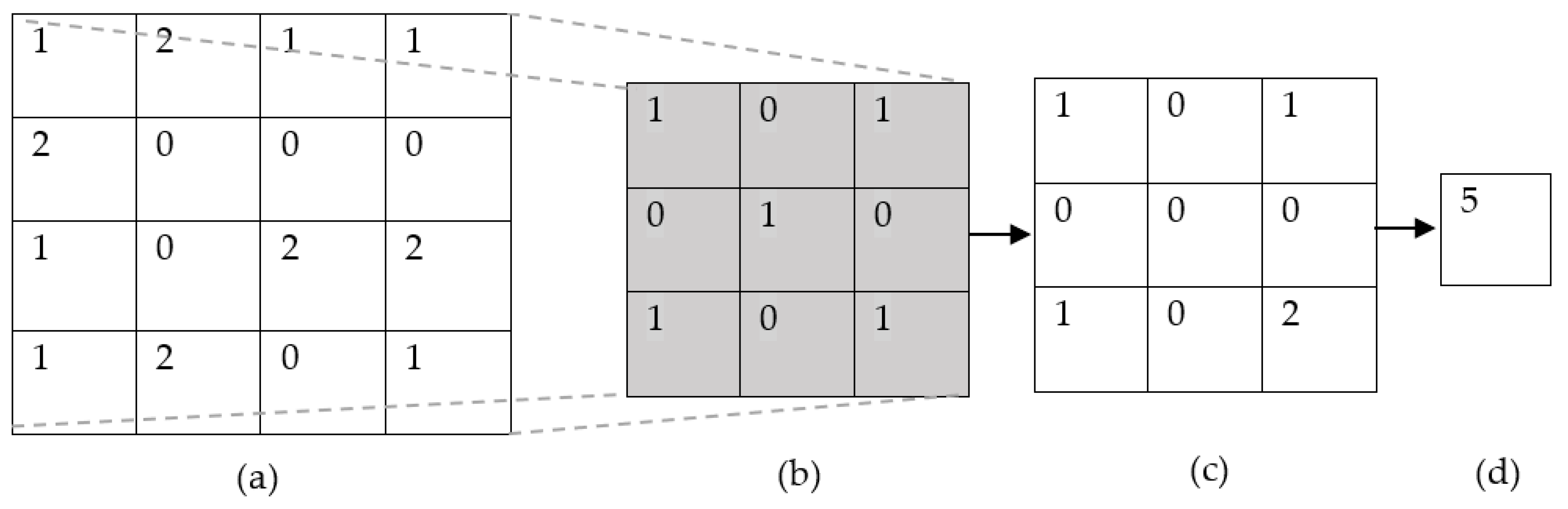
3.1. Regular CNN

Regular CNN is a deep learning algorithm which can be used to analyze input images for computer vision tasks such as image classification and object detection [4]. As shown in Figure 2, CNN has two main parts: feature learning and classification.

For feature learning, each layer in the multi-hidden layers (convolution layers plus pooling layers) perform convolution and pooling operations on its input data to produce a feature map which is a matrix representing different pixel intensities for the whole image [43,44].

As shown in Figure 3, convolution is between sliding-flipped filter window (kernel) with learned weights over input image and a local small region of the input that has the same size of that filter (receptive field); with a non-linear activation function Rectifier Linear Unit (ReLU) through a back propagation process to extract the objects’ features within the image, regardless of their location [43]. This procedure is repeated by applying multiple filters to produce a number of feature maps. Pooling is a down-sampling operation, applied to the output of convolution layer, to decrease the amount of redundant information, thus reducing computations and enabling the extraction of most significant features which are related to objects in the input image by using one of the pooling methods [45]. The most common pooling methods are average pooling and max pooling which calculate the average value for each region on the feature map or extract the maximum value from each region of the feature map, respectively, as shown in Figure 4. The max pooling function is better than average pooling in the object detection task where it helps in avoiding overfitting and in making pooling layer output invariant to small translations of the input [45,46]. Invariance to translation means that if the input has been translated by a small quantity, most of the pooled outputs’ values do not change [46]. The process of convolutional and pooling layers is repeated n times through multiple stacked layers of computation, and n is determined by the data and the visual task.

For classification, the Fully Connected Layers (FCLs) in Figure 2 are the output layers which flatten the outputs of the previous layers, the feature maps, to a single vector that can be used as an input for the Softmax layer. Each input is connected to all neurons, represented as circles in Figure 2, to predict the class of the object in the input image with an activation function Softmax, which converts the output values to conditional probabilities (normalized classification scores) for prediction, where each value ranges between 0 and 1 and all values sum to one [3,47]. The architecture of CNN has the capability to learn and extract object features, and to merge several tasks together, for example, object detection and segmentation.

Regular CNNs have been built on fixed and known geometric structure, so they cannot deal with any geometric variations in the object such as: pose, scale, viewpoint, and deformation parts [47], as illustrated in Figure 5. To solve this issue, CNN has been trained on datasets with sufficient variation, or on augmented data by changing the size, shape, and rotation angle of the object, to attain high detection accuracy. Although the problem has been solved, the training is very complex and therefore expensive. To enhance the capability of CNN to deal with geometric variations in object or deformations without using data-augmentation, D-CNNs was introduced [12,13].

3.2. D-CNN

The idea of D-CNN is to replace the regular sampling matrix that has fixed locations, as the 3 x 3 blue points in Figure 6a, with the deformable sampling matrix that has movable locations as the orange points in Figure 6b,c. These orange points are redistributed to other locations depending on the shape of the object with learned augmented offsets (the green arrows). The structure of the deformable sampling matrix can be obtained by a convolution algorithm that calculates the offset of the sampling position to learn the objects’ geometrical properties [12,13]. Each point in the regular sampling matrix is moved after adding the learnable offset to each of them, resulting in a deformable sampling matrix.

D-CNN consists of two parts: regular convolution layers to generate feature maps for the whole input image, and additional convolution layers (deformable convolution layers) for offsets to be learned from each feature map where they can be trained easily by using back propagation from end-to-end without any supervision. These additional convolution layers increase the detection performance of the network at the cost of adding a small amount of computations for offset learning. In Section 7.2., our experimental results show that after adding deformable convolutional layers to the four R-CNN models, the animal species detection accuracy is improved.

4. R-CNN Models

In general, the four R-CNN models consist of two stages as shown in Figure 7. The first is RoI or region proposals algorithm, that finds regions from the feature maps (output of CNN 1) that might contain objects and generates bounding box for each region. The second is the region pooling layer, where it detects and removes all the overlapped regions, as well as converts the extracted proposals to fixed size by doing max-pooling on them. The fixed size of proposals is required by FCLs in CNN 2 and the bounding box regressor to identify and localize objects [11].

This section provides an overview of R-CNN, Fast R-CNN, Faster R-CNN, and Mask R-CNN models. Each model attempts to improve accuracy and speed up processing.

4.1. R-CNN

The R-CNN architecture is divided into five stages as shown in Figure 8. It starts by using a selective search algorithm to generate hundreds to thousands of region proposals for an input image. These region proposals are cropped and resized [1,48]. Then, each resized region proposal is fed into CNN to extract object features. The output of each CNN is the input of a linear SVM to identify the regions of objects in image [49]. Finally, these identified regions are adjusted by using the linear bounding box regressor, to tighten and to refine the final bounding boxes of the detected objects [50].

Selective search algorithm generates regions based on a segmentation approach. It combines both object search and segmentation to detect all the possible locations of objects. In terms of segmentation of object and non-object, the image structures including object size, color similarities, and texture similarities, are used to obtain many small segmented areas. Then, a bottom-up approach is typically used as part of the selective search algorithm to merge all the similar areas to get more accurate and larger segmented areas to produce the final candidate region proposals [51,52].

The R-CNN model cannot be applied to real-time applications because:

• Network processing is expensive and slow due to the use of selective search algorithm, where hundreds to thousands of region proposals need to be classified for each image.
• R-CNN sometimes generates bad candidate region proposals as the selective search is a fixed algorithm which has no learning capabilities.

At the same time, the training of the R-CNN model is complex and requires a big memory space, since R-CNN has to train three different models separately: CNN, SVM, and bounding box regressor.

4.2. Fast R-CNN

The same developer of R-CNN proposed a modified model, the Faster R-CNN [10], to solve some of the R-CNN limitations. As shown in Figure 9, in Fast R-CNN, CNN is used to extract features and produce feature maps for the whole input image instead of each region proposal as in R-CNN. Thereby, Fast R-CNN can save time and memory compared to R-CNN. From the feature maps of the whole image, and RoI which are identified by the selective search algorithm, regions are cropped out to a fixed size feature map for each region proposal by using the region pooling layer. Then, these feature maps of each region are flattened to a vector by FCLs and fed to Softmax classification and bounding box regressor to predict the class and bounding box locations for each object in the image.

Despite the advantages of Fast R-CNN in reducing used memory and processing time, and increasing detection accuracy, the selective search algorithm that generates region proposals is still a bottleneck of the model processing time.

4.3. Faster R-CNN

In this improved model, the selective search algorithm in the Fast R-CNN has been replaced by RPN. As shown in Figure 10, the consumed time in generating region proposals is less in RPN compared to selective search algorithm, since RPN shares most computations with Fast R-CNN, as both networks have the same convolution layers and feature maps.

As shown in Figure 11, RPN is used to generate a set of various size anchor boxes across the image [53]. Anchor boxes are proposals with different sizes and aspect ratios which have been selected based on object size and are used as a reference in the testing process for the prediction of object class and localization. These anchor boxes will be fed to a binary classifier to determine the probability of having object or not, and a regressor to create the bounding boxes of these proposals. After that, a Non-Maximum Suppression (NMS) filter is used to remove overlapping anchor boxes, by (i) selecting the anchor box that has the highest confidence score, (ii) computing the overlap between this anchor box and other anchor boxes by calculating the intersection over union (IoU), (iii) removing anchor boxes that have higher overlap than a predefined overlap threshold, and (iv) repeating steps (ii) and (iii) until all overlapping anchor boxes are removed [54].

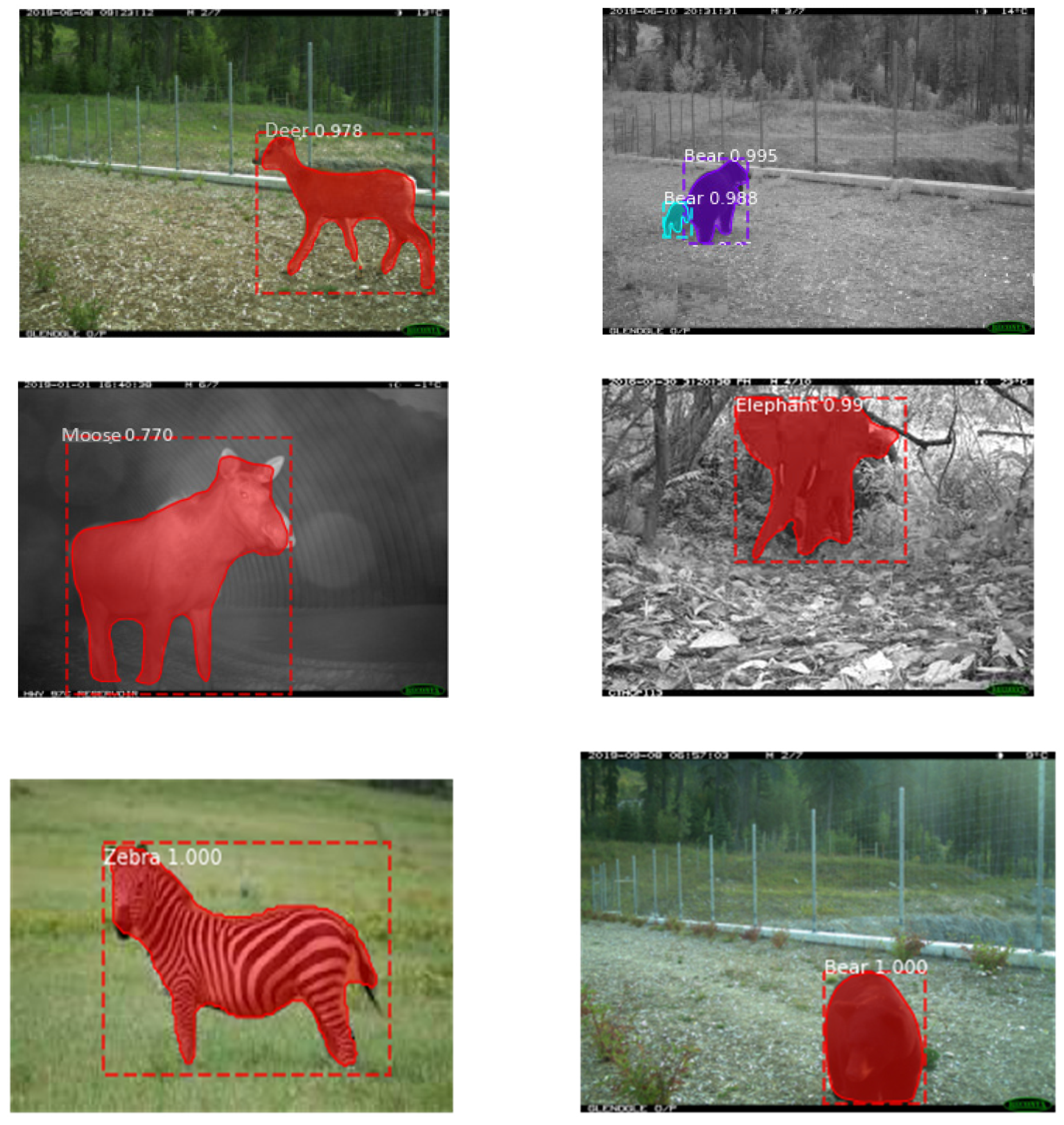
4.4. Mask R-CNN

Mask R-CNN is an extension of Faster R-CNN especially used for instance segmentation to specify which pixel is a part of which object in an image [53,55,56]. Segmentation labels each pixel in an image with an object class, and then assigns each pixel to an instance, where each instance corresponds to an object in an image. Two types of segmentations have been applied on the image in Figure 12a. Semantic segmentation, as shown in Figure 12b, does not differentiate instances of the same class (there is one bounding box for the two bears). On the other hand, instance segmentation using Mask R-CNN, as shown in Figure 12c, segments and distinguishes between objects of the same class individually in an image and localize each object instance with a bounding box (there is a bounding box for each bear).

As shown in Figure 13, Mask R-CNN consists of two parts: (i) Faster R-CNN for object detection, and (ii) Fully Convolutional Network (FCN) for providing segmentation masks on each object (object mask) [53]. In Faster R-CNN, the regions which have been resized by RoI pooling layer are slightly misaligned from the original input image. It is not important in bounding boxes; however, it has a negative effect on instance segmentation. So, Mask R-CNN uses the RoI Align layer to overcome this problem and to align more precisely by removing any quantization operations [57].

5. Animal Datasets

5.1. Datasets Used in Our Study

In our research, we used three datasets: (1) the Snapshot Serengeti dataset [58], (2) the dataset furnished by BCMOTI, and (3) the Snapshot Wisconsin dataset [59]. The Snapshot Serengeti is the dataset for the animal species in Africa (Serengeti National Park in Tanzania). A total of 712,158 images for seven species (lion, zebra, buffalo, giraffe, fox, deer, and elephant) were selected. The BCMOTI dataset has 53,000 images for eight species (bear, moose, elk, deer, cougar, mountain goat, fox, and wolf) as they are commonly seen in highways and remote areas in Canada. The Snapshot Wisconsin dataset was collected in North America by using 1037 camera-traps placed in a forest in Wisconsin. It contains 0.5 million images for different animal species, six types of animals have been chosen (bears, deer, elk, moose, wolf, and fox) since encounters between these animals and vehicles typically lead to severe crashes on highways. These animals are sometimes involved in tragic direct encounters with humans as well.

In the three datasets, the classes are imbalanced, and this is an issue to be dealt with in the future. The images were labeled by human volunteers as empty or as the name of animal species. The images in the datasets have resolutions ranging between 512 × 384 and 2048 × 1536 pixels. Snapshot Serengeti, BCMOTI, and Snapshot Wisconsin differ in many aspects such as dataset size, camera placement, camera configuration, and species coverage, thus allowing one to draw more general conclusions.

5.2. Limitations of Datasets

Detection of animal species in images is challenging due to images’ conditions. In some instances, the whole animal covers only a small area of the field of view as shown in Figure 14a. In other instances, two or more animals are too close from the field of view and combined with each other, as shown in Figure 14b. Sometimes, only part of the animal is visible in the field of view, as shown in Figure 14c,d. Furthermore, different lighting conditions, shadows, and weather, as shown in Figure 14e,f, can make the feature extraction task even harder.

6. Methodology of Animal Species Detection

The objective of this section is to find fast and accurate animal detector. Therefore, various R-CNN models are applied on the three animal datasets to evaluate and to compare their performance in terms of accuracy and speed. Moreover, D-CNN has been integrated into R-CNN models to enhance the extracted features, which in return improves the models’ capability in detecting animals.

6.1. Features Enhancement

Regular R-CNNs extract the features from the image by using a fixed size square kernel. This kernel does not cover properly all the pixels of the target object to precisely represent it. The predicted bounding box using regular R-CNN does not cover the whole animal as shown in Figure 15a. As a result, a novel technique is required to enhance the extracted features. By adding deformable convolutional layers to the regular R-CNN animal detectors, the learning of the geometric transformation of animals is possible. These layers can produce adaptive deformable kernel and offset according to the object’s scale and shape by augmenting the spatial sampling locations in convolution layers as explained earlier in Section 3.2. Therefore, the predicted bounding box using deformable R-CNN covers the whole animal as shown in Figure 15b. After experimental tries, three deformable convolutional layers are used to learn offsets, these offsets are added to the regular grid sampling locations in the regular convolution. The detection capability and accuracy are enhanced as reported later in Figures for the three datasets used.

6.2. Training

Each of the three datasets has been split into 70% for training, 15% for validation, and 15% for testing, which are the commonly used percentages in similar research. In the training of deep learning models, it is important to find the significant values of hyper-parameters such as: learning rate, batch size, number of iterations, etc. Reaching the optimum performance of a model is achieved by experiment using various values for these hyper-parameters [60]. A validation dataset is used as well to fine tune the model for overfitting and for adjusting these hyper-parameters.

The eight R-CNN models (with and without deformable convolutional layer) were trained by the back propagation and fine-tuned on the validation set to reduce overfitting by using a learning rate of 0.0025 for 32 batch size. The network of these models is initialized with the ResNet-101 [26] pre-trained model and fine-tuned end-to-end for the object detection task to enhance efficiency of training time and improve evaluation performances. All training input images were annotated by using the Image Labeler app [61] to provide labeled bounding box over the animals in these images. This box is called the ground truth box.

To identify animal species, several pre-trained models are experimented including: AlexNet, GoogleNet, VGG-16, VGG-19, ResNet-18, ResNet-50, and ResNet-101, as shown in

Table 1. Evaluation of animal species identification by using seven pre-trained models on the three datasets.

Pre-Trained Models	Accuracy of Animal Identification
AlexNet	93.1%
GoogleNet	95.9%
VGG-16	96.8%
VGG-19	96.3%
ResNet-18	96.8%
ResNet-50	97.1%
ResNet-101	97.6%

. Finally, ResNet-101 has been selected as a backbone network for the R-CNN models to detect animals in the training process. This selection of ResNet was also supported by the work of Kwan et al. [33], as they achieved good performance with YOLO using ResNet. The main reason for that selection is the ability to balance between computational complexity and the animal species detection accuracy. ResNet-101 introduces shortcut connections to speed up the convergence of the network and to avoid vanishing gradient problems during the training process, as these problems could stop the network from further training [11,26,62]. Furthermore, ResNet-101 achieves competitive accuracy and speed performance in scale-invariant feature extraction.

As shown in Figure 16, ResNet-101 consists of five regularized residual convolution blocks (Rconv.1, Rconv.2, Rconv.3, Rconv.4, and Rconv.5) with shortcut connections. These connections prevent overfitting and allow data flow from the input layer to the output layer of each block. The five blocks use 101 hidden layers to extract the image features and to produce feature maps by using 3 × 3 and 1 × 1 filter windows [26]. The output of the last block (Rconv.5) will be the input of max-pooling layer with a stride of 2 pixels to reduce the number of feature maps. FCL flattens these maps to a single vector that can be used as an input of the Softmax classification layer to deal with the thirteen classes of animal species.

Figure 17 shows the animal species detection procedure for the regular R-CNN and deformable R-CNN models. The training of the system has been applied by using the pre-trained residual network (ResNet-101). First, four regular region-based object detection models (R-CNN, Fast R-CNN, Faster R-CNN, and Mask R-CNN) are trained. Then, four new deformable region-based object detection models are trained after adding three deformable convolutional layers to the last three convolutional layers with kernel size (3 × 3) in the last block of ResN + et-101 (Rconv. 5).

Our work was carried out using MATLAB 2020b deep learning and parallel computing toolboxes and implemented on a Laptop Core i7-10750H Processor, NVIDIA GeForce RTX 2070 graphics accelerator, 32 GB RAM memory, and running a Windows 10 Professional x64 operating system.

7. Experimental Results of Animal Species Detection

7.1. Performance Evaluation Metrics

To compare and evaluate the performance of animal species detectors, four metrics are used: False Negative Rate (FNR), accuracy, mean Average Precision (mAP), and response-time.

IoU measures the overlap “intersection” between the ground truth box (actual) and the predicted bounding box divided by their union. The resulting value shows how close is the predicted bounding box to the ground truth box. To determine if the detection is positive or negative, a predefined IoU threshold value is used. It is important that the value of this threshold not to be too small or too large; in object detection researches, threshold from 0.4 to 0.7 are commonly used [6,27]. Figure 18 shows the effect of IoU threshold on the performance of Mask R-CNN. As shown in Figure 18a, the higher threshold (equal to or more than 0.5) detected two animals and produced two bounding boxes for each animal. In Figure 18b, the lower threshold (lower than 0.5) failed to detect two animals; however, it produced a bounding box for one detected animal. Thereby, FNR, accuracy, and mAP are measured using IoU threshold [17,28] at 0.5.

FNR is an essential metric in our work, where it measures the number of images that contain animals (positive) but incorrectly classified as empty images (negative). Thereby, FNR does not consider the animal class, and only measures the performance of binary classification. By defining the true positive (TP) as truly classified images with animals, and false negative (FN) as falsely classified images with animals as empty images, the FNR is calculated as:

$$\mathit{FNR}=\frac{\mathit{FN}}{\mathit{TP}+\mathit{FN}}$$

(1)

Accuracy is an evaluation metric which is calculated by dividing the total number of correctly predicted objects over the total number of input images as shown in Equation (2). TP is defined as the true detection of a ground truth box (if IoU is greater than or equal to 0.5), FN as the false detection of a ground truth box (if IoU is less than 0.5), false positive (FP) as the false detection of an object that does not exist, and true negative (TN) as the number of bounding boxes that are supposed not to be detected inside any image.

$$\mathit{Accuracy}=\frac{\mathit{TP}+\mathit{TN}}{\mathit{TP}+\mathit{FP}+\mathit{TN}+\mathit{FN}}$$

(2)

The mAP is a single number metric that combines both precision and recall by averaging precision across recall values, where it is the area under a precision–recall curve for the detections of each animal class [27,63]. Then, the result is divided by the number of classes N in the dataset as shown in Equation (3).

$$\mathit{mAP}=\frac{1}{\mathit{N}}{\Sigma }_{\mathit{i}=1}^{\mathit{N}}\mathit{A}{\mathit{P}}_{\mathit{i}}$$

(3)

where AP_i is the average precision (AP) for each animal species class (i). It is measured with the Riemann sum as the true area under the precision–recall curve [27].

Precision measures how accurate the object detection model is, as shown in Equation (4), so high precision means low false positive rate.

$$\mathit{Precision}=\frac{\mathit{TP}}{\mathit{TP}+\mathit{FP}}$$

(4)

Recall measures how many correct detections are found by the object detection model, as shown in Equation (5), so high recall means a low false negative rate.

$$\mathit{Recall}=\frac{\mathit{TP}}{\mathit{TP}+\mathit{FN}}$$

(5)

Response-time (elapsed CPU time) is an important evaluation metric which is used to measure the amount of time MATLAB takes to detect animals in a single image for an object detector model.

7.2. Comparison Results and Discussion

The results in Figure 19, Figure 20 and Figure 21 present the performance of the eight R-CNN models (four regular and four deformable) with FNR, Accuracy (Acc.), and mAP on Snapshot Serengeti, BCMOTI, and Snapshot Wisconsin datasets, respectively. Moreover, Figure 22 presents the response-time per image (sec) of the three datasets. These figures show that deformable Mask R-CNN achieves higher performance compared to other R-CNNs models. In addition, it is able to detect and to perform instance segmentation of animal species within images. In general, the results show that the added deformable convolution layers can improve the detection performance.

In Figure 19, according to the evaluation metrics (FNR, Acc., and mAP), Mask R-CNN reaches the highest performance in both regular CNNs and D-CNNs. Furthermore, deformable Mask R-CNN provides the best result with an accuracy of 98.4% and mAP of 89.2%, while incorrectly identifying 427 images with animals in the test set as empty images.

In Figure 20, the BCMOTI dataset, which is the smallest dataset used in this work, the performance of deformable Mask R-CNN decreases to 93.3% accuracy, 82.9% mAP, and FNR is increased by 1.7%, as most of the images in this dataset were taken at night with poor resolution and from the backside of the animals, as shown earlier in Figure 14.

Figure 21 shows that by using deformable Mask R-CNN, accuracy and mAP of detection are 97.6% and 87.6%, respectively, on the Snapshot Wisconsin dataset with 0.6% FNR. In the Snapshot Serengeti dataset, the system has been trained on a larger training set than BCMOTI and Snapshot Wisconsin. Thereby, it has gained up to 5.1% accuracy compared to BCMOTI, and up to 0.8% accuracy compared to Snapshot Wisconsin. This shows the importance of having a large training set with a large number of instances in each class.

As shown in Figure 22, deformable Mask R-CNN is able to detect objects in about 0.78 s per image on all three datasets. That makes deformable Mask R-CNN, though slightly slower than the regular version, suitable for use in most real-time applications.

The image results in Figure 23 show that deformable Mask R-CNN can detect and segment single and multiple animal species with a confidence score for each class. Deformable Mask R-CNN detects animal species with higher accuracy and speed in comparison to other regular and deformable R-CNN models. Therefore, not only can deformable Mask R-CNN be applied in real-time systems to detect single and multiple animal species, but it can also produce a mask over each detected animal in the image for counting the number of occluded and overlapping animal species.

In general, our results show that deformable Mask R-CNN using ResNet-101 can detect and segment animals with high accuracy exceeding the performance of the related work, as shown in

Table 2. Related work in animal species detection: a comparison.

References	Year	Dataset	Performance	Technique
Parham et al. [39]	2016	2500 images of Plain and Grevy zebras	mAP of zebra detection: 55.6% for Plain and 56.6% for Grevy	YOLOv1 detector
Norouzzadeh et al. [37]	2019	Snapshot Serengeti	Accuracy of animal species detection 92.9%	Deep active learning
Xu et al. [41]	2020	750 images of cattles	Accuracy of cattle detection: 94%	Mask R-CNN
Gupta et al. [42]	2020	MS COCO dataset [15]	AP of detection: 79.47% for cows, and 81.09% for dogs	Mask R-CNN
Saxena et al. [64]	2021	31,774 images of various animals	mAP of animal species detection: 82.11%	Faster R-CNN
Yılmaz et al. [65]	2021	1500 images of cattle	Accuracy of cattle detection: 92.85%	YOLOv4
Sato et al. [66]	2021	2000 images of donkeys and horses	Accuracy of donkeys and horses: detection: 84.87%	YOLOv4
Our work	2021	Snapshot Serengeti, BCMOTI, and Snapshot Wisconsin	Accuracy and mAP of animal species detection, respectively: 98.4% and 89.2% in Snapshot Serengeti, 93.3% and 82.9% in BCMOTI, 97.6% and 87.6% in Snapshot Wisconsin	Deformable Mask R-CNN

. This table summarizes the datasets, performance, and techniques of our research and similar related work on animal species detection. The integration of D-CNN to Mask R-CNN improves the performance of animal species detection. Our research has an improvement over these related work due to the following reasons:

• Three datasets of different characteristics have been used for training and testing.
• Deformable convolutional layers have been added to the R-CNN detectors, which have a great effect on enhancing the extracted features, which in turn improve the performance of animal species detection.

8. Conclusions and Future Work

In this paper a review on deep learning-based object detection models: R-CNN, Fast R-CNN, Faster R-CNN, and Mask R-CNN, has been provided. Then these models are evaluated on animal images from three datasets for high precision, real-time animal species detection. Next, the accuracy and speed performance of animal species detection are provided after enhancing the extracted features by using D-CNNs. The results show that deformable Mask R-CNN is the optimal choice in real-time animal species detection, and it can achieve the best performance in FNR, accuracy, and mAP, as shown in Table 2. Deformable Mask R-CNN is capable of handling geometric variations or deformations of an object, without the need for further training on datasets, thus reducing validation time and cost. Moreover, as shown in Figure 23, Deformable Mask R-CNN provides promising results for detecting animal species at a wide range of lighting, shadows, and weather condition.

In future work, we aim to detect smaller animal species which is one of the major challenges of animal species detection and to investigate improvement by reducing FNR. Furthermore, we plan to design an efficient animal detector by improving the accuracy of animal species identification and localization in high enough speed to be applied in real-time applications. To obtain higher accuracy, we need to extract more significant features, improve pre- and post- processing methods, solve the imbalance class issue, accommodate imbalance day and night images, and enhance classification confidence. For reducing the response-time and increasing the detection speed, we need to reduce the network complexity and computation time by removing some layers from the deformable Mask R-CNN architecture. Furthermore, a comparative study of one-stage and two-stage detectors would provide insights into these approaches’ speed performance.

References

- Felzenszwalb, P.F.; Girshick, R.B.; McAllester, D.; Ramanan, D. Object Detection with Discriminatively Trained Part-Based Models. IEEE Trans. Pattern Anal. Mach. Intell. 2010, 32, 1627–1645. [Google Scholar] [CrossRef] [Green Version]
- Lipton, Z.C.; Berkowitz, J.; Elkan, C. A Critical Review of Recurrent Neural Networks for Sequence Learning. arXiv 2015, arXiv:1506.00019. [Google Scholar]
- Krizhevsky, A.; Sutskever, I.; Hinton, G.E. ImageNet classification with deep convolutional neural networks. Adv. Neural Inf. Process. Syst. 2012, 25, 1097–1105. [Google Scholar] [CrossRef]
- LeCun, Y.; Bengio, Y.; Hinton, G. Deep learning. Nature 2015, 521, 436–444. [Google Scholar] [CrossRef]
- Everingham, M.; Van Gool, L.; Williams, C.K.I.; Winn, J.; Zisserman, A. The Pascal Visual Object Classes (VOC) Challenge. Int. J. Comput. Vis. 2010, 88, 303–338. [Google Scholar] [CrossRef] [Green Version]
- Russakovsky, O.; Deng, J.; Su, H.; Krause, J.; Satheesh, S.; Ma, S.; Huang, Z.; Karpathy, A.; Khosla, A.; Bernstein, M.; et al. ImageNet Large Scale Visual Recognition Challenge. Int. J. Comput. Vis. 2015, 115, 211–252. [Google Scholar] [CrossRef] [Green Version]
- Ren, S.; He, K.; Girshick, R.; Sun, J. Faster R-CNN: Towards Real-Time Object Detection with Region Proposal Networks. IEEE Trans. Pattern Anal. Mach. Intell. 2017, 39, 1137–1149. [Google Scholar] [CrossRef] [Green Version]
- Redmon, J.; Divvala, S.; Girshick, R.; Farhadi, A. You Only Look Once: Unified, Real-Time Object Detection. In Proceedings of the IEEE Conference on Computer Vision and Pattern Recognition (CVPR), Las Vegas, NV, USA, 27–30 June 2016; pp. 779–788. [Google Scholar] [CrossRef] [Green Version]
- Girshick, R.; Donahue, J.; Darrell, T.; Malik, J. Rich feature hierarchies for accurate object detection and semantic segmentation. In Proceedings of the IEEE Conference on Computer Vision and Pattern Recognition, Columbus, OH, USA, 23–28 June 2014; pp. 580–587. [Google Scholar] [CrossRef] [Green Version]
- Girshick, R. Fast R-CNN. In Proceedings of the 2015 IEEE International Conference on Computer Vision (ICCV), Santiago, Chile, 7–13 December 2015; pp. 1440–1448. [Google Scholar] [CrossRef]
- He, K.; Gkioxari, G.; Dollár, P.; Girshick, R. Mask R-CNN. In Proceedings of the IEEE International Conference on Computer Vision, Venice, Italy, 22–29 October 2017; pp. 2961–2969. [Google Scholar] [CrossRef]
- Dai, J.; Qi, H.; Xiong, Y.; Li, Y.; Zhang, G.; Hu, H.; Wei, Y. Deformable convolutional networks. In Proceedings of the 2017 IEEE International Conference on Computer Vision (ICCV), Venice, Italy, 22 October 2017; pp. 764–773. [Google Scholar]
- Zhu, X.; Hu, H.; Lin, S.; Dai, J. Deformable ConvNets V2: More Deformable, Better Results. In Proceedings of the 2019 IEEE/CVF Conference on Computer Vision and Pattern Recognition (CVPR), Long Beach, CA, USA, 16–20 June 2019; pp. 9308–9316. [Google Scholar]
- Papageorgiou, C.P.; Oren, M.; Poggio, T. A general framework for object detection. In Proceedings of the Sixth International Conference on Computer Vision, Bombay, India, 7 January 1998; pp. 555–562. [Google Scholar] [CrossRef] [Green Version]
- Dalal, N.; Triggs, B. Histograms of Oriented Gradients for Human Detection. In Proceedings of the IEEE Computer Society Conference on Computer Vision and Pattern Recognition, San Diego, CA, USA, 20–25 June 2005; Volume 1, pp. 886–893. [Google Scholar] [CrossRef] [Green Version]
- Lowe, D.G. Distinctive Image Features from Scale-Invariant Keypoints. Int. J. Comput. Vis. 2004, 60, 91–110. [Google Scholar] [CrossRef]
- Lin, T.-Y.; Maire, M.; Belongie, S.; Hays, J.; Perona, P.; Ramanan, D.; Dollár, P.; Zitnick, C.L. Microsoft COCO: Common Objects in Context. In Computer Vision—ECCV 2014; Fleet, D., Pajdla, T., Schiele, B., Tuytelaars, T., Eds.; Springer: Cham, Switzerland, 2014. [Google Scholar]
- Lin, T.Y.; Dollár, P.; Girshick, R.; He, K.; Hariharan, B.; Belongie, S. Feature pyramid networks for object detection. In Proceedings of the IEEE Conference on Computer Vision and Pattern Recognition, Honolulu, HI, USA, 21–26 July 2017; pp. 2117–2125. [Google Scholar] [CrossRef] [Green Version]
- Li, Z.; Peng, C.; Yu, G.; Zhang, X.; Deng, Y.; Sun, J. Detnet: A Backbone network for Object Detection. In Proceedings of the IEEE Conference on Computer Vision and Pattern Recognition, Salt Lake City, UT, USA, 18–22 June 2018. [Google Scholar]
- Hinton, G.E.; Salakhutdinov, R.R. Reducing the Dimensionality of Data with Neural Networks. Science 2006, 313, 504–507. [Google Scholar] [CrossRef] [PubMed] [Green Version]
- Hinton, G.E.; Srivastava, N.; Krizhevsky, A.; Sutskever, L.; Salakhutdinov, R.R. Improving neural networks by preventing co-adaptation of feature detectors. arXiv 2012, arXiv:1207.0580. [Google Scholar]
- Zeiler, M.D.; Fergus, R. Visualizing and Understanding Convolutional Networks. In European Conference on Computer Vision; Lecture Notes in Computer Science (including subseries Lecture Notes in Artificial Intelligence and Lecture Notes in Bioinformatics); Springer: Cham, Switzerland, 2014; Volume 8689 LNCS, pp. 818–833. [Google Scholar] [CrossRef] [Green Version]
- Simonyan, K.; Zisserman, A. Very deep convolutional networks for large-scale image recognition. arXiv 2014, arXiv:1409.1556. [Google Scholar]
- Sermanet, P.; Eigen, D.; Zhang, X.; Mathieu, M.; Fergus, R.; LeCun, Y. Overfeat: Integrated recognition, localization and detection using convolutional networks. In Proceedings of the 2nd International Conference on Learning Representations, ICLR 2014, Banff, AB, Canada, 14–16 April 2014. [Google Scholar]
- Szegedy, C.; Liu, W.; Jia, Y.; Sermanet, P.; Reed, S.; Anguelov, D.; Erhan, D.; Vanhoucke, V.; Rabinovich, A. Going Deeper with Convolutions. arXiv 2014, arXiv:1409.4842. [Google Scholar]
- He, K.M.; Zhang, X.Y.; Ren, S.Q.; Sun, J. Deep Residual Learning for Image Recognition. In Proceedings of the IEEE Conference on Computer Vision and Pattern Recognition (CVPR), Las Vegas, NV, USA, 27–30 June 2016; pp. 770–778. [Google Scholar] [CrossRef] [Green Version]
- Everingham, M.; Eslami, S.M.A.; Van Gool, L.; Williams, C.K.I.; Winn, J.; Zisserman, A. The Pascal Visual Object Classes Challenge: A Retrospective. Int. J. Comput. Vis. 2015, 111, 98–136. [Google Scholar] [CrossRef]
- Schneider, S.; Taylor, G.W.; Kremer, S. Deep Learning Object Detection Methods for Ecological Camera Trap Data. In Proceedings of the 2018 15th Conference on Computer and Robot Vision (CRV), Toronto, ON, Canada, 8–10 May 2018; pp. 321–328. [Google Scholar]
- Swinnen, K.; Reijniers, J.; Breno, M.; Leirs, H. A Novel Method to Reduce Time Investment When Processing Videos from Camera Trap Studies. PLoS ONE 2014, 9, e98881. [Google Scholar] [CrossRef] [Green Version]
- Figueroa, K.; Camarena-Ibarrola, A.; Garcia, J.; Villela, H.T. Fast Automatic Detection of Wildlife in Images from Trap Cameras. Hybrid Learn. 2014, 8827, 940–947. [Google Scholar]
- Yu, X.; Wang, J.; Kays, R.; Jansen, P.; Wang, T.; Huang, T. Automated identification of animal species in camera trap images. EURASIP J. Image Video Process. 2013, 2013, 52. [Google Scholar] [CrossRef] [Green Version]
- Kwan, C.; Gribben, D.; Tran, T. Multiple Human Objects Tracking and Classification Directly in Compressive Measurement Domain for Long Range Infrared Videos. In Proceedings of the 2019 IEEE 10th Annual Ubiquitous Computing, Electronics & Mobile Communication Conference (UEMCON), New York, NY, USA, 10–12 October 2019; IEEE: Piscataway, NJ, USA, 2019; pp. 0469–0475. [Google Scholar]
- Uddin, M.S.; Hoque, R.; Islam, K.A.; Kwan, C.; Gribben, D.; Li, J. Converting Optical Videos to Infrared Videos Using Attention GAN and Its Impact on Target Detection and Classification Performance. Remote Sens. 2021, 13, 3257. [Google Scholar] [CrossRef]
- Chen, G.; Han, T.X.; He, Z.; Kays, R.; Forrester, T. Deep convolutional neural network based species recognition for wild animal monitoring. In Proceedings of the 2014 IEEE International Conference on Image Processing (ICIP), Paris, France, 27–30 October 2014; pp. 858–862. [Google Scholar]
- Villa, A.G.; Salazar, A.; Vargas, F. Towards automatic wild animal monitoring: Identification of animal species in camera-trap images using very deep convolutional neural networks. Ecol. Inform. 2017, 41, 24–32. [Google Scholar] [CrossRef] [Green Version]
- Willi, M.; Pitman, R.T.; Cardoso, A.W.; Locke, C.; Swanson, A.; Boyer, A.; Veldthuis, M.; Fortson, L. Identifying animal species in camera trap images using deep learning and citizen science. Methods Ecol. Evol. 2019, 10, 80–91. [Google Scholar] [CrossRef] [Green Version]
- Norouzzadeh, M.S.; Morris, D.; Beery, S.; Joshi, N.; Jojic, N.; Clune, J. A deep active learning system for species identification and counting in camera trap images. Methods Ecol. Evol. 2021, 12, 150–161. [Google Scholar] [CrossRef]
- Norouzzadeh, M.S.; Nguyen, A.; Kosmala, M.; Swanson, A.; Palmer, M.S.; Packer, C.; Clune, J. Automatically identifying, counting, and describing wild animals in camera-trap images with deep learning. Proc. Natl. Acad. Sci. USA 2018, 115, E5716–E5725. [Google Scholar] [CrossRef] [Green Version]
- Parham, J.; Stewart, C. Detecting plains and Grevy’s Zebras in the realworld. In Proceedings of the 2016 IEEE Winter Applications of Computer Vision Workshops (WACVW), Lake Placid, NY, USA, 10 March 2016. [Google Scholar]
- Zhang, Z.; He, Z.; Cao, G.; Cao, W. Animal Detection from Highly Cluttered Natural Scenes Using Spatiotemporal Object Region Proposals and Patch Verification. IEEE Trans. Multimed. 2016, 18, 2079–2092. [Google Scholar] [CrossRef]
- Xu, B.; Wang, W.; Falzon, G.; Kwan, P.; Guo, L.; Chen, G.; Tait, A.; Schneider, D. Automated cattle counting using Mask R-CNN in quadcopter vision system. Comput. Electron. Agric. 2020, 171, 105300. [Google Scholar] [CrossRef]
- Gupta, S.; Chand, D.; Kavati, I. Computer Vision based Animal Collision Avoidance Framework for Autonomous Vehicles. Inf. Process. Manag. Uncertain. Knowl.-Based Syst. 2021, 1378, 237–248. [Google Scholar] [CrossRef]
- Oquab, M.; Bottou, L.; Laptev, I.; Sivic, J. Learning and Transferring Mid-level Image Representations Using Convolutional Neural Networks. In Proceedings of the 2014 IEEE Conference on Computer Vision and Pattern Recognition, Columbus, OH, USA, 23–28 June 2014; pp. 1717–1724. [Google Scholar] [CrossRef] [Green Version]
- Oquab, M.; Bottou, L.; Laptev, I.; Sivic, J. Weakly supervised object recognition with convolutional neural networks. HAL 2014. Available online: https://hal.inria.fr/hal-01015140v1.
- Kavukcuoglu, K.; Ranzato, M.; Fergus, R.; LeCun, Y. Learning invariant features through topographic filter maps. In Proceedings of the 2009 IEEE Conference on Computer Vision and Pattern Recognition, Miami, FL, USA, 20–25 June 2009; pp. 1605–1612. [Google Scholar]
- Goodfellow, I.; Bengio, Y.B.; Courville, A. Adaptive Computation and Machine Learning Series (Deep Learning); The MIT Press: Cambridge, MA, USA, 2016; Available online: Academia.edu (accessed on 15 August 2020).
- Bishop, C.M. Pattern Recognition, and Machine Learning; Springer: New York, NY, USA, 2006; Volume 128, pp. 1–58. Available online: Academia.edu (accessed on 15 August 2020).
- Uijlings, J.R.R.; van de Sande, K.E.A.; Gevers, T.; Smeulders, A.W.M. Selective Search for Object Recognition. Int. J. Comput. Vis. 2013, 104, 154–171. [Google Scholar] [CrossRef] [Green Version]
- Ding, S.; Zhang, X.; An, Y.; Xue, Y. Weighted linear loss multiple birth support vector machine based on information granulation for multi-class classification. Pattern Recognit. 2017, 67, 32–46. [Google Scholar] [CrossRef]
- He, Y.; Zhu, C.; Wang, J.; Savvides, M.; Zhang, X. Bounding Box Regression With Uncertainty for Accurate Object Detection. In Proceedings of the 2019 IEEE/CVF Conference on Computer Vision and Pattern Recognition (CVPR), Long Beach, CA, USA, 15–20 June 2019; Institute of Electrical and Electronics Engineers (IEEE): Piscataway, NJ, USA, 2019; pp. 2883–2892. [Google Scholar]
- Deng, J.; Dong, W.; Socher, R.; Li, L.-J.; Li, K.; Fei-Fei, L. ImageNet: A large-scale hierarchical image database. In Proceedings of the 2009 IEEE Computer Society Conference on Computer Vision and Pattern Recognition, Miami, FL, USA, 20–25 June 2009; pp. 248–255. [Google Scholar]
- Dai, J.; He, K.; Sun, J. Convolutional feature masking for joint object and stuff segmentation. In Proceedings of the 2015 IEEE Conference on Computer Vision and Pattern Recognition (CVPR), Boston, MA, USA, 7–12 June 2015; Institute of Electrical and Electronics Engineers (IEEE): Piscataway, NJ, USA, 2015; pp. 3992–4000. [Google Scholar]
- Long, J.; Shelhamer, E.; Darrell, T. Fully convolutional networks for semantic segmentation. In Proceedings of the IEEE Conference on Computer Vision and Pattern Recognition, Boston, MA, USA, 7–12 June 2015; pp. 3431–3440. [Google Scholar] [CrossRef] [Green Version]
- Prokudin, S.; Kappler, D.; Nowozin, S.; Gehler, P. Learning to Filter Object Detections. In Transactions on Computational Science XI; Springer Science and Business Media LLC: Berlin/Heidelberg, Germany, 2017; Volume 10496, pp. 52–62. [Google Scholar]
- Dai, J.; He, K.; Sun, J. Instance-Aware Semantic Segmentation via Multi-task Network Cascades. In Proceedings of the 2016 IEEE Conference on Computer Vision and Pattern Recognition (CVPR), Las Vegas, NV, USA, 27–30 June 2016; Institute of Electrical and Electronics Engineers (IEEE): Piscataway, NJ, USA, 2016; pp. 3150–3158. [Google Scholar]
- Arnab, A.; Torr, P.H.S. Pixelwise Instance Segmentation with a Dynamically Instantiated Network. In 2017 IEEE Conference on Computer Vision and Pattern Recognition (CVPR), Honolulu, HI, USA, 21–26 July 2017; Institute of Electrical and Electronics Engineers (IEEE): Piscataway, NJ, USA, 2017; pp. 879–888. [Google Scholar]
- Wu, H.; Siebert, J.P.; Xu, X. Fully Convolutional Networks for automatically generating image masks to train Mask R-CNN. arXiv 2020, arXiv:2003.01383v1. [Google Scholar]
- Labeled Information Library of Alexandria: Biology and Conservation (LILA BC). [Snapshot Serengeti]. Available online: http://lila.science/datasets/snapshot-serengeti (accessed on 27 August 2020).
- Snapshot Wisconsin, A Volunteer-Based Project for Wildlife Monitoring. [Snapshot Wisconsin]. Available online: https://dnr.wisconsin.gov/topic/research/projects/snapshot (accessed on 1 May 2020).
- Fan, Q.; Brown, L.; Smith, J. A closer look at Faster R-CNN for vehicle detection. In Proceedings of the 2016 IEEE Intelligent Vehicles Symposium (IV), Gotenburg, Sweden, 19–22 June 2016; Volume 1, pp. 124–129. [Google Scholar]
- MATLAB. Available online: https://www.mathworks.com/help/vision/ug/get-started-with-the-image-labeler.html (accessed on 15 January 2020).
- Khan, A.; Sohail, A.; Zahoora, U.; Qureshi, A.S. A survey of the recent architectures of deep convolutional neural networks. Artif. Intell. Rev. 2020, 53, 5455–5516. [Google Scholar] [CrossRef] [Green Version]
- Henderson, P.; Ferrari, V. End-to-End Training of Object Class Detectors for Mean Average Precision. In Asian Conference on Computer Vision; Springer: Cham, Switzerland, 2016; pp. 198–213. [Google Scholar] [CrossRef] [Green Version]
- Saxena, A.; Gupta, D.K.; Singh, S. An Animal Detection and Collision Avoidance System Using Deep Learning. Adv. Graph. Commun. Packag. Technol. Mater. 2021, 668, 1069–1084. [Google Scholar] [CrossRef]
- Yilmaz, A.; Uzun, G.N.; Gurbuz, M.Z.; Kivrak, O. Detection and Breed Classification of Cattle Using YOLO v4 Algorithm. In Proceedings of the 2021 International Conference on INnovations in Intelligent SysTems and Applications (INISTA), Kocaeli, Turkey, 25–27 August 2021; pp. 1–4. [Google Scholar]
- Sato, D.; Zanella, A.J.; Costa, E.X. Computational classification of animals for a highway detection system. Braz. J. Veter-Res. Anim. Sci. 2021, 58, e174951. [Google Scholar] [CrossRef]