Abstract
Interferometry Synthetic Aperture Radar (InSAR) is an advanced remote sensing technique for studying the earth’s surface topography and deformations; it is used to generate high-quality Digital Elevation Models (DEMs). DEMs are a crucial and primary input to various topographical quantification and modelling applications. The quality of input DEMs can be further improved using fusion methods, which combine multi-sensor or multi-temporal datasets intelligently to retrieve the best information from the input data. This research study is based on developing a Neural Network-based fusion approach for improving InSAR-based DEMs in plain and hilly terrain parts of India. The study areas comprise relatively plain terrain from Ghaziabad and hilly terrain of Dehradun and their surrounding regions. The training dataset consists of DEM elevations and derived topographic attributes like slope, aspect, topographic position index (TPI), terrain ruggedness index (TRI), and vector roughness measure (VRM) in different land use land cover classes of the study areas. The spaceborne altimetry ICESat-2 ATL08 photon data are used as a reference elevation. A Feed Forward Neural Network with a backpropagation algorithm is trained based on the prepared training samples. The trained model produces fused DEMs by learning the relationship between the input and target samples; this is used to predict elevations for the test areas. The accuracy of results from the models is assessed with TanDEM-X 90 m DEM. The fused DEMs show significant improvement in terms of RMSE (Root Mean Square Error) over the input DEMs with an improvement factor of 94.65% in plain areas and 82.62% in hilly areas. The study concludes that the ANN with its universal approximation property can significantly improve the fused DEM.
1. Introduction
Digital Elevation Models (DEMs) are one of the most crucial and key inputs for several topographical applications. DEM is a three-dimensional digital representation of the earth terrain showing the elevation profile or height variations. A DEM depicts the continuous earth surface by a large number of points having x, y and z information in a given coordinate system [1]; it takes the form of a raster grid or a vector triangulated irregular network (TIN) form. DEM is a primary input to various modelling and quantifying processes in multiple disciplines such as hydrology [2,3], glaciology, soil sciences, agricultural, urban, climate studies, forestry, disaster risk monitoring [4], geomorphology, and environmental monitoring [5]. The remote sensing technologies have transformed in past times and so has evolved the process of DEM generation. Different sensors provide a variety of input for producing DEMs such as stereo-pairs from optical sensors, spaceborne SAR satellites image pairs for Interferometry or radargrammetry, LiDAR point clouds and digitization of contour maps. Every technique developed for generating an elevation model has its own advantages and limitations. Due to the advantages of microwave active sensors over other conventional methods, SAR Interferometry has emerged as an advanced technique for generating high-precision DEMs [6].
The Synthetic Aperture Radar (SAR) is an active microwave sensor that provides high-spatial and good temporal resolution SAR image pairs for the Interferometry process for generating DEMs. The phase variation from the earth surface targets as recorded in the backscatter of the radar signals is transformed to elevation values in the interferometry technique using two SAR acquisitions taken for the same area with some time difference or different viewing angles. The SAR images are compared after registration and interference between them produces a fringe map termed an interferogram [7]. The elevation values derived from the interferometry by the transformation of phase variations are highly correlated with the terrain topography and deformation patterns can also be mapped from this [8,9]. The availability of a large number of spaceborne SAR sensors such as the Sentinel-1A/ 1B, RADARSAT-1/2, ALOS PALSAR- 1/2, TerraSAR-X and TanDEM-X, provides high spatial and temporal resolution images to carry out interferometry process for the generation of DEMs. A DEM being a crucial input to varied applications, can be improved by employing fusion techniques. The task of improving different forms of DEMs has been extensively researched and presented by several authors. Fusion is a technique of combining multi-source data to improve upon individual values and produce a high-quality representation of the data. The first case of data fusion in earth sciences was employed in numerical weather forecasting, which belongs to wider estimations and control theories [10]. The fusion of information from different sources is useful in obtaining a high-resolution elevation model that can be analyzed for its quality using other different types of datasets such as LiDAR data or multispectral images [11,12,13]. Various techniques have been followed for fusing the DEMs such as statistical measures of central tendencies, Sparse representation [14], Kalman filtering [15,16], and ANN framework [17]. A novel empirical model is developed for the improvement of InSAR-based DEMs using the DEM fusion approach in the plain terrain of Ghaziabad and its surrounding regions, known as Successive Best Pixel Selection Approach (SBPSA); this is based on deriving better elevation values from multiple InSAR-based DEMs based on firstly, coherence values and then select the nearest to truth elevation values in generating improved fused DEMs. The accuracy assessment for fused DEMs shows significant improvement with an RMSE of 0.98 m for fused output DEM in comparison to 1.58 m and 1.20 m RMSE of individual input DEMs [18].
TanDEM-X and Cartosat-1 elevation data are fused with support of ANN which is used as a predictive weight mapping model in a weighted averaging fusion for different land types in urban areas of Munich, Germany [17]. An attempt was made to improve SRTM DEM using a multilayer perceptron type ANN in coastal areas to obtain a global coastal DEM reducing the vertical error regression by combining information of vegetation indices and LiDAR reference data [19]. An alternative method of fusion in place of interpolation techniques is an ANN model designed in MATLAB to estimate unknown heights of a DTM [20]. The quality of SRTM DEM is improved in the dense urban city of Nice, Singapore with the usage of multispectral Sentinel-2 and Google Earth imagery as inputs and high-precision reference DEM as a target in a multi-channel CNN model using a U-Net structure. The model is implemented in the MATLAB Deep Learning toolbox and the results showed an RMSE of 4.8 m in contrast to the 9.2 m RMSE of the original DEM [21]. Recent research work has shown the improvement of Satellite DEM that is TanDEM-X (12 m DEM) using multispectral imagery and predictive learning capability of the ANN models. The ANN model is trained in the Nice area using various indices from Sentinel-2 multispectral data and ground truth information for the area and it is validated over the Singapore site. The trained model is then tested over a new test study site of Vietnam where the ground truth is not available [22].
Although, from the literature survey it can be inferred that very less research work has been done for DEM improvement using an ANN-based approach specifically for the widely diverse topography of India. Thus, the adaptive learning of Neural Networks provides scope for developing methods and models which can be used as a tool for performing DEM fusion to improve the existing or generated DEMs in the complex and diverse topography of the Indian region. A large number of applications employ DEM as a primary and key input; thus, an improvement of input DEM will add up to the potential of the generated outputs from these applications. Moreover, the use of precise ICESat-2 (Ice, Cloud and Land Elevation Satellite) spaceborne altimetry data as tested and validated for assessment of DEMs shall be explored in applications of ANN-based fusion models [23,24]. The precise elevation data from the ICESat-2 ATL08 (Land and Vegetation) height product provided with height uncertainty suffice for the reference elevation data in hilly and complex terrains where the collection of ground truth can be a time-consuming and difficult task. Wang evaluated the accuracy of ICESat-2 data in providing ground elevation data in the Alaska region, validating it with airborne LiDAR data and other factors like slope, vegetation covers and height of vegetation [25]. The accuracy of ICESat-2 data products is tested successfully by Zhang in the mountainous region using around 208 footprints with CORS (Continuously Operating Reference System) and UAV (Unmanned Aerial Vehicle) datasets [26]. The abundance of laser photon datasets covering the regions around the globe, provided by ICESat-2 mission has been employed in the accuracy assessment of open access InSAR-based DEMs in the Himalayan region [27]. SRTM 90 m DEM is assessed with the ICESat-2 data in Australia region for bare ground and in areas with tree cover and vegetation heights, concluding that in plain areas its accuracy is similar to SRTM DEM and showing the positive differences in vegetation areas for ATL08 product [28]. ICESat-2 is also used in the assessment of open access DEMs like TanDEM-X and CartoDEM and retrieval of building heights in urban areas [29,30].
This paper is organized in the following manner: The core concepts and background of the Artificial Neural Networks (ANN) are explained in Section 2. Section 3 describes the two study sites considered in this work and explains their various aspects along with the specifications of datasets processed in this study. Section 4 discusses in detail the processing steps and methodology followed for the development of the neural network DEM fusion framework for different topographies of the study sites. The important inferences and assessment results obtained from the neural network models are presented in Section 5. Further, Section 6 gives the important discussions made during the work and finally, Section 7 concludes the study.
2. Neural Network Fusion Framework
An Artificial Neural Network (ANN) is a part of a bigger Machine Learning class which acts or mimics the human brain and works similarly its design is based on biological neurons. The structure of a neural network is interconnected where the fundamental unit is called a neuron. The special characteristic of a neural network is that of universal approximation making it highly effective; this property makes a neural network an important tool for solving problems of varied domains including remote sensing and signal processing problems [31]. The concept of learning by a single neuron was originally presented in the work of McCulloch and Pitt’s neuron model in the 1940s. According to this model, a neuron has two main parts, a net function u and an activation function a. The net function is the weighted average sum of all the inputs and biases (Equation (1)) [31]. The activation function is a linear or non-linear transformation of inputs to desired outputs.
where the term is weighted inputs and θ is the bias or threshold of a neuron and a is the activation function for net function u.
A neural network is a non-parametric computational model that can learn the non-linear and highly complex relationship between variables. A simple model consists of an input layer, a hidden layer (or layers) and an output layer. The neurons of each layer work in a parallel combination transforming the input to desirable output as required in the application of models. Each layer is connected to the next layer forming a network. The basic operation of ANN follows the reception of information from the outside world through the input layer, which travels to the next connected layer (hidden layer) after a neuron gets activated. The activation of the neuron takes place once the threshold is reached by the weighted input and bias. The hidden layer transforms the input into desirable or meaningful outputs using transfer or activation functions. The input data comprises attributes or features of different samples that belong to different classes. The aim is to make a neural network to determine the correct output of new samples by learning the behaviour of the already classified samples in the training dataset. Weights are assigned randomly to each of the neurons; these are arbitrarily initialized values to the inputs based on the importance or amount of influence it has on the output. The activation functions or the transfer function are the mathematical functions which are differentiable in a definite range; it computes the sum of the product of weights and inputs added with biases to check whether a neuron should be activated or not. Some commonly used transfer functions are Linear, Sigmoid, TanH, ReLU (Rectified Linear Unit), Softmax functions and so on. The hidden and output layer neurons are equipped with these transfer functions [31].
The information propagates through the network in a forward direction that is from input to output layers through the hidden layers; this traversing of data in the network is termed Forward propagation and the network is called Feed Forward network. In a multi-layer perceptron (MLP) model that consists of a layered structure (based on McCulloch and Pitt’s neuron model), non-linear activation functions are used and the neurons of each layer are interconnected. The weight matrices of MLP neurons are determined by using the error-backpropagation training method, originally proposed by the Widrow-Hoff gradient descent procedure in the 1960s. A backpropagation algorithm estimates the error between the predicted and the target outputs and reduces the error gradient by propagating the training samples back and forth in the network. The weights are updated with the error gradient calculation. The rate of change in error to the change in error is called the error gradient; it is the direction of the steepest descent for the learning algorithm to obtain the global minima from the several available local minima [32]. According to Equation (2) [31], the updating of the weights takes place as below:
The updated weights is given as the sum of the previous weight with the sum of three terms: the second term describes the gradient of the mean square error with respect to that is the summation of the product of delta error and the output z corresponds to the kth training sample of jth neuron of the (L − 1)th layer; η represents the learning rate or step size; L denotes the layer. The third term is the momentum term for the adaptive adjustment of step size or learning rate with the gradient vector represented by . Momentum constant μ will be gained when the gradient vector is indicating in the same direction in each successive epoch, while a zigzag search pattern shows that the momentum term helps in minimizing the mean-square error regulating the effective gradient direction. The learning rate and the momentum are selected in the range of 0 to 1. Generally, the learning rate is kept smaller between 0 to 0.3 and momentum assumes larger values between 0.6 to 0.9. The last term represents small random noise that helps the backpropagation algorithm to leap out of the local minima during the search for global optimum minima when the magnitude of the corresponding gradient vector or momentum has diminished [31].
Generally, a Feed-Forward Multilayer Neural Network is useful for classification, regression, pattern recognition and prediction problems. A neuron of a layer is connected to the next successive layer neuron and each connection possesses a weight. The number of units in an input layer is exactly the number of input data applied to the network. A heuristic approach is applicable for obtaining an optimal architecture of the model by determining the required number of hidden layers, number of units in hidden layers, model parameters like the activation function, optimizer, number of layers, batch size, epochs and so on [33,34]; these are known as the hyperparameters, which are either selected heuristically or by hyperparameter tuning running several iterations to check the model performance. The output layer neurons are the number of classes or desired number of outputs. An ANN model can be implemented on several platforms like on TensorFlow using Keras library or with built-in applications of commercial software MATLAB NN-Toolbox (Neural Network). This study has employed both methods for designing ANN models in the study areas. MATLAB NN-Toolbox provides faster converging backpropagation algorithms other than the standard gradient descent backpropagation (traingd, traingdm). The other classes include algorithms with variable learning rates (traingda, traingdx), resilient backpropagation (trainrp), algorithms that use numerical optimization techniques like conjugate gradient (traincgf, traincgb, traincgp, trainscg), Quasi-Newton (trainbgf) and Levenberg Marquardt (trainlm) algorithms. Among the mentioned algorithms, the Levenberg Marquardt is most widely used as it converges faster by minimising the error gradient [35].
The models are designed by selecting appropriate parameters and are introduced with the training and testing datasets. The training samples include input features from different thematic layers, and the target set includes accurate reference values. The testing dataset is the one with new samples from the study areas to test the performance of the trained model. The focus of this study is to develop a method for producing a high-quality DEM which in turn caters to wide remote sensing applications like topographic mapping, hydrological modelling, glacial studies, disaster risk monitoring, climate studies, surface deformations, and so on. Thus, there is a requirement for a method or process that produces high-quality DEMs and their analysis for accuracy in diverse terrains and geographical regions.
3. Study Areas and Dataset Used
The study areas for implementing the process of fusion using a neural network-based approach are selected from diverse terrain in Indian states. The first study area is from Ghaziabad and the surrounding regions which is mainly a plain terrain region. The second study area is the hilly and undulating terrain of Dehradun and surrounding regions (Figure 1).
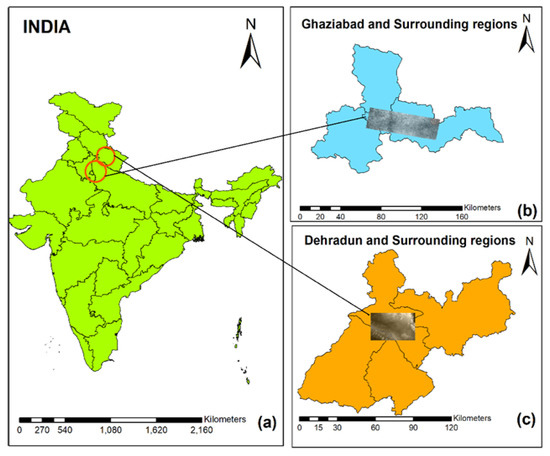
Figure 1.
Study Area Map with overlay of DEMs to show the extent of study areas: (a) India; (b) Study Area 1: Ghaziabad and Surrounding regions; (c) Study Area 2: Dehradun and Surrounding regions.
3.1. Study Area 1: Ghaziabad and Surrounding Region
This study site lies on the western edge of Uttar Pradesh state of India belonging to the Delhi-NCR (National Capital Region); it’s one of the oldest and largest cities in the state, in the vicinity of the national capital Delhi. The geographical extent of the study site is from 77° to 78° E Latitude and 28° to 29° N Longitude covering from Loni to Pilakhuwa with around 777.9 Sq Km area. The major water body is the river Hindon which segments the Ghaziabad region into Cis-Hindon on the east and Trans-Hindon on the west; it falls in the Upper-Gangetic plains having an average elevation of 214 Km. The terrain is majorly plain with elevation values varying from 60 m in eastern parts to 300 m in Northwest parts. The terrain relief is featureless having fertile land varying from alluvium soil to sandy and clayey loamy soil across the city. The climate is tropical monsoon type having warm weather round the year. The different landform types in this region include highly-dense built-ups including rural and urban settlements. The urban class includes flats, two-storey and multi-storey apartments as this region caters to large industrial sites. Other land use land cover classes are agricultural fields, croplands, barren land, roads and highways, and river; this is selected to implement and analyse the improvement of InSAR-based DEMs in a plain and largest urban area of the Indian region.
3.2. Study Area 2: Dehradun and Surrounding Region
It is the largest and most populated, capital city of Uttarakhand state; it’s located in the foothills of the Himalayas and Shivalik range in Doon Valley. The geographical area of this study site is around 3088 Sq Km. The Latitudinal and Longitudinal extent of this area is from 77°34′ to 78°18′ E and 29°58′ to 31°2′ N. The two main rivers flowing through this region are Ganga in the east and Yamuna in the west. Two major parts of this area are first, Dehradun city bounded by the Himalayas and the Shivalik ranges from north to south respectively and the second part is the Jaunsar Bawar located at the base of mountains. The geography of this area comprises highlands and hills with cooler temperatures and vast-dense forest cover. Topographically, there are two tracts, first is the Montane tract covering the entire Chakrata tehsil having high mountains, continuous steep slopes and gorges in the Jaunsar Bawar region. The sub-mountain tract is the second tract including Doon valley bounded by the Shivalik in the south and the Himalayas in the north. The hilly terrain of this region has elevation values in the ranges of 410 m in Clement town to 700 m in the Malsi area, and up to 1870–2017 m at Mussoorie. The land use land cover classes of this area comprise largely dense forest covers in Terai and Bhabar as well as the Shivalik hills with large tree canopies in Mussoorie. The Doon Valley, on the contrary, has huge settlements, including the city areas of Dehradun, Doiwala, Harrawala, Herbetpur, Rishikesh, Raiwala and Clement town area. The geomorphological and meteorological conditions of Dehradun and its surrounding regions make it highly vulnerable to natural hazards which are prone to floods, landslides, earthquakes and so on; this is an important study site for which good quality DEMs should be developed to be applied in major disaster risk management and climate study applications.
3.3. Dataset Used
Multiple DEMs using the SAR Interferometry technique are generated from Sentinel-1A and 1B image pairs for the two study regions. High-resolution multispectral data to prepare the LULC maps are obtained from the Sentinel-2 MSI product. The precise spaceborne altimetry ICESat-2 photon data are used as a reference elevation for the training of the different neural network models. Finally, the results from the ANN models are assessed for accuracy and quality in comparison to TanDEM-X 90 m DEM for the two different topographies under study. The Survey of India (SOI) Toposheets are also referred for each region to check for the range of elevation values while preparation of training and testing datasets for each of the study areas. The details and specifications of all the datasets are given in Table 1.

Table 1.
Materials used and their specifications.
4. Methodology
The steps followed to carry out the study are depicted below in Figure 2. The first step is to generate multiple InSAR-based DEMs for each of the study sites. The SAR image pairs to perform interferometry is selected mainly based on perpendicular and temporal baselines using the ASF (Alaska Satellite Facility) Vertex Data Search and Baseline tools. Other factors that affect the quality of InSAR DEMs are operating wavelength, viewing angle, Image Coherence and suitable atmospheric conditions [6,36]. Using the multi-pass interferometry from the spaceborne SAR sensors, multiple image pairs are selected in both regions. Selecting the suitable sub-swath and polarization, the two images in each pair (referred to as reference/master and secondary/slave image) are co-registered to create a stack that aligns both the products at sub-pixel accuracy to exploit the phase difference of the acquisitions. The orbit file information which is available with the image pairs containing the sensor’s positional information at the time of imaging is applied to the images. An Interferogram is generated from the stack containing the intensity image, phase image and coherence image. The phase information of DEMs is extracted by subtracting the flat-earth phase and removing the interference from the atmospheric conditions and noises from the total phase. Phase filtering is performed to further unwrap the interferogram phase properly. The most important step of phase unwrapping over the filtered subset is performed using SNAPHU (Statistical Cost, Network-Flow Algorithm for Phase Unwrapping) algorithm in the open-source SNAP software. The phase unwrapping is used for the removal of any ambiguity in the phase information of the SAR images; this unwrapped phase so obtained is transformed to elevation and the coherence band is added to the final product to obtain the DEM output. Similarly, other SAR pairs are used to produce multiple DEMs through the interferometric process for the two study areas, having varying quality depending on the particular baselines and coherence that an image pair possess.
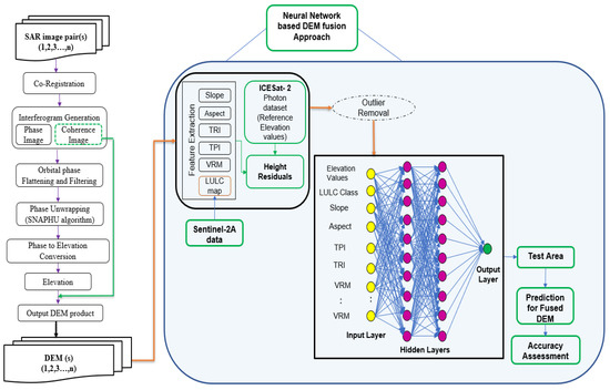
Figure 2.
Workflow of the Neural Network-based Fusion Framework for DEM Improvement.
The elevation values from these multiple InSAR-based DEMs are input to the Neural Network models. Other geometrical features or topographic attributes are generated from the DEMs to provide a deep insight into terrain information to the model. Several studies show the relationship of these attributes with the quality of DEMs [12,37]. The topographical attributes computed in this study include the Slope (the first-order derivative of the DEM or the rate of change of elevation in the up or down steepest direction of DEM), Aspect (the first-order derivative of DEM that is a measure of the steepest slope in the downhill direction), Topographic Ruggedness Index (TRI) (that is the standard deviation of slope or elevation; the difference between the elevation of a cell and the mean elevations of eight neighboring pixels [38], Topographic Position Index (TPI) (is the difference between the pixel height with the average height of the neighboring pixel [39,40], Vector Ruggedness Measurement (VRM) (is the three-dimensional perspective of the raster grid in relation to its neighbours [41] and the Land Use Land Cover classes map for both the study areas. The input data thus includes elevation values from the InSAR DEMs, DEM derivative values and the LULC class information that appears on respective nodes of the input layer. The height residuals are calculated for each of the DEMs with the precise ICESat-2 ATL08 elevation data considering the available uncertainties with the product. Further, the extracted information from the raster layers is filtered using the height residual values that fall within the range of the second standard deviation (2σ) of the mean to remove the outliers. The prepared filtered datasets are used as the training samples for the neural network models.
The suitable neural network models are designed using a Keras-based ANN model in Google Colaboratory and the MATLAB NN- Toolbox. The Keras-based models are sequential dense layer Feed-Forward Multilayer perceptron models using the backpropagation algorithm; these models are designed by selecting the appropriate number of layers, the number of neurons in each layer, activation functions used in each layer, optimizer, batch size and epochs after performing hyperparameter optimization. The training dataset includes the input DEM elevation values along with the related DEM derivative values and the reference is provided from the ICESat-2 photon points. The random state in the train-test split function is to ensure the reproducibility of the results. The model training is validated to check and prevent overtraining or undertraining by visualizing the chosen loss parameter as Mean Absolute Error (MAE). The training and validation loss curves are used to visualize the performance of the model while training with the use of different activation functions in several iterations. The best fit model architecture is selected for performing DEM fusion; this best-trained model is then tested for making predictions over new data samples of the study area which were not included in the training. The network models the relationship by combining the information from the given input and the reference (ICESat-2 elevation values). The error gradient between the predicted and the output values are minimized by the backpropagation algorithms. The model predictions are then assessed with TanDEM-X 90 m DEM to estimate the RMSE (Root Mean Square Error) as a measure of accuracy and quality of DEM. The mathematical expression of RMSE is given in Equation (3); it is a measure of the square root of the mean squared height errors between the predicted and the observed values [42].
Here, the Hi(input) refers to the ith elevation of input DEM and the Hi(Ref) is the corresponding reference elevation value which is from the ICESat-2 photon data and n denotes the total number of observations.
Another estimate of accuracy can be determined from the percentage improvement factor (%IF) which is calculated by simply taking the percentage of the difference between the RMSE of input and predicted or fused DEM RMSE over the input DEMs [43,44]. Mathematically it is expressed as given in Equation (4).
where Pi(input) is the ith input DEM elevation value, Pi(fused) is the corresponding elevation of fused DEM, Oi is the corresponding reference elevation value and N is the total number of observations.
The Linear error at 90th percentile (LE90) is an extensively used parameter for accuracy assessments of DEMs; it corresponds to the 90% probability for the absolute vertical error to reside along the length of a vertical segment; it is a scalar accuracy expressed in terms of a probability for the Linear error [45]; it is expressed as given in Equation (5).
Along with this, models are designed in the MATLAB Neural Network Toolbox for performing a fusion of DEMs. The implementation of the fusion framework in MATLAB is similar to the program-based models. Faster converging and robust backpropagation algorithms are available in this toolbox. The training algorithm used here is TRAINLM (Levenberg Marquardt) which is a faster converging algorithm as compared to others. The training and target datasets are imported in the form of matrix variables. Different model architectures are tested and checked by changing the number of layers, units in each layer, transfer functions and other parameters to obtain a best fit predictive model. The models were trained with suitable architecture and used loss parameter as MSE (Mean Square Error) to evaluate the training performance of the models. The MSE is the default performance parameter for the feed-forward networks. MSE penalizes the large errors hence useful than other loss measures such as MAE. The trained model is then simulated on the new test data of the study area and the predictions from the model are obtained. The results from the predictive models are assessed with TanDEM-X 90 m DEM to obtain the RMSE.
5. Results
The results obtained from the DEM fusion implemented using the neural network models for the two different geographical areas are presented in this section. A Feed-Forward Backpropagation Model is designed for each of the study sites. The models are trained using the DEM elevations and the derived geometric features of slope, aspect, TPI, TRI and VRM in the different LULC classes. The target or reference elevation data are provided by the ICESat-2 photon data.
5.1. Results for Neural Network-Based Fusion Approach in Ghaziabad and Surrounding Region
5.1.1. ANN Model in Keras
A sequential neural network with dense layers is designed using a python program in Google Colab using the Keras library which runs on the TensorFlow platform. Keras is an open-source, powerful and easy-to-use library where a neural network model can be defined just by using a few lines of program code. A sequential model is one having a stack of several layers where the number of neurons can be defined in the dense class layers. The activation functions are chosen from the Sigmoid, ReLU, Tanh or Linear whichever is suitable. The loss parameter is MAE and the Adam optimizer is used. The input layer contains 31 nodes corresponding to the input features applied that include elevation values from multiple InSAR DEMs, Slope, Aspect, TPI, TRI and VRM values in different land use land cover classes. The reference is provided from the precise ICESat-2 ATL08 dataset. The plain terrain of Ghaziabad and its surrounding is modelled with a total of 6694 training samples which is split into 4684 training and 2008 testing/validation samples in a ratio of 70:30. After hyperparameter optimization, the best model is selected from several iterations of training of the model. The training performance of the model using the sigmoid activation function giving the best fit model with an architecture of 31-21-15-1 neurons in each sequential layer is depicted in Figure 3. The curves show the convergence of training loss (blue curve) and validation loss (orange curve) in each iteration, where the x-axis holds for the number of epochs and the y-axis has the value for the loss parameter which is MAE (Mean Absolute Error) here which does not have the effect of negative values and lower MAE indicates a better training performance of the model. The training performance of the models using three different activation functions for several iterations carried out for the plain region of Ghaziabad is attached in Appendix A in Figure A1.
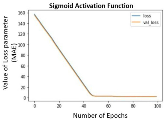
Figure 3.
Training and Validation loss curves while training of the model using sigmoid activation function (x-axis represents the number of successive epochs and y-axis holds the value of loss parameter (MAE) for each epoch).
Figure A1 shows the several iterations of training and validation loss curves depicting that the sigmoid activation function chosen in hidden layers and ReLU for the output layer performs well producing better-predicted elevation values for the plain terrain. Although other transfer functions are also converging well the trained model fails in giving good predictions on the new dataset as seen in the case of ReLU and TanH functions. The loss parameter values as derived from the usage of these activation functions are given in Table 2. The different model structure having indicated number of neurons in each layer (column 1) is analysed for training performance with different activation functions and the MAE, MSE and RMSE values are observed for selecting the best fit model. The best fit model architecture selected in this case is having 31-21-15-1 neurons in input- hidden layer 1- hidden layer 2- output layer respectively. The predictions from this model are assessed for accuracy by estimating its Root Mean Square Error (RMSE) with respect to TanDEM-X 90 m DEM on a new test area.

Table 2.
Value of Loss parameters for different activation functions in several iterations for Ghaziabad and surrounding regions (Plain Terrain).
5.1.2. ANN Model in MATLAB NN-Toolbox
A predictive elevation model is designed in the MATLAB NN-toolbox. The availability of more robust modelling and faster convergence algorithms makes the implementation of neural nets much simpler. The training, target and testing datasets are imported into the workspace in the matrix form. The training samples are comprised of the DEM elevation values and other geometrical parameters. The target samples include the corresponding elevation values from ICESat-2 footprints over the study area. The input feature vector that is the complete dataset is divided randomly into Train:Validation:Test in the ratio of 70:15:15 data samples respectively using the default function “dividerand”. The testing dataset is prepared from the subset of the study area for testing the performance of the trained model. The suitable model architecture is designed by selecting various model parameters such as the type of network used, training function, loss parameter, number of hidden layers and the appropriate activation functions. The Plain terrain of Ghaziabad and surrounding regions is aptly modelled using two hidden layers with 21 and 10 units in each of them respectively. The TRAINLM algorithm is used for the training of a Feed-Forward Backpropagation neural network, with a Log-sigmoid activation function.
The architecture of the best fit model is shown in Figure 4a. The training process of the model can be visualised in the network parameters window (Figure 4b). The best performance during training is depicted in the performance plot which shows the training, validation, test and best performance curves in an epoch (depicted on the x-axis) vs. MSE (depicted on the y-axis) of the plot (Figure 4c). The best performance is achieved at the 6th epoch with an MSE of 7.33 m. The training state having gradient, momentum constant (Mu) and validation checks are shown in relation to the number of epochs given on the x-axis for each parameter plot (Figure 4d). Mu (μ or Momentum update) also known as the control or adaptation parameter used in the Levenberg Marquardt training algorithm while updating the parameters that approximate the inverse of the Hessian matrix [35]. The regression plot of training vs. output is also available to check the distribution of data (Figure 4e).
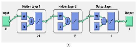
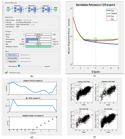
Figure 4.
ANN Model in MATLAB for Ghaziabad and surrounding regions: (a) Model Architecture; (b) Model Parameters, (c) Model training performance, (d) Training state of Model and (e) Regression plots for target vs. output values.
After the model is trained successfully, it is simulated on the test dataset of the area; these predictions, output and errors so produced, can be exported and saved. The output of DEM fusion from the models is assessed with accurate TanDEM-X 90 m DEM. The Fused Output DEM obtained from the ANN model in plain terrain of Ghaziabad and surrounding regions is represented in the map (Figure 5).
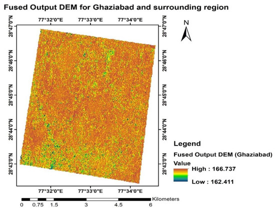
Figure 5.
Fused Output DEM obtained from Neural Network based fusion approach for Ghaziabad and surrounding regions.
The statistical analysis of the fused DEMs with the TanDEM-X 90 m DEM reveals that the fused DEMs have attained better RMSE values in comparison to the individual input DEMs. The fused DEMs obtained from the neural network model depict remarkable improvement by learning the relation of the elevation values with other topographical attributes. The RMSE has reduced significantly to 3.46 m (for the ANN model in Keras, Google Colab) and 4.34 m (from the ANN model in MATLAB NN-Toolbox) for the fused outputs from Neural Network models in plain areas. The percentage improvement obtained in Fused DEMs over the input DEMs is around 94.65% (Table 3). The Neural Network-based fusion approach is very efficient in executing its adaptive learning capability by modelling the relationship between the various input features and derived parameters with the precise reference ICESat-2 elevations. The input InSAR DEMs has improved in the plain terrain area with the use of ICESat-2 photon data.

Table 3.
Results for ANN fusion approach for Fused DEM assessed with TanDEM-X 90 m DEM in Ghaziabad and surrounding regions.
5.2. Results for Neural Network-Based Fusion Approach in Dehradun and Surrounding Region
5.2.1. ANN Model in Keras
Similar to in case of the first study area, for this hilly terrain of Dehradun and surrounding regions a sequential model with dense class layers is developed. Here, a greater number of units are required in the hidden layers to model the hilly undulating terrain having large variations in elevation values. A similar framework is designed as in the first study area using four layers, with MAE as loss parameter and Adam optimizer. The structure used for modelling the hilly region requires 31-64-128-1 neuron units in input- hidden layer 1- hidden layer 2- output layers respectively. Heuristics are applied and hyperparameter tuning is performed to determine the best fit model [33]. The hilly region of Dehradun and the surrounding regions has a total of 3423 samples, out of which 2396 are used as training data and 1027 samples as testing/validation data for the model. The training dataset contains the values of multiple DEM elevation values with slope, aspect, TPI, TRI and VRM in different land use land cover classes. Reference elevations are provided by the ICESat-2 footprints. The training performance of the neural networks with TanH activation functions giving a best fit model for this study site is depicted in the training loss and validation loss curves Figure 6.
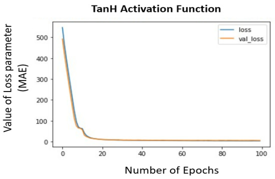
Figure 6.
Training and Validation loss curves while training the model using TanH activation function (x-axis represents the number of successive epochs and the y-axis holds the value of loss parameter (MAE) for each epoch).
The different transfer functions used for the training of the model in the heuristic approach are visualised in training and validation loss curves (Appendix A, Figure A2). Table 4 represents the values of loss parameters obtained by using different activation functions for the Dehradun region. The first column represents the architecture of the model with number of neurons in each layer and further columns represents the loss parameter values for sigmoid, ReLU and TanH activation function. TanH function performs well for this region in training and validation but predictions over the new testing dataset were not satisfactory. Similarly, for ReLU and Sigmoid functions, the predictions obtained for the fused DEMs are not appropriate to be used further.

Table 4.
Value for Loss parameters for different activation functions in several iterations for Dehradun and surrounding regions (Hilly region).
5.2.2. ANN Model in MATLAB NN-Toolbox
An effective and robust model is designed in the MATLAB NN-Toolbox for the Hilly terrain of Dehradun and the surrounding regions. The training samples comprised of DEM elevation values with other geometrical features, target elevations provided from the ICESat-2 ATL08 data and the testing data are prepared from the subset of the study area. Using the faster converging algorithm TRAINLM along with a structure of 31-64-128-1 is used. More units are required in this type of terrain as found during the study. The PURELIN transfer function is most suitable providing a larger range of output values in contrast to sigmoid functions [35]. The model architecture used for this study area is shown in Figure 7a and it requires more neurons to model this terrain in comparison to the plain terrain of the Ghaziabad region. The model parameters selected for modelling this area are shown in Figure 7b. The best training performance of the model is achieved at the 6th epoch (Figure 7c) showing the train, test, validation and best performance curves in relation to the number of epochs as represented on the x-axis of this plot. The training state in terms of gradient, Mu and validation checks in relation to the number of epochs is depicted in Figure 7d and the regression plot between the target and output values is plotted below (Figure 7e).
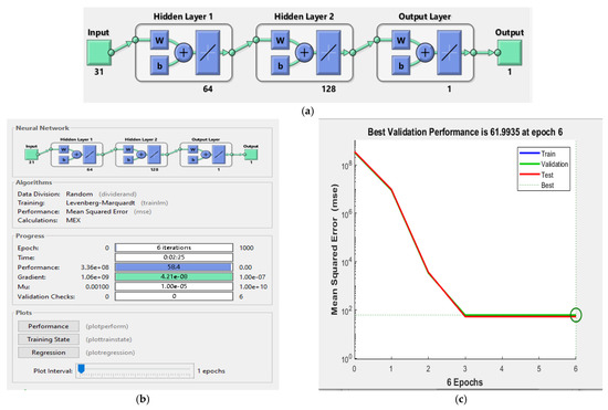
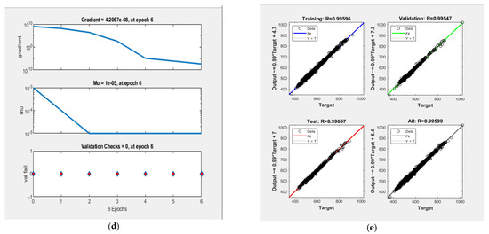
Figure 7.
ANN Model in MATLAB for Dehradun and surrounding regions: (a) Model Architecture; (b) Model Parameters, (c) Model training performance, (d) Training state of Model and (e) Regression plots for target vs. output values.
The predictions for fused DEMs are assessed with the TanDEM-X 90 m DEM to check the accuracy of the results. The fused output DEM from the Neural Networks predictive modelling is shown in the map (Figure 8). The 3D view for visualization of the terrain is depicted in Figure 9. The Root Mean Square Error (RMSE) is estimated to analyze the accuracy of fused DEMs in comparison to the multiple-input DEMs (Table 5).
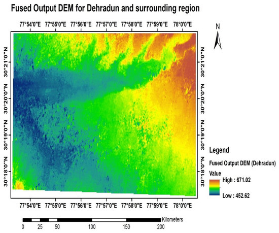
Figure 8.
Fused Output DEM obtained from Neural Network-based fusion approach for Dehradun and surrounding regions.
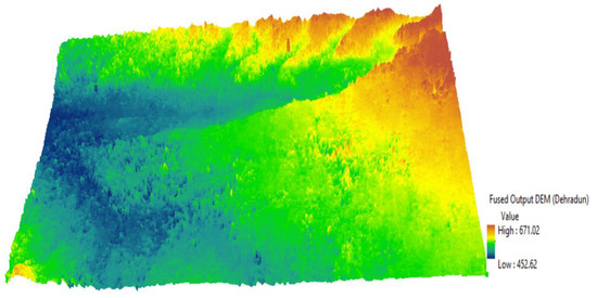
Figure 9.
Fused Output DEM (3D view) for Dehradun and surrounding regions for the depiction of terrain.

Table 5.
Results for ANN fusion approach for Fused DEM assessed with TanDEM-X 90 m DEM in Dehradun and surrounding regions.
The Neural Network-based fusion approach for DEM improvement is implemented in the hilly terrain of Dehradun and surrounding regions. The designed network is trained successfully and the resultant fused DEMs show a significant improvement in this region also. The predicted fused elevations have attained an RMSE of 10.95 m which is very low in comparison to all the individual input InSAR DEMs, for the highly undulating terrain of Dehradun and its surroundings. Moreover, the percentage improvement of 82.62% over the input DEM is achieved in the hilly region which is a highly considerable amount of improvement in such an undulating terrain. Thus, the neural network-based fusion framework is found efficient and successful in hilly terrains which have dense forests and variable slopes across the region. Although, modelling such a difficult terrain with a neural network-based fusion method requires proper data preparation and a large number of iterations for designing the best fit model.
6. Discussion
The objective of DEM improvement by using a novel neural network-based fusion approach is implemented successfully for two different types of geographic terrains in the Indian Region. The important criteria to be considered while selection of InSAR image pairs for the study sites was discussed and the InSAR DEMs generated for the two study regions were generated by selecting the SAR images based on baselines and coherence information. More is the quality of input SAR images for DEMs, the better quality of InSAR DEMs will be produced and the topographic information retrieved from them will be more appropriate. Further, the relation of various DEM derivatives such as slope, aspect, TPI, TRI and VRM parameters with the DEM accuracy were thoroughly studied and discussed; these parameters affect the DEM quality as given in the literature survey and hence, validate their use in the development of a fusion framework with the support of a neural network. ANN being a mathematically computational and non-parametric model, it can handle the complex non-linear dataset; this idea is used as a base for developing a fusion framework using neural network-based models. Along with the input DEMs elevations, some derived geometrical spatial features are useful in building a robust relationship between the reference and the predicted elevations from the model. The two study sites selected for our study comprise diverse topography and varying landforms. The uncertainty in the values of land and canopy heights from the ICESat-2 ATL08 data products are very important to be considered while data preparation and pre-processing steps. The neural network predictive modelling for both terrains requires a different type of heuristics to be applied for obtaining the best fit or an efficient trained model. The activation functions, number of hidden layers and the number of neurons in the hidden layers are the crucial parameters which need to be considered for designing the most suitable architecture of the neural network. The results obtained from the neural network models for both types of terrain indicated considerable improvement in the fused output DEMs in comparison to the input InSAR DEMs. The RMSE obtained from the height error estimation with the TanDEM-X 90 m DEM is significantly reduced for the plain-urban type of topography as well as for hilly undulating terrain with dense forest covers. The InSAR DEMs are improved largely in a plain area with an RMSE of 3.46 m while in a hilly area value of RMSE is 10.95 m. The improvement is more in the plain region as compared to the hilly region but overall fused DEMs obtained from the models are improved when compared with the input DEMs in both regions.
7. Conclusions
A novel approach of fusion developed with data-driven neural network models is successful and highly efficient in improving the InSAR-based DEMs in the plain and hilly terrains of Indian regions. The study results inferred the implementation of this approach was very successful in both the study areas. The important conclusion drawn from the study is that important factors such as the baselines and coherence information play a crucial role in the selection of interferometric pairs from the space-borne SAR sensors. The quality of InSAR DEMs is further improved by combining information from multiple input elevations of InSAR DEMs, derived topographical attributes and their relationship with the precise ICESat-2 altimetry data in a neural net-based fusion approach. Heuristics are applicable for obtaining the appropriate model architecture for both the study areas. The hyperparameter tuning or optimization helps in selecting the suitable model parameters and the activation functions in a faster way. Training performance curves are important in visualizing the model training and obtaining the best fit models. The results from the trained models on a new dataset from test areas showed a remarkable improvement in the fused DEMs in terms of RMSE parameters. The developed models performed effectively well in obtaining improved and better accuracy DEMs in the plain and hilly terrains.
Author Contributions
Conceptualization, P.G. and A.B.; methodology, P.G. and A.B.; software, P.G.; validation, A.B. and P.G.; formal analysis, P.G. and A.B.; investigation, P.G. and A.B.; resources, P.G. and A.B.; data curation, P.G.; writing- original draft preparation, P.G.; writing- review, A.B. and editing, P.G. and A.B.; visualization, P.G. and A.B.; supervision, A.B. All authors have read and agreed to the published version of the manuscript.
Funding
This research received no external funding.
Institutional Review Board Statement
Not applicable.
Informed Consent Statement
Not applicable.
Data Availability Statement
All the datasets used in this study are available in public domain and are openly accessible. The Sentinel- 1A/1B, Sentinel- 2A, ICESat-2 ATL08 product, TanDEM-X 90 m DEM and SOI Toposheets can be found at: https://scihub.copernicus.eu/dhus/#/home (accessed on 15 September 2021), https://openaltimetry.org/data/icesat2/ (accessed on 20 October 2021), https://download.geoservice.dlr.de/TDM90/ (accessed on 24 December 2021), and https://onlinemaps.surveyofindia.gov.in/FreeMapSpecification.aspx (accessed on 30 October 2021) respectively. The selection of SAR image pairs is based on Baseline Tool available at https://search.asf.alaska.edu/#/?searchType=Baseline%20Search (accessed on 13 September 2021). The Google Earth Pro is used for data visualization required in the preparation of LULC maps and locating footprints of ICESat-2 on generated InSAR DEMs.
Acknowledgments
The authors are thankful to ISRO (Indian Space Research Organization), ESA (European Space Agency), DLR (German Space Agency), NASA (National Aeronautics and Space Administration), ASF (Alaska Satellite Facility), SOI (Survey of India) and Google LLC for their valuable support to the researchers in providing openly accessible data and detailed specifications about them. The authors are highly grateful to the Director, IIRS for providing technical expertise, lab facilities and encouragement for conducting research studies at Indian Institute of Remote Sensing.
Conflicts of Interest
The authors declare no conflict of interest.
Appendix A
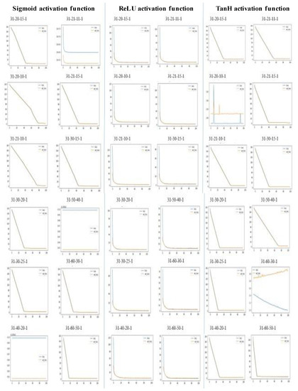
Figure A1.
Training loss and Validation loss curves depicting the training performance of the models with three different activation functions for Ghaziabad and surrounding regions.
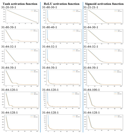
Figure A2.
Training loss and Validation loss curves depicting the training performance of the models with three different activation functions for Dehradun and surrounding regions.
References
- Miller, C.L.; Laflamme, R.A. The digital terrain model-Theory & Application. Am. Soc. Photogramm. 1958, XXIV, 11. [Google Scholar]
- Li, J.; Wong, D.W. Effects of DEM sources on hydrologic applications. Comput. Environ. Urban Syst. 2010, 34, 251–261. [Google Scholar] [CrossRef]
- Song, X.; Qi, Z.; Du, L.P.; Kou, C.L. The Influence of DEM Resolution on Hydrological Simulation in the Huangshui River Basin. Adv. Mater. Res. 2012, 518, 4299–4302. [Google Scholar] [CrossRef]
- Khojeh, S.; Ataie-Ashtiani, B.; Hosseini, S.M. Effect of DEM resolution in flood modeling: A case study of Gorganrood River, Northeastern Iran. Nat. Hazards 2022, 112, 2673–2693. [Google Scholar] [CrossRef]
- Louise, A.J.v.; Keiko, S.; Michel, M.; Don, M. Digital Elevation Models. 2007. Available online: http://hdl.handle.net/10986/34445 (accessed on 18 October 2021).
- Woodhouse, I.H. Introduction to Microwave Remote Sensing; TayloCRC & FPrancies Group: Boca Raton, FL, USA, 2006. [Google Scholar]
- Massonnet, D.; Feigl, K.L. Radar interferometry and its application to changes in the Earth’s surface. Rev. Geophys. 1998, 36, 441–500. [Google Scholar] [CrossRef]
- Ferretti, A.; Monti-guarnieri, A.; Prati, C.; Rocca, F.; Massonnet, D. InSAR Principles: Guidelines for SAR Interferometry Processing and Interpretation; European Space Agency: Paris, France, 2007. [Google Scholar]
- Michelle Sneed, “Interferometric Synthetic Aperture Radar (InSAR)”, USGS, Land Subsidence in California. 2018. Available online: https://www.usgs.gov/centers/ca-water-ls/science/interferometric-synthetic-aperture-radar-insar?qt-science_center_objects=0#qt-science_center_objects (accessed on 7 September 2021).
- Fukumori, I. Data Assimilation by Models. In International Geophysics; Academic Press: Cambridge, MA, USA, 2001; pp. 237–265. [Google Scholar]
- Kim, D.E.; Liong, S.-Y.; Gourbesville, P.; Andres, L.; Liu, J. Simple-Yet-Effective SRTM DEM Improvement Scheme for Dense Urban Cities Using ANN and Remote Sensing Data: Application to Flood Modeling. Water 2020, 12, 816. [Google Scholar] [CrossRef]
- Papasaika, H.; Poli, D.; Baltsavias, E. Fusion of Digital Elevation Models from Various Data Sources. In Proceedings of the 2009 International Conference on Advanced Geographic Information Systems & Web Services, Cancun, Mexico, 1–7 February 2009; pp. 117–122. [Google Scholar] [CrossRef]
- Fuss, C.E. Digital Elevation Model Generation and Fusion. Master’s Thesis, The University of Guelph, Guelph, ON, Canada, 2013; p. 159. Available online: https://atrium.lib.uoguelph.ca/xmlui/bitstream/handle/10214/7571/Fuss_Colleen_201309_Msc.pdf?sequence=3 (accessed on 21 October 2021).
- Papasaika, H.; Kokiopoulou, E.; Baltsavias, E.; Schindler, K.; Kressner, D. Fusion of Digital Elevation Models Using Sparse Representations. In ISPRS Conference on Photogrammetric Image Analysis; Springer: Berlin/Heidelberg, Germany, 2011; Volume 6952, pp. 171–184. [Google Scholar] [CrossRef]
- Yousif, H.; Li, J.; Chapman, M.; Shu, Y. Accuracy Enhancement of Terrestrial Mobile LiDAR Data Using Theory of Assimilation. Int. Arch. Photogramm. Remote Sens. Spat. Inf. Sci. 2010, XXXVIII, 639–645. [Google Scholar]
- Bhardwaj, A.; Jain, K.; Chatterjee, R.S. Generation of high-quality digital elevation models by assimilation of remote sensing-based DEMs. J. Appl. Remote Sens. 2019, 13, 044502. [Google Scholar] [CrossRef]
- Bagheri, H.; Schmitt, M.; Zhu, X.X. Fusion of TanDEM-X and Cartosat-1 elevation data supported by neural network-predicted weight maps. ISPRS J. Photogramm. Remote Sens. 2018, 144, 285–297. [Google Scholar] [CrossRef]
- Girohi, P.; Bhardwaj, A. Improving SAR Interferometry based Digital Elevation Models using Successive Best Pixel Selection Approach for DEM fusion. In Abstract Booklet NSSS 2022; IISER Kolkata: Haringhata, India, 2022; p. 119. [Google Scholar]
- Kulp, S.A.; Strauss, B.H. CoastalDEM: A global coastal digital elevation model improved from SRTM using a neural network. Remote Sens. Environ. 2018, 206, 231–239. [Google Scholar] [CrossRef]
- Kampüs, K. Estimation of Unknown Height With Artificial Neural Network on Digital Terrain Model. Int. Arch. Photogramm. Remote Sens. Spat. Inf. Sci. 2002, 115–118. Available online: http://www.isprs.org/congresses/beijing2008/proceedings/3b_pdf/21.pdf (accessed on 7 December 2021).
- Nguyen, N.S.; Kim, D.E.; Jia, Y.; Raghavan, S.V.; Liong, S.Y. Application of Multi-Channel Convolutional Neural Network to Improve DEM Data in Urban Cities. Technologies 2022, 10, 61. [Google Scholar] [CrossRef]
- Kim, D.; Liu, J.; Liong, S.-Y.; Gourbesville, P.; Strunz, G. Satellite DEM Improvement Using Multispectral Imagery and an Artificial Neural Network. Water 2021, 13, 1551. [Google Scholar] [CrossRef]
- Tian, X.; Shan, J. Comprehensive Evaluation of the ICESat-2 ATL08 Terrain Product. IEEE Trans. Geosci. Remote Sens. 2021, 59, 8195–8209. [Google Scholar] [CrossRef]
- Brown, M.E.; Arias, S.D.; Neumann, T.; Jasinski, M.F.; Posey, P.; Babonis, G.; Glenn, N.F.; Birkett, C.M.; Escobar, V.M.; Markus, T. Applications for ICESat-2 Data: From NASA’s Early Adopter Program. IEEE Geosci. Remote Sens. Mag. 2016, 4, 24–37. [Google Scholar] [CrossRef]
- Wang, C.; Zhu, X.; Nie, S.; Xi, X.; Li, D.; Zheng, W.; Chen, S. Ground elevation accuracy verification of ICESat-2 data: A case study in Alaska, USA. Opt. Express 2019, 27, 38168–38179. [Google Scholar] [CrossRef]
- Zhang, Y.; Pang, Y.; Cui, D.; Ma, Y.; Chen, L. Accuracy Assessment of the ICESat-2/ATL06 Product in the Qilian Mountains Based on CORS and UAV Data. IEEE J. Sel. Top. Appl. Earth Obs. Remote Sens. 2020, 14, 1558–1571. [Google Scholar] [CrossRef]
- Bhardwaj, A. Investigating the Terrain Complexity from ATL06 ICESat-2 Data for Terrain Elevation and Its Use for Assessment of Openly Accessible InSAR Based DEMs in Parts of Himalaya’s. Eng. Proc. 2021, 10, 65. [Google Scholar] [CrossRef]
- Carabajal, C.C.; Harding, D.J. ICESat validation of SRTM C-band digital elevation models. Geophys. Res. Lett. 2005, 32, 1–5. [Google Scholar] [CrossRef]
- Goud, G.P.S.; Bhardwaj, A. Estimation of Building Heights and DEM Accuracy Assessment Using ICESat-2 Data Products. Eng. Proc. 2021, 10, 37. [Google Scholar] [CrossRef]
- Dandabathula, G.; Sitiraju, S.R.; Jha, C.S. Retrieval of building heights from ICESat-2 photon data and evaluation with field measurements. Environ. Res. Infrastruct. Sustain. 2021, 1, 011003. [Google Scholar] [CrossRef]
- Hu, Y.H.; Hwang, J.N. Handbook of Neural Network Signal Processing; Academic Press, Inc.: San Diego, NY, USA, 2001. [Google Scholar]
- Anderson, J.A. Introduction to Neural Networks, 8th ed.; MIT Press: Cambridge, MA, USA, 1994; Volume 6. [Google Scholar]
- Kanungo, D.; Arora, M.; Sarkar, S.; Gupta, R. A comparative study of conventional, ANN black box, fuzzy and combined neural and fuzzy weighting procedures for landslide susceptibility zonation in Darjeeling Himalayas. Eng. Geol. 2006, 85, 347–366. [Google Scholar] [CrossRef]
- Kavzoglu, T.; Mather, P.M. The use of backpropagating artificial neural networks in land cover classification. Int. J. Remote Sens. 2003, 24, 4907–4938. [Google Scholar] [CrossRef]
- Demuth, H.; Beale, M. Neural Network Toolbox Version4. In Networks; MathWorks: Portola Valley, CA, USA, 2002; Volume 24, No. 1, pp. 1–8. Available online: http://citeseerx.ist.psu.edu/viewdoc/download?doi=10.1.1.123.6691&rep=rep1&type=pdf (accessed on 2 January 2022).
- Braun, A. Retrieval of digital elevation models from Sentinel-1 radar data–open applications, techniques, and limitations. Open Geosci. 2021, 13, 532–569. [Google Scholar] [CrossRef]
- Toutin, T. Impact of terrain slope and aspect on radargrammetric DEM accuracy. ISPRS J. Photogramm. Remote Sens. 2002, 57, 228–240. [Google Scholar] [CrossRef]
- Riley, R.E.S.J.; De Gloria, S.D. Terrain Ruggedness Index- Riley.pdf. Intermt. J. Sci. 1999, 5, 23–27. [Google Scholar]
- Weiss, A. Topographic Position and Landforms Analysis. In Proceedings of the Poster Presentation, ESRI User Conference, San Diego, CA, USA, 2001; Volume 64, pp. 227–245. Available online: http://scholar.google.com/scholar?hl=en&btnG=Search&q=intitle:Topographic+Position+and+Landforms+Analysis#0 (accessed on 18 March 2022).
- Jenness, J. Topographic Position Index (tpi_jen.avx). 2006. Available online: http://www.jennessent.com/arcview/tpi.html (accessed on 20 March 2022).
- Sappington, J.M.; Longshore, K.M.; Thompson, D.B. Quantifying Landscape Ruggedness for Animal Habitat Analysis: A Case Study Using Bighorn Sheep in the Mojave Desert. J. Wildl. Manag. 2007, 71, 1419–1426. [Google Scholar] [CrossRef]
- Wessel, B.; Huber, M.; Wohlfart, C.; Marschalk, U.; Kosmann, D.; Roth, A. Accuracy assessment of the global TanDEM-X Digital Elevation Model with GPS data. ISPRS J. Photogramm. Remote Sens. 2018, 139, 171–182. [Google Scholar] [CrossRef]
- Kumar, P.; Bhattacharya, B.K.; Pal, P. Impact of vegetation fraction from Indian geostationary satellite on short-range weather forecast. Agric. For. Meteorol. 2012, 168, 82–92. [Google Scholar] [CrossRef]
- Kirthiga, S.M.; Patel, N.R. Impact of updating land surface data on micrometeorological weather simulations from the WRF model. Atmosfera 2018, 31, 165–183. [Google Scholar] [CrossRef]
- Dolloff, J.; Carr, J. Computation of scalar accuracy metrics LE, CE, and SE as both predictive and sample-based statistics. In Proceedings of the ASPRS 2016 Annual Conference and Co-Located JACIE Workshop-Imaging Geospatial Technol. Forum Co-Located JACIE Work, Fort Worth, TX, USA, 11–15 April 2016; pp. 1–15. [Google Scholar]
Publisher’s Note: MDPI stays neutral with regard to jurisdictional claims in published maps and institutional affiliations. |
© 2022 by the authors. Licensee MDPI, Basel, Switzerland. This article is an open access article distributed under the terms and conditions of the Creative Commons Attribution (CC BY) license (https://creativecommons.org/licenses/by/4.0/).