Minimally Distorted Adversarial Images with a Step-Adaptive Iterative Fast Gradient Sign Method

Abstract

The safety and robustness of convolutional neural networks (CNNs) have raised increasing concerns, especially in safety-critical areas, such as medical applications. Although CNNs are efficient in image classification, their predictions are often sensitive to minor, for human observers, invisible modifications of the image. Thus, a modified, corrupted image can be visually equal to the legitimate image for humans but fool the CNN and make a wrong prediction. Such modified images are called adversarial images throughout this paper. A popular method to generate adversarial images is backpropagating the loss gradient to modify the input image. Usually, only the direction of the gradient and a given step size were used to determine the perturbations (FGSM, fast gradient sign method), or the FGSM is applied multiple times to craft stronger perturbations that change the model classification (i-FGSM). On the contrary, if the step size is too large, the minimum perturbation of the image may be missed during the gradient search. To seek exact and minimal input images for a classification change, in this paper, we suggest starting the FGSM with a small step size and adapting the step size with iterations. A few decay algorithms were taken from the literature for comparison with a novel approach based on an index tracking the loss status. In total, three tracking functions were applied for comparison. The experiments show our loss adaptive decay algorithms could find adversaries with more than a 90% success rate while generating fewer perturbations to fool the CNNs.

1. Introduction

Convolutional neural networks (CNNs) are popular to perform image recognition tasks because CNNs can automatically learn the visual features from images or videos. In previous research, these visual features are mostly handcrafted, potentially losing significant information in the feature extraction process [1]. The CNNs overcame these limitations and dramatically improved the efficiency of classifying images. However, the performance of CNNs is highly influenced by the image quality, object visibility, and other conditions during training [1]. For instance, in a medical application, such as recognizing the surgical tools in laparoscopic surgery video streams, some visual challenges highly influence the CNNs’ performance for object classification [1,2]. These visual challenges are quite common in real medical applications, i.e., the surgical tools may be occluded by tissue or smoke may be generated during surgery, lenses are stained by blood, and motion blur is caused by movement or unstable camera position [1]. All these challenges threaten the CNNs’ performance, making it difficult to recognize the surgical tool under these challenging conditions. In addition, even a well-trained CNN can be easily confused by some slight modifications added to legitimate images, and this vulnerability to adversarial samples generalizes over all CNN architectures [2,3,4,5,6]. Therefore, some efforts need to be spent to improve the model’s resilience to these adversarial perturbations.

Adversarial images can be easily generated by flipping the image [7] or adding invisible perturbations to the original input [3,4,5,6,8]. An efficient, targeted way to generate adversarial image perturbations is backpropagating the loss gradient as a directed modification to the input images [3,4,5,6,8,9]. The fast gradient sign method (FGSM) was first proposed in [9], modified by incorporating extension methods, such as iteratively applying the FGSM on the input [10], by adding momentum to the gradient (MI-FGSM) [11], or by projecting the perturbation back to max norm box after every iteration (PGD) [12]. There were further methods published that use the forward derivative to construct adversarial saliency maps [13] or generative adversarial networks (GANs) [14].

To analyze convolution neural network robustness to these adversarial images, usually, a max norm constraint is assigned to the amplitude of perturbation. A high error rate on these adversarial images indicates less robustness in convolution neural network classification. Usually, as the amplitude of perturbation increases, the error rate is increases too. But, the opposite, i.e., a measure based on a minimal perturbation, is sufficient for the model to misclassify an input is another interesting direction. Related work can be found in the literature, such as constructing the provably minimally distorted adversarial examples with formal verification approaches [15], using fast adaptive boundary attacks to generate minimally distorted adversarial examples [16], using an extremely limited scenario that only modifies one pixel, which was proposed in [17], establishing an optimization model to generate an adversary with controllable amplitude [18], and using an adaptive learning rate to influence the modification [19].

This paper provides the following contributions:

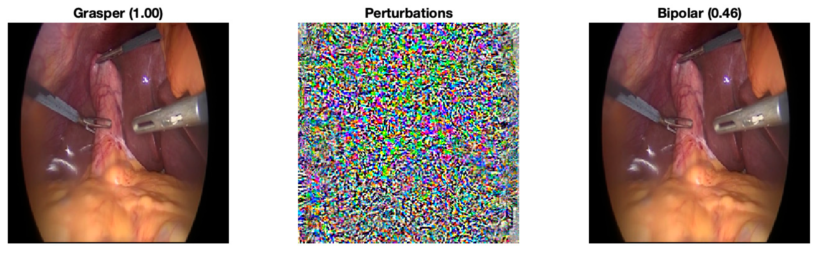
• We propose the step size adaptive i-FGSM to generate adversaries with fewer perturbations. Initially, the classic fast gradient sign method (FGSM) was applied to seek a minimum perturbation individually for each input that is sufficient to change the model decision. When the size of the perturbation is not large enough to change prediction, the algorithm leads to an iterative form (i-FGSM) until the input is misclassified. This method is rather crude and usually lacks a minimal solution. Therefore, we modified this minimum search and formulated an adaptive gradient descent problem [19]. To solve this problem, this paper further extends the method from our previous work in [19].
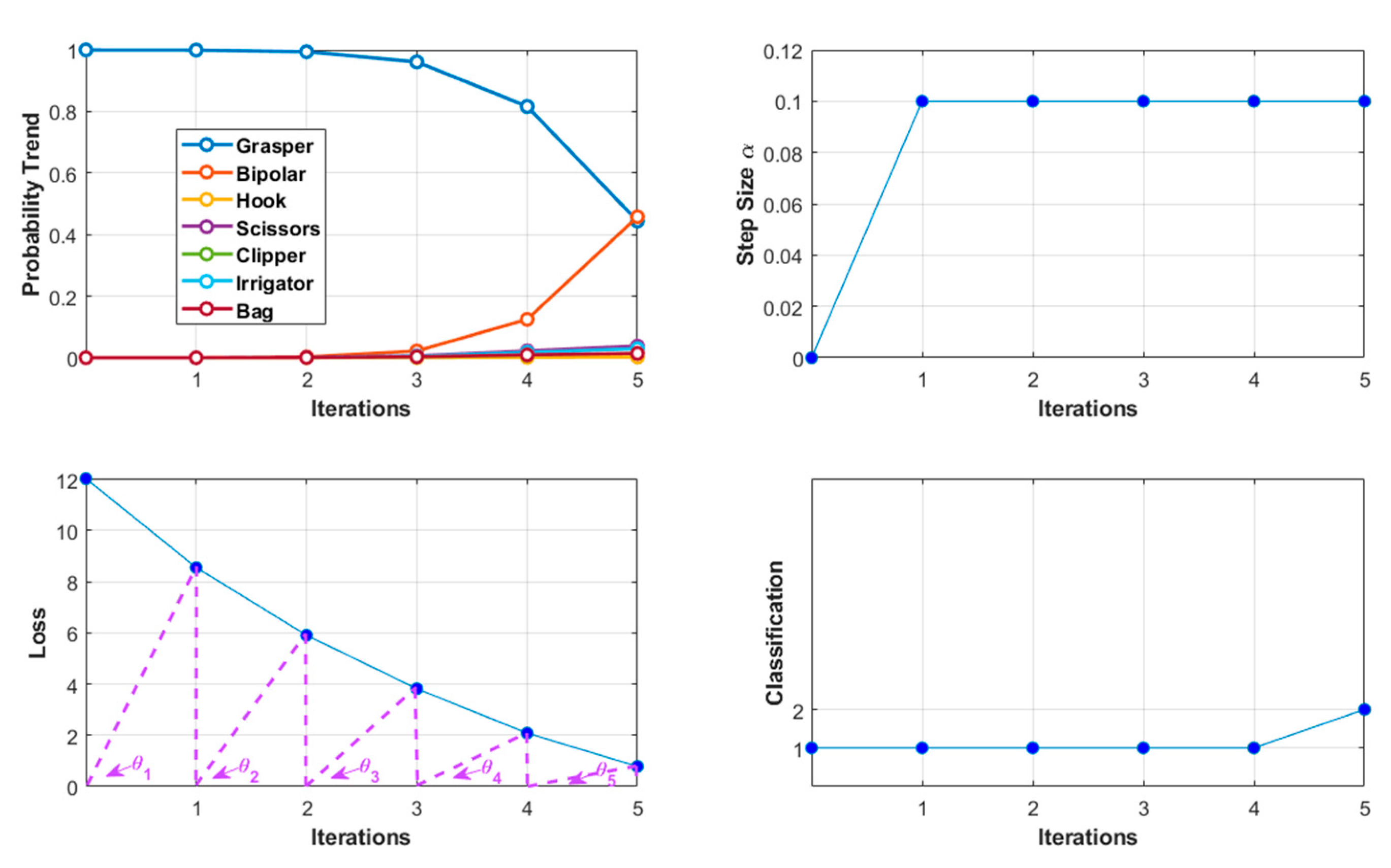
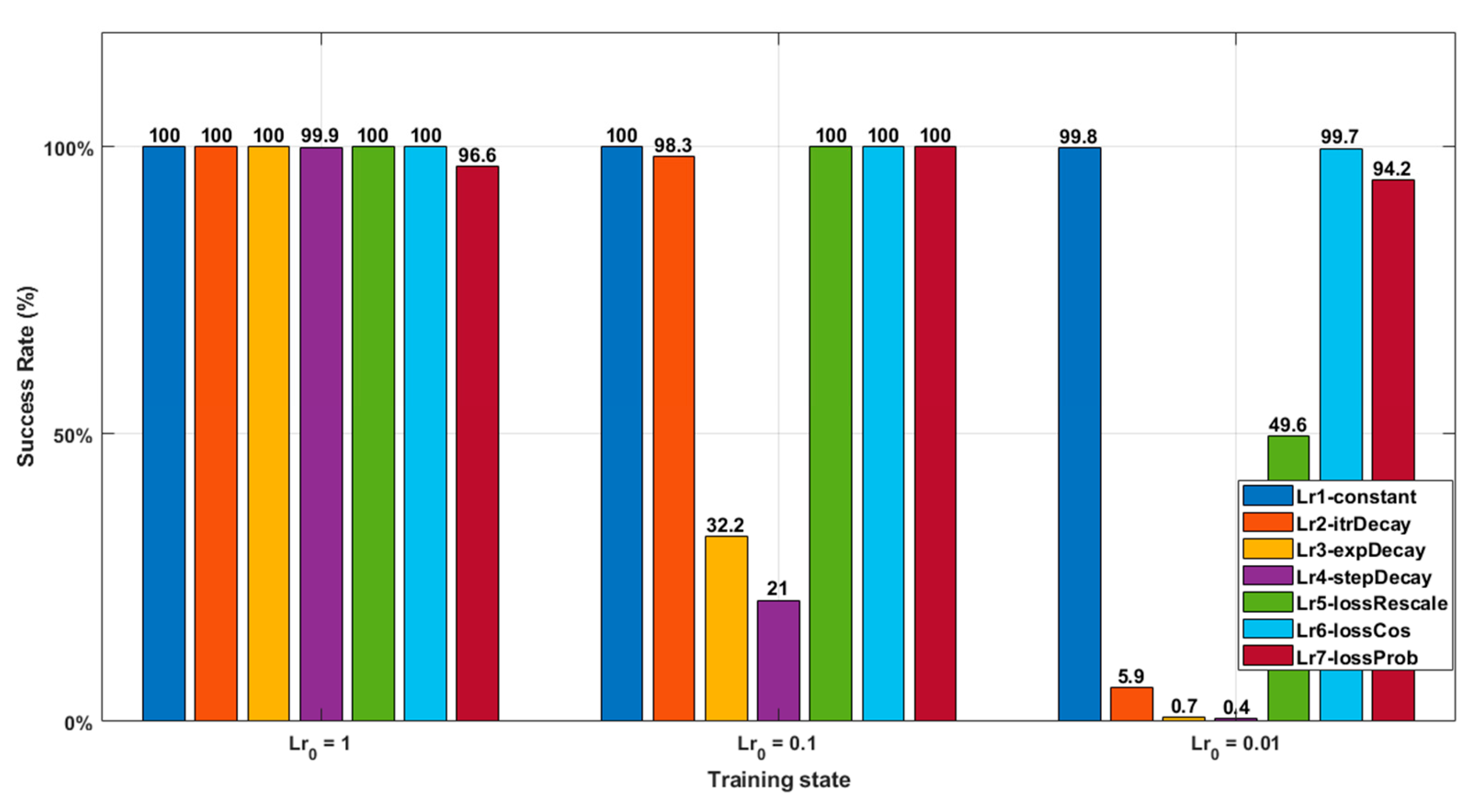
• We introduce a loss adaptive algorithm to adjust the step size. Three decay algorithms from the literature were applied to the step size (or learning rate in the context of machine learning). Additionally, we also introduce a novel decay algorithm that keeps track of the loss of the current iteration and uses it as feedback to adjust the step size for the next iteration. In total, there are three different loss-tracking functions: the loss rescale function, loss trigonometric function, and loss-related original classification probability.
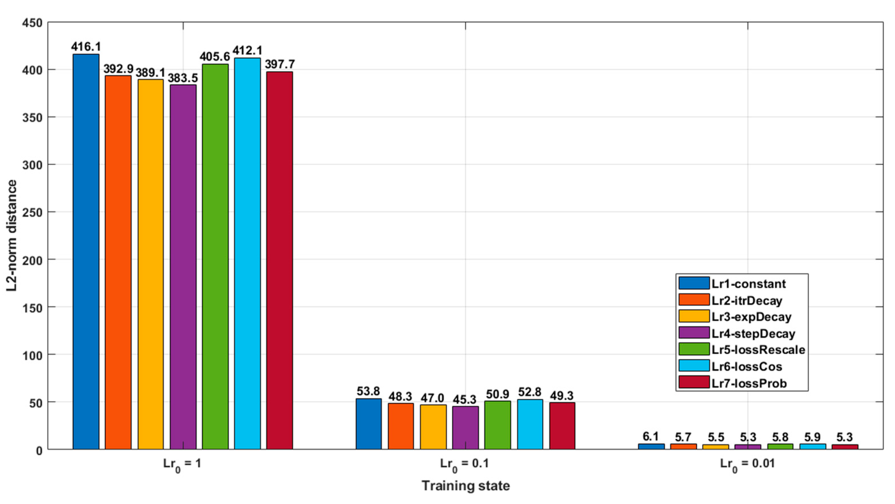
• We provide the experimental results that indicate the influence of different step sizes in the adversary-generated process. The experiment includes two parts. Depending on whether a target classification is given, i.e., the adversary can be generated by moving the input away from its original classification or moving the input close to a target classification. The experimental results illustrate that our loss adaptive step size algorithms could efficiently generate adversaries with fewer perturbations while maintaining a high adversarial success rate.

This paper is organized into the following sections. Section 1 introduced the importance of CNN safety in medical applications and how to generate adversaries with minimal distortion to fool a CNN. Section 2 presents the experiment setting, the minimal-distorted adversary generate technique, the algorithms, including different step size reduce functions, and the adversary evaluation metric. Section 3 provides the result of a target adversarial attack and non-target adversarial attack. Section 4 discusses the limitations of the adversary-generated algorithms. Section 5 concludes with the contribution of this research.

2. Methods

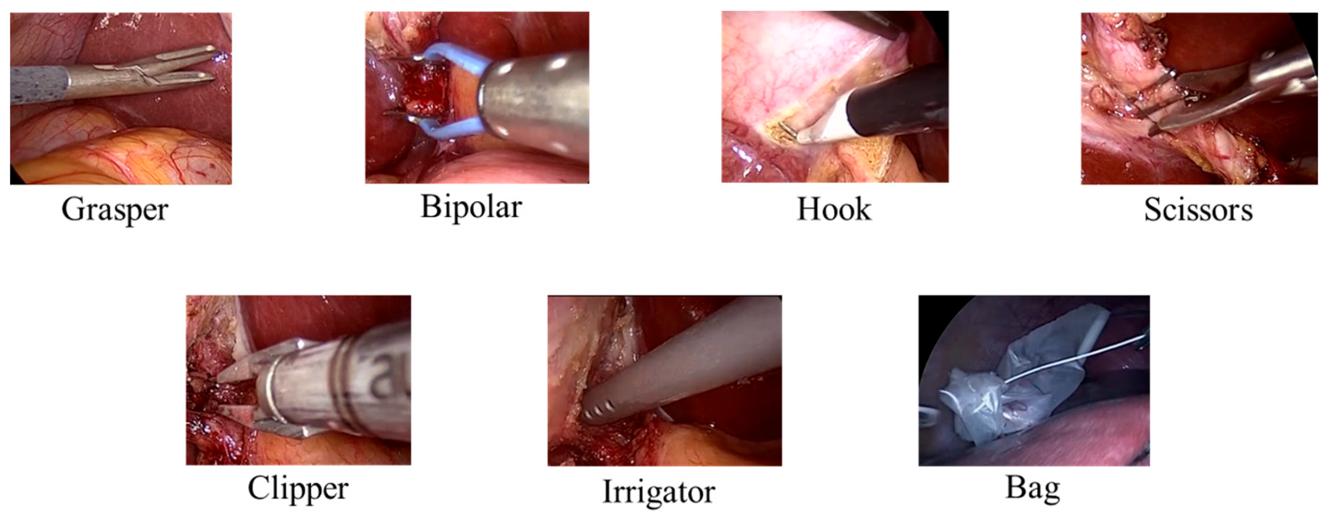
2.1. Material

In this study, our source dataset is the Cholec80 dataset [1], which contains 80 cholecystectomy videos, in which 7 surgical tools were used (see Figure 1), making up 7 different classes (

Table 1. The class index, corresponding surgical tool, and the number of frames in the derived 1-class dataset.

Class	Surgical Tool	Number of Frames
1	Grasper	23,507
2	Bipolar	3222
3	Hook	44,887
4	Scissors	1483
5	Clipper	2647
6	Irrigator	2899
7	Bag	1545

) to be detected in video frames [19,20,21,22]. To fulfill the SoftMax requirements [23], only 1-class image frames are used in this study and were extracted from the dataset (in total 80,190 images). From this derived dataset, the first 40 videos (31,477 images) were used as the training set, and the remaining 40 videos (48,713 images) were used as the test set. The convolutional neural network model exemplarily used in this study is Resnet-50 [24]. Resnet-50 has a plain baseline network that starts with down-sampling convolution and four convolution blocks, and ends with average pooling layer, fully connected layer andSoftMax layer. The shortcut connections were inserted on the plain network to perform the residual learning reformulation [24]. The model was trained for 30 epochs. For adversarial perturbation evaluation, 200 correctly classified images of each class were randomly selected from the test set, i.e., in total, there were 1400 images used.

2.2. Adversarial Attack

As mentioned in the introduction, an ameliorated fast gradient sign method was applied to search for the adversary with minimal perturbations. If a one-step update cannot modify the input to another class, the program will automatically turn into basic iterative form (i-FGSM) until the classification changes (see Figure 2). For instance, the perturbation process can be started with a small amplitude and continuously applied to the input until the input is misclassified; the difference between the original input and the final adversary would be the smallest successful perturbation for this specific input. This smallest successful perturbation also represents a minimal safe area around the original input. However, the smallest successful perturbation depends not solely on the sample properties, such as whether it is close to a decision boundary, but is also influenced by the model performance, i.e., how well it approximates optimal decision boundaries. It is more difficult to fool a well-trained model than a less-trained model; different model architectures might reach different robustness levels to the perturbations. At the same time, the nonlinear optimization process in the high-dimensional input space (high-resolution images) is difficult to solve, as the gradient search is error prone and sensitive to step size and local minima.

It is practically not possible to explore the whole decision boundary around a class center for a minimal distance to the next class. Therefore, an approximate method is introduced that uses defined directions in the high-dimensional image space. The target adversarial attack is a gradient search minimizing the cross-entropy loss between model prediction and a chosen target class, i.e., it changes the image in the direction of the selected target class [10,19]. A non-target adversarial attack maximizes the cross-entropy loss of model prediction and original class, i.e., it implements the steepest ascent away from the current class center [9,10,19]. In both approaches, the final perturbation should be the closest successful perturbation in the relative direction. The cross-entropy loss is defined as follows:

$$J\left(\theta , x, y\right)=-{\sum }_{i=1}^{N}y·\log f_{\theta }\left(x\right)$$

(1)

where $\theta$ represents the model parameters, $N$ is the number of classes, $x$ is the input image presented to the model, $f_{\theta }\left(x\right)$ is the model prediction of $x$, and $y$ is the original label that was assigned to $x$ in case of a non-target attack or a target classification label that is used in a targeted attack.

If a target classification is chosen for an adversarial attack [10,19], the input is updated in every iteration following the gradient descent of $J\left(\theta , x, y\right)$, with $y$ representing the label of a target classification (class(x) ≠ y). The basic iterative fast gradient sign method (i-FGSM) is formulated as follows:

$$\begin{array}{c}{x}_0^{*}=x;\\ x_n^{*}=x_{n-1}^{*}-\alpha \left(\mathrm{n}\right)·\mathrm{sign} \left[{\nabla }_x J\left(\theta , x_{n-1}^{*}, y_{target}\right)\right];\end{array}$$

(2)

where $x_0^{*}$ is the original input image, $x_n^{*}$ is the generated adversarial image at the nth iteration, and $x_{n-1}^{*}$ is the generated adversarial image at the (n − 1)th iteration. $y_{target}$ is the chosen target label that must be different from the original class of image $x$. In this paper, α is initialized as a constant and is then modified to different functionals α(n) that adaptive to the iteration count. Thus, the step size of iterative image modifications is adjusted according to different decay algorithms, and their effect on the amplitude of perturbations is investigated, which is required to change the classification output. The final perturbation is the result of summing up the changes imposed in the iteration process and will be represented by $\delta$. The search process for the minimal perturbation ${\delta }^{*}$ can be described as a nonlinear optimization of Function (3) below, minimizing the cost until the classification changed to the target label.

$${\delta }^{*}=\underset{\delta }{\min }(\mathrm{argmin}J\left(\theta , x+\delta , y_{target}\right));$$

(3)

When the non-target adversarial attack is chosen, the input is updated by ascending the gradient of the original classification loss in order to change the model prediction to another classification label [9,10,19]. The iteration is described as follows:

$$\begin{array}{c}{x}_0^{*}=x;\\ x_n^{*}=x_{n-1}^{*}+\alpha \left(\mathrm{n}\right)·\mathrm{sign} \left[{\nabla }_x J\left(\theta , x_{n-1}^{*}, y_{origin}\right)\right];\end{array}$$

(4)

Compared to the target adversarial attack, this non-target attack algorithm tries to find a false classification by increasing the cross-entropy loss away from the original classification $y_{origin}$. This is achieved by simply adding the loss gradient sign vector to the image. α(n) was set to be adaptive to the iterations. With this condition, the optimization problem for the least perturbation ${\delta }^{*}$ would be a function that maximizes the cost until classification changed.

$${\delta }^{*}=\underset{\delta }{\min }(\mathrm{argmax}J\left(\theta , x+\delta , y_{origin}\right));$$

(5)

2.3. Step Size Decay Function

When the step size $\mathsf{\alpha }$ is a constant, the modification size is the same at each iteration; however, when the loss is close to a minimum (see Figure 3), this fixed size would be too large to find an optimal solution; therefore, instead of applying a constant step size at every iteration, the loss status would provide significant information as an index to control the step size for the next iteration.

Although it is difficult to define the loss status, the current loss and previous loss accomplish the trend, which can approximately predict the next loss; if, during the iterations, the perturbed image approaches the classification boundary, the step size should be adapted to avoid overshooting. The step size $\mathsf{\alpha }$ could be influenced by the loss status by changing the loss status to a decay factor $F_n$. Three different functions are presented and will be compared based on effectiveness and efficiency.

1.

Rescale function.

$$F_n=\frac{L_n-L_{min}}{L_{max}-L_{min}}$$

(6)

When the target classification is assigned in the target adversarial attack, the loss in the (n + 1)th iteration can be simply predicted as 0, and a loss vector [L₁, L₂, … L_n, 0] will be rescaled to a vector between 0 and 1 [F₁, F₂, … F_n, 0]. The factor F_n is a multiplicative scalar used to adjust the step size, the value will decrease when the target classification loss decreases.

When increasing the original classification loss in a non-target adversarial attack, the loss in the (n + 1)th iteration can be simply predicted as L_n + 1, and the loss vector [L₁, L₂, … L_n, L_n + 1] will be rescaled to the vector [F₁, F₂, … F_n, 1]; the decay factor is (1 − F_n). In both methods, the appendix 0 or L_n + 1 is added to adjust the range of value to make sure that the current loss can be managed as a useful decay factor.

2.

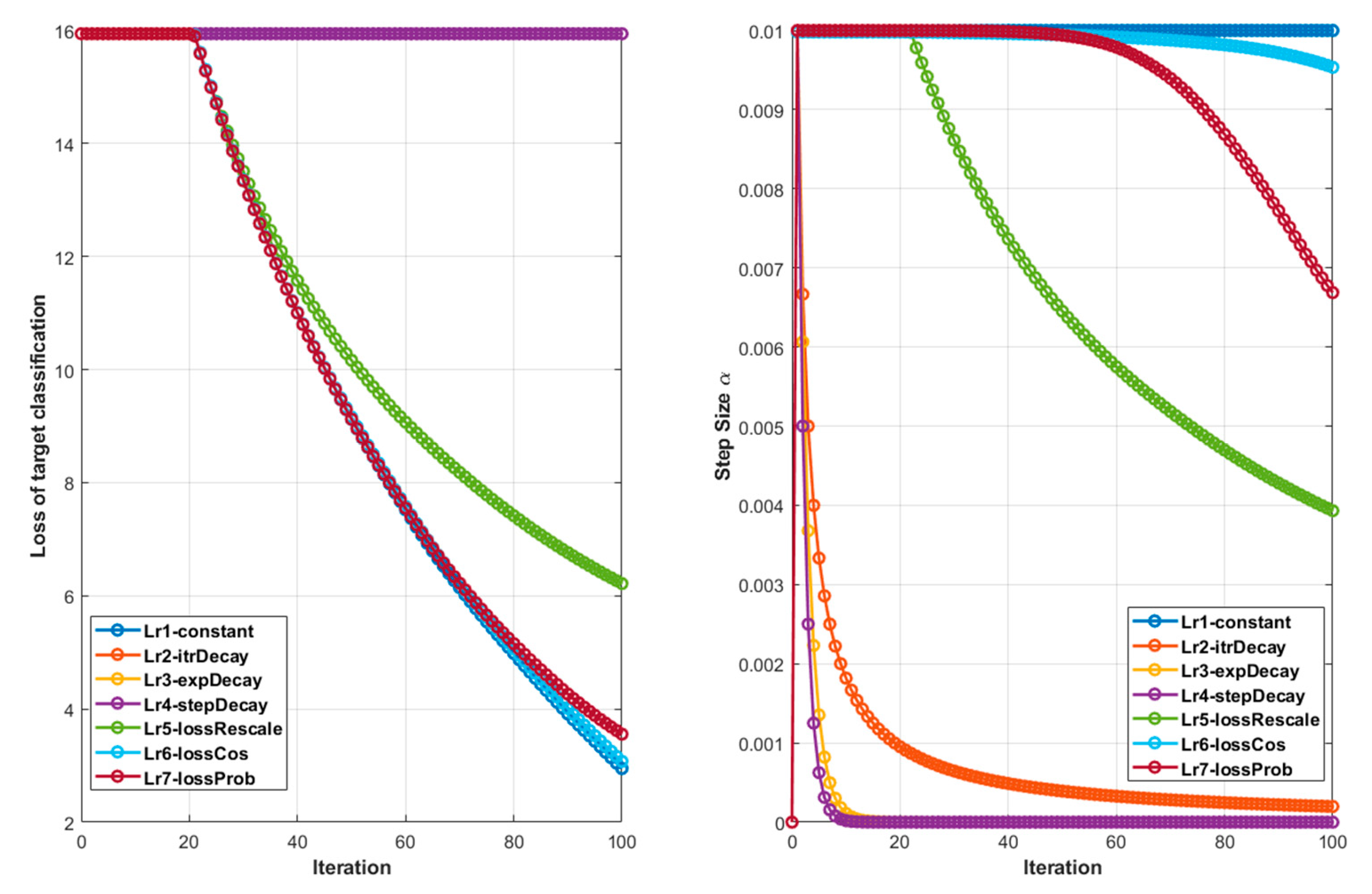
Trigonometric functions. The trigonometric function can rescale the loss vector without adding a prediction, as there is an angle ${\theta }_n$ at each iteration to measure the loss value (see Figure 3 for the loss axis).

Thus, when the target classification loss decreases in a target adversarial attack, the function is as follows:

$$F_n=\sin ({\tan }^{-1}\left(L_n\right))$$

(7)

When increasing the original classification loss in a non-target adversarial attack, the function is as follows:

$$F_n=\cos ({\tan }^{-1}\left(L_n\right))$$

(8)

3.

Directly apply the probability score of the original classification. It is an efficient and simple method to track the current loss status.

$$F_n=f_{\theta }\left(x, y_{origin}\right)$$

(9)

where $f_{\theta }\left(x\right)$ is the model prediction of $x$ and $f_{\theta }\left(x,y_{origin}\right)$ is the prediction probability for the original classification $y_{origin}$.

Additionally, the step size of the i-FGSM can be adjusted according to different decay functions [19]. There are very common learning rate decay algorithms found in the literature [25,26,27,28], such as iteration decay [29], exponential decay [30], and step decay [31]; hence, the total decay algorithms used in this paper are listed in

Table 2. The decay functions used in this paper. Where $\alpha ,{\alpha }_0,n$ represent the step size, initial step size, and iteration, respectively.

Index	Decay Algorithms	Formulars
1	Constant	$\alpha ={\alpha }_0$
2	Iteration decay	$\alpha ={\alpha }_0/\left(1+0.5\left(n-1\right)\right)$
3	Exponential decay	$\alpha ={\alpha }_0·e^{\left(-0.5\left(n-1\right)\right)}$
4	Step decay	$\alpha ={\alpha }_0·{0.5}^{floor\left(\left(n-1\right)/1\right)}$
5	Loss rescales	$\alpha ={\alpha }_0· \frac{L_n-L_{min}}{L_{max}-L_{min}} or {\alpha }_0·\left(1-\frac{L_n-L_{min}}{L_{max}-L_{min}}\right)$
6	Loss trigonometric	$\alpha ={\alpha }_0·\sin ({\tan }^{-1}\left(L_n\right)) or {\alpha }_0·\cos ({\tan }^{-1}\left(L_n\right))$
7	Loss probability	$\alpha ={\alpha }_0· f_{\theta }\left(x,y_{origin}\right)$

.

2.4. Evaluation Metric

The measurement of the shortest successful perturbation indicates which decay algorithm could effectively change the model prediction. To calculate the distance between the original image and the generated image, the L₂-norm function was applied. Usually, the distance of origin and adversary indicates the difficulty of changing the model prediction, and a larger distance corresponds to more robustness. I.e., in our experiment, the algorithm that generates a smaller perturbation to fool the model means that it is more effective at breaking through the model defense. It should be mentioned that some class samples are naturally far from the decision boundary influencing the required perturbation. Also, limitations of the optimization algorithm, i.e., the decay function, may complicate finding their adversary. To guarantee termination of the program, a limitation on the iterations was applied (see Algorithm 1). If the input image cannot be misclassified within 100 iterations, the algorithm fails to find its adversary. Thus, the success rate of finding an adversary is another evaluation metric to compare the algorithms.

To investigate the sensitivity of the algorithm to initial step size, three tests were run with the initial step size ${\alpha }_0$ set to 1, 0.1, or 0.01, respectively.

• The maximum iteration is 100. The iteration was stopped when the generated image was misclassified in case of the non-target attack or changed to the target class in case of the target attack. When the iteration exceeds 100, it is considered a failed case.
• The difference between the original image $x$ and the final generated adversarial image $x^{*}$ was calculated with $L_2$-norm distance [3,4,5], which is also defined by Euclidean distance, where $m$ is the number of pixels.

$$D\left(x,x^{*}\right)=||x^{*}-x{||}_2={\left({\sum }_{i=1}^m{\left|x^{*}-x\right|}^2\right)}^{\frac{1}{2}}$$

(10)

3.

There are also other common $L_p$-norm distance metrics, such as $L_0$ distance, $L_1$ distance, and $L_{\infty }$ distance [3,4,5], where $L_0$ distance measures the number of pixels that change in $x^{*}$ compare to image $x$; $L_1$ distance measures the sum of pixel distance that changes in $x^{*}$; and $L_{\infty }$ distance measures the maximum pixel change in $x^{*}$.

$$||x^{*}-x{||}_{\infty }=max\left(\left|x_1^{*}-x_1\right|,\dots ,\left|x_m^{*}-x_m\right|\right)$$

(11)

2.5. Adversary-Generating Algorithm

The whole adversary-generating program can be summed up in Algorithm 1.

Algorithm 1: Generate adversarial images with adaptive step size

Input: Trained model $f_{\theta }$, test sample set $\left\{x,y\right\}$, original class $y_{origin}$, target class $y_{target}$, the generated image and its classification at current iteration $\left\{x_n,y_n\right\}$, the probability score of the current input $x_n$ is $f_{\theta }\left(x_n\right)$, the cross-entropy loss at current iteration $L_n$, gradient sign map $S_g$, step size $\alpha$, the initial step size ${\alpha }_0$, iterations $n$, stopping criterion with maximum iteration limitation $n_{max}$. Output: The adversarial images around the classification boundary.

Part 1, Target Adversarial Attack: For $n$ < $n_{max}$:   If $y_n$ ~= $y_{target}$,   Calculate the current cross-entropy loss $L_n$ between the prediction $f_{\theta }\left(x_n\right)$ and $y_{target}$. Backpropagation through $f_{\theta }$ to get the gradient sign map $S_g$.   Loss adaptive decay algorithms:    1. Concatenate with the previous loss $\left\{L_1, L_2, \dots L_n,0\right\}$, rescale as the learning rate factor between [0, 1]: $\left\{F_1, F_2, \dots F_n,0\right\}$; $\alpha ={\alpha }_0 * F_n$;    2. $F_n=\sin ({\tan }^{-1}\left(L_n\right))$; $\alpha ={\alpha }_0 * F_n$;    3. $F_n=f_{\theta }\left(x, y_{origin}\right);$ $\alpha ={\alpha }_0 * F_n$;   Update $x_n$: $x_{n+1}=x_n-\alpha * S_g;$ $n=n+1;$   Elseif $y_n$ == $y_{target}$,   break; Part 2, Non-target Adversarial Attack: For $n$ < $n_{max}$:   If $y_n$ == $y_{origin}$, Calculate the current cross-entropy loss $L_n$ between the prediction $f_{\theta }\left(x_n\right)$ and $y_{origin}$. Backpropagation through $f_{\theta }$ to get the gradient sign map $S_g$.   Loss adaptive decay algorithms:    4. Concatenate with the previous loss $\left\{L_1, L_2, \dots L_n,L_n+1\right\},$ rescale as the learning rate factor between [0, 1]: $\left\{F_1, F_2, \dots F_n,1\right\}$; $\alpha ={\alpha }_0 * (1-F_n);$    5. $F_n=\cos ({\tan }^{-1}\left(L_n\right))$; $\alpha ={\alpha }_0 * F_n$;    6. $F_n=f_{\theta }\left(x, y_{origin}\right);$ $\alpha ={\alpha }_0 * F_n$;   Update $x_n$: $x_{n+1}=x_n+\alpha * S_g;$ $n=n+1;$   Elseif $y_n$ ~= $y_{origin}$,   break; Return: The generated image with minimal perturbations.

3. Results

As mentioned in the experimental settings, we use different decay functions to find adversaries. Each image has its unique ‘smallest perturbation’ within the experimental settings. To compare the efficiency of different decay functions, the mean smallest perturbation of all the successfully misclassified samples was calculated. In the target adversarial attack, the image is ‘perturbed’ in different directions according to the six different target classes. The weight space is sampled in those different directions (from the original class to a target classification boundary) by searching for the least perturbations.

Figure 4 depicts the success rate of finding adversaries using the target adversarial attack. When the initial step size is 1 (${\alpha }_0=1$), only the fourth function (step decay) and seventh function (using the original classification probability) failed to reach the target classification in 10 and 286 cases respectively; while there are 1400 samples times six target classes. In total, 8400 cases were presented in the target adversarial attack. When the step size is set to 0.1 and 0.01, as in the second function (iteration decay), third function (exponential decay), and fourth function (step decay), a clear drop in the success rate is found. A smaller initial step size and a rapid decline factor are slowing down the search process for the local minima, aggravating the negative impact on efficiency.

Figure 5 shows the shortest perturbation to find the target adversaries. The mean L₂-norm distances were calculated based only on the successfully generated adversaries. When the initial learning rate is 1 and 0.1, the first function (constant) and the sixth (loss trigonometric function) generated larger perturbations than others, and the fifth (loss rescale function) showed the fewest perturbations. When the initial learning rate is 0.01, the calculation was based only on thirty-seven joint successful cases, as the fourth (step decay) has a relatively low success rate to reach the target within 100 iterations. In this case, perturbations were approximately evenly distributed, indicating that the solution was strongly influenced by image properties (close to the classification boundary) rather than the decay algorithms.

In the non-target adversarial attack, the input image is automatically modified to the nearest adversarial classification region (see

Table 3. The nearest adversarial classification region when generating adversaries by the sixth (loss trigonometric function) in the non-target adversarial attack.

	Final Class with Maximum Percentage
Origin Class	${\mathit{\alpha }}_0=1$	${\mathit{\alpha }}_0=0.1$	${\mathit{\alpha }}_0=0.01$
1	7-(30.5%)	7-(30.5%)	7-(31.0%)
2	1-(60.5%)	1-(61.0%)	1-(60.5%)
3	1-(69.0%)	1-(64.5%)	1-(64.5%)
4	1-(42.0%)	1-(43.5%)	1-(44.0%)
5	1-(51.5%)	1-(46.0%)	1-(46.5%)
6	1-(45.0%)	1-(44.5%)	1-(43.5%)
7	1-(77.5%)	1-(78.5%)	1-(78.5%)

); thus, the distance should show the least perturbation compared to target adversaries. In total, there are 1400 cases in the non-target adversarial attack, and the success rate of finding adversaries shows similar results as in the target adversarial attack case.

When the initial step size is 1, in 100% of the cases, a misclassification is found, regardless of the used step size adaption. If the initial step size is 0.1 and 0.01, the success rate of the second, third, and fourth decay functions abruptly declines (see Figure 6).

The shortest perturbations are slightly different from the target adversarial attack. Figure 7 shows that the step decay function remains the smallest perturbation, regardless of the initial step size, and the first function (constant) remains the largest perturbation; our three loss-tracking functions generate fewer perturbations than the first function (constant) but more than the second, third, and fourth decay functions.

4. Discussion

According to the results, when the initial step size is 0.01, the difficulty increased to find an adversarial classification for the image samples, especially for the second iteration decay, third exponential decay, and fourth step decay functions. A ‘difficult’ image that failed to find its target adversary with all seven algorithms is shown in Figure 8. Although none of the decay functions could successfully find the target classification adversary, there are a few differences between them: the loss remains the same within 100 iterations when the step size uses the second, third, and fourth decay functions. Because the decayed step size drops down to nearly zero within ten iterations, these smaller and smaller step sizes stuck the algorithms for the local minima search; meanwhile, even with the constant function, the loss starts to move downward after twenty iterations. Compared with a rapidly decreased step size, the three loss-tracking functions are more stable. The loss rescale function has a similar trend with loss value, while the trigonometric function and loss probability are relatively slow to move downward; nevertheless, a more ‘flat’ step size gives these four functions (including the constant step size) the chance to find the final target classification after 100 iterations.

Another difficult image with a non-target adversary search presents the loss and step size slope in Figure 9. Similarly, the original classification loss remains unchanged when the step size decreases too fast (with the 2nd, 3rd, and 4th decay functions), while the original loss starts to increase after the 30th iteration with constant step size and loss-tracking functions. Compared to the target classification adversary search, the fifth (loss rescale function) generates a smaller step size and fewer perturbations (see Figure 5). In the non-target adversary search process, the seventh (original class probability) drops faster than the other two loss-tracking functions, generating relatively fewer perturbations (see Figure 7). For this reason, the trigonometric function has step size drops that are not as steep as other functions (see Figure 9), and it generated relatively higher perturbations.

Although using original classification probability to shorten the step size is efficient, there are drawbacks that question its reliability, especially in the target-class adversarial attack. Unlike the target classification loss value, which usually appears to be gradually decreasing in the target attack, the original probability does not always have a steadily decline, instead, sometimes it is shaped like a polyline or decreases suddenly when a third classification pops up in between the original and the target classification. Especially, when the initial step size is too large, increasing the risk of stepping into a wrong misclassification region (not the target classification), the step size goes down to nearly zero and thus cannot move forward to the target classification. For this reason, a larger initial step size would contrarily reduce the success rate (96.6%) when using the original classification probability to control the step size (see Figure 4).

The decay algorithms only affect the adversary that generated the use of more than one iteration. There are a number of cases that only rely on the initial step size when one iteration is sufficient to change the classification (see

Table 4. The number of cases that require only one iteration to find an adversary.

Decay Algorithms	Target Attack			Non-Target Attack
	${\mathit{\alpha }}_0=1$	${\mathit{\alpha }}_0=0.1$	${\mathit{\alpha }}_0=0.01$	${\mathit{\alpha }}_0=1$	${\mathit{\alpha }}_0=0.1$	${\mathit{\alpha }}_0=0.01$
1st Constant	2621	453	10	1050	317	9
2nd Iteration decay	2621	453	10	1050	317	9
3rd Exponential decay	2621	453	10	1050	317	9
4th Step decay	2621	453	10	1050	317	9
5th Loss rescales	2621	453	10	1050	317	9
6th Loss trigonometric	2617	447	10	1050	317	9
7th Loss probability	2608	434	6	1050	313	6

); therefore, finding the proper ‘initial step size’ is essential when searching for the minimal-distorted adversary.

In addition to setting a smaller initial step size, there are a few other transformations of the algorithms that could reduce the final perturbation; for instance, the modification can be restricted to half, a quarter, or other portions of the image, or to fewer pixels (see Figure 10). In this way, the quantified modification would be fewer than the way of evenly applying the perturbation on the whole image. For example, when we choose to modify half or a quarter of the image at each iteration, the L-norm distance is less than modifying the whole image; when the modification is applied on fewer pixels, the L-norm distance can be even less (see

Table 5. The different thresholds used to filter pixels with larger gradients affect the final perturbations that could change the model’s classification.

Threshold	Origin Class	Final Class	Iteration	L1-Norm	L2-Norm	Modify Portion
0	1	7	2	15.31 × 104	545.89	99.55%
1/2	1	4	2	6.70 × 104	270.15	49.30%
1/4	1	4	2	2.82 × 104	181.21	18.65%
Top 5000 pixel	1	4	3	1.25 × 104	127.61	7.71%
Top 500 pixel	1	4	12	5.00 × 103	119.13	2.04%
Top 100 pixel	1	7	55	4.08 × 103	158.33	1.18%

).

Additionally, there are some other limitations of the algorithm in finding the minimal-distorted adversary. In our experiment, the step-adaptive iterative fast gradient sign method (i-FGSM) was applied, accompanied by different kinds of decay functions. Therefore, at each iteration, the modification amplitude for all the pixels is the same, and only the modified directions are different based on the gradient sign. Additionally, our loss-tracking functions consider the ‘loss’ as a single variable that is independent from the cross-entropy loss function $J\left(\theta , x, y\right)$, thusthe predicted step size might lead the gradient search to a bad local minimum. Some other methods that could generate individual adaptive step sizes for every pixel would be helpful in finding a shorter adversarial perturbation. There are some high-dimensional step size adaptive methods proposed in machine learning [32], which can be implemented in the algorithm to precisely change the pixels. Anyway, the high-dimensional input space and high-dimensional parameter space of the CNN model still challenge the algorithm to find the global minimal perturbation to change an input image classification. As well as using Resnet-50 for image classification, this step-adaptive i-FGSM can be applied to different CNN model architectures.

5. Conclusions

In this research, we proposed the step-adaptive iterative fast gradient sign method to generate adversarial samples. The loss-tracking functions represent a relatively stable and shorter modification compared to the constant step size i-FGSM. Nevertheless, to generate more accurate and less-distorted adversaries, there are improvements possible that can be achieved by combining other search techniques. Adversarial training is a popular method to improve the CNN model robustness, but at the same time, if the generated adversarial samples for adversarial training are overmodified, they might reduce the model’s accuracy on legitimate images. In future work, in the context of adversarial training, this step-adaptive iterative fast gradient sign method can be used to generate adversarial images with the smallest perturbations while investigating the trade-off problem between robustness and accuracy.

References

- Twinanda, A.P.; Shehata, S.; Mutter, D.; Marescaux, J.; de Mathelin, M.; Padoy, N. Endonet: A deep architecture for recognition tasks on laparoscopic videos. IEEE Trans. Med. Imaging 2016, 36, 86–97. [Google Scholar] [CrossRef]
- Puttagunta, M.K.; Ravi, S.; Babu, C.N.K. Adversarial examples: Attacks and defences on medical deep learning systems. Multimed. Tools Appl. 2023, 82, 33773–33809. [Google Scholar] [CrossRef]
- Carlini, N.; Athalye, A.; Papernot, N.; Brendel, W.; Rauber, J.; Tsipras, D.; Goodfellow, I.; Madry, A.; Kurakin, A. On evaluating adversarial robustness. arXiv 2019, arXiv:1902.06705. [Google Scholar]
- Zhang, J.; Chen, L. Adversarial examples: Opportunities and challenges. IEEE Trans. Neural Netw. Learn. Syst. 2019, 31, 2578–2593. [Google Scholar] [CrossRef]
- Balda, E.R.; Behboodi, A.; Mathar, R. Adversarial examples in deep neural networks: An overview. In Deep Learning: Algorithms and Applications; Springer: Cham, Switzerland, 2020; pp. 31–65. [Google Scholar]
- Wiyatno, R.R.; Xu, A.; Dia, O.; De Berker, A. Adversarial examples in modern machine learning: A review. arXiv 2019, arXiv:1911.05268. [Google Scholar]
- Ding, N.; Möller, K. The Image flip effect on a CNN model classification. Proc. Autom. Med. Eng. 2023, 2, 755. [Google Scholar]
- Ren, K.; Zheng, T.; Qin, Z.; Liu, X. Adversarial attacks and defenses in deep learning. Engineering 2020, 6, 346–360. [Google Scholar] [CrossRef]
- Goodfellow, I.J.; Shlens, J.; Szegedy, C. Explaining and harnessing adversarial examples. arXiv 2014, arXiv:1412.6572. [Google Scholar]
- Kurakin, A.; Goodfellow, I.; Bengio, S. Adversarial machine learning at scale. arXiv 2016, arXiv:1611.01236. [Google Scholar]
- Dong, Y.; Liao, F.; Pang, T.; Su, H.; Zhu, J.; Hu, X.; Li, J. Boosting adversarial attacks with momentum. In Proceedings of the 2018 IEEE Conference on Computer Vision and Pattern Recognition, Salt Lake City, UT, USA, 18–23 June 2018. [Google Scholar]
- Madry, A.; Makelov, A.; Schmidt, L.; Tsipras, D.; Vladu, A. Towards deep learning models resistant to adversarial attacks. arXiv 2017, arXiv:1706.06083. [Google Scholar]
- Papernot, N.; McDaniel, P.; Jha, S.; Fredrikson, M.; Celik, Z.B.; Swami, A. The limitations of deep learning in adversarial settings. In Proceedings of the 2016 IEEE European Symposium on Security and Privacy (EuroS&P), Saarbrucken, Germany, 21–24 March 2016; IEEE: Piscataway, NJ, USA, 2016; pp. 372–387. [Google Scholar]
- Xiao, C.; Li, B.; Zhu, J.Y.; He, W.; Liu, M.; Song, D. Generating adversarial examples with adversarial networks. arXiv 2018, arXiv:1801.02610. [Google Scholar]
- Carlini, N.; Katz, G.; Barrett, C.; Dill, D.L. Provably minimally-distorted adversarial examples. arXiv 2017, arXiv:1709.10207. [Google Scholar]
- Croce, F.; Matthias, H. Minimally distorted adversarial examples with a fast adaptive boundary attack. In Proceedings of the 2020 International Conference on Machine Learning, PMLR, Virtual Event, 13–18 July 2020. [Google Scholar]
- Su, J.; Vargas, D.V.; Sakurai, K. One pixel attack for fooling deep neural networks. IEEE Trans. Evol. Comput. 2019, 23, 828–841. [Google Scholar] [CrossRef]
- Du, Z.; Liu, F.; Yan, X. Minimum adversarial examples. Entropy 2022, 24, 396. [Google Scholar] [CrossRef]
- Ding, N.; Möller, K. Using adaptive learning rate to generate adversarial images. Curr. Dir. Biomed. Eng. 2023, 9, 359–362. [Google Scholar] [CrossRef]
- Ding, N.; Möller, K. Robustness evaluation on different training state of a CNN model. Curr. Dir. Biomed. Eng. 2022, 8, 497–500. [Google Scholar] [CrossRef]
- Ding, N.; Möller, K. Generate adversarial images with gradient search. Proc. Autom. Med. Eng. 2023, 2, 754. [Google Scholar]
- Ding, N.; Arabian, H.; Möller, K. Feature space separation by conformity loss driven training of CNN. IFAC J. Syst. Control 2024, 28, 100260. [Google Scholar] [CrossRef]
- Gao, B.; Pavel, L. On the properties of the softmax function with application in game theory and reinforcement learning. arXiv 2017, arXiv:1704.00805. [Google Scholar]
- He, K.; Zhang, X.; Ren, S.; Sun, J. Deep Residual Learning for Image Recognition. arXiv 2015. [Google Scholar] [CrossRef]
- Learning Rate Schedules and Adaptive Learning Rate Methods for Deep Learning. 2017. Available online: https://towardsdatascience.com/learning-rate-schedules-and-adaptive-learning-rate-methods-for-deep-learning-2c8f433990d1 (accessed on 22 March 2017).
- Bengio, Y. Practical recommendations for gradient-based training of deep architectures. In Neural Networks: Tricks of the Trade, 2nd ed.; Springer: Berlin/Heidelberg, Germany, 2012; pp. 437–478. [Google Scholar]
- Bergstra, J.; Bengio, Y. Random search for hyper-parameter optimization. J. Mach. Learn. Res. 2012, 13, 281–305. [Google Scholar]
- Darken, C.; Moody, J. Note on learning rate schedules for stochastic optimization. In Proceedings of the Advances in Neural Information Processing Systems 3, Denver, CO, USA, 26–29 November 1990. [Google Scholar]
- Moreira, M.; Fiesler, E. Neural Networks with Adaptive Learning Rate and Momentum Terms; IDIAP: Martigny, Switzerland, 1995. [Google Scholar]
- Li, Z.; Arora, S. An exponential learning rate schedule for deep learning. arXiv 2019, arXiv:1910.07454. [Google Scholar]
- Ge, R.; Kakade, S.M.; Kidambi, R.; Netrapalli, P. The step decay schedule: A near optimal, geometrically decaying learning rate procedure for least squares. In Proceedings of the Advances in Neural Information Processing Systems 32, Vancouver, BC, Canada, 8–14 December 2019. [Google Scholar]
- Ruder, S. An overview of gradient descent optimization algorithms. arXiv 2016, arXiv:1609.04747. [Google Scholar]