Abstract
Innovative wood inspection technology is crucial in various industries, especially for determining wood quality by counting rings in each stave, a key factor in wine barrel production. (1) Background: Traditionally, human inspectors visually evaluate staves, compensating for natural variations and characteristics like dirt and saw-induced aberrations. These variations pose significant challenges for automatic inspection systems. Several techniques using classical image processing and deep learning have been developed to detect tree-ring boundaries, but they often struggle with woods exhibiting heterogeneity and texture irregularities. (2) Methods: This study proposes a hybrid approach combining classical computer vision techniques for preprocessing with deep learning algorithms for classification, designed for continuous automated processing. To enhance performance and accuracy, we employ a data augmentation strategy using cropping techniques to address intra-class variability in individual staves. (3) Results: Our approach significantly improves accuracy and reliability in classifying wood with irregular textures and heterogeneity. The use of explainable AI and model calibration offers a deeper understanding of the model’s decision-making process, ensuring robustness and transparency, and setting confidence thresholds for outputs. (4) Conclusions: The proposed system enhances the performance of automatic wood inspection technologies, providing a robust solution for industries requiring precise wood quality assessment, particularly in wine barrel production.
1. Introduction
The visual grading of wood surfaces is a challenging task due to the combination of strict grading rules, significant natural variations in the material, and the subjectivity of appearance criteria, making it difficult to accurately assess each defect type, size, and location. The oak used to make barrels for the aging of wines and spirits is classified according to its origin and grain type [1]. Visual grading is the primary method used to assess the tightness of wood grain, which is determined by the average distance between annual growth rings. A growth ring represents the yearly increase in a tree’s circumference or width from early spring to winter. Older trees exhibit slower growth rates than younger trees, and trees grown in cooler climates tend to have tighter grains than those grown in warmer climates. The tightness of the grain in an oak barrel significantly impacts the aroma and tannin levels of wine. Finer grain releases more aromatic compounds, while coarser grain contributes to higher tannin levels [2]. The classification criteria for staves can differ from one manufacturer to another, as they may use various types of wood and have distinct standards. Nevertheless, as per the information provided by our client for this particular project, the staves were categorized into the following three distinct groups based on the number of growth rings per inch: extra-fine grain, fine grain, and coarse grain. It is important to note that the specific range for each classification is determined by the individual manufacturer and the type of wood they are working with, reflecting a tailored approach to barrel making.
The classification of wood is frequently performed by trained human experts. This procedure is time-consuming, expensive, and laborious [3]. Manual inspection depends on field circumstances, labor perception, and performance, which are connected to factors like weariness, tension, and motivation [4]. As a result of these issues, it is imperative to develop an automated method for assessing the quality of products; computer vision offers the best solution to this problem.
A variety of computer vision techniques can be used for classification. Because different species of wood have such a wide range of features, more sophisticated systems can completely replace the human factor, greatly increasing company profits. However, the error rate and reliability of different methods also tend to vary [5].
In the wood processing industry, most visual quality inspections are still performed by knowledgeable human operators. Visual inspection is a difficult, monotonous activity with a significant chance of human error. Automatic systems for wood imaging processing have been developed, mainly focusing on species classification, defect and knot detection, and ring identification.
Kwon et al. [6] proposed a convolutional neural network with a LeNet-modified architecture to classify Korean wood species using cropped images, achieving 99.3% accuracy among five categories. Using microscopic images, Zhu et al. [7] trained an improved Faster RCNN model to classify 10 types of wood and to locate the main characteristics of each type of wood, achieving 83.8% accuracy. An exhaustive comparison was carried out by de Geus et al. [8] between a pre-designed classical feature method and deep learning models, obtaining much better results with the latter approach in classifying 11 different wood species, with a final accuracy of 98.13%.
Regarding the detection and classification of defects, Niskanen et al. [9] implemented an unsupervised self-organized map to detect knots and anomalies for wood inspection, achieving a detection accuracy of 96%. Urbonas et al. [10] used data augmentation and a Faster RCNN to identify defects in wood veneer surfaces, achieving 96.1% accuracy. He et al. [11] developed an original DCNN architecture to locate and classify defects; they used dropout, L2 regularization, and data augmentation to avoid the overfitting problem, obtaining an accuracy of 99.13%.
There are fewer solutions concerning ring detection, and those that have been developed use homogeneous images without large variations or noise. DeepDendro is the first approach using convolutional neural networks to perform automatic ring segmentation; it was presented by Fabijanska and Danek [12] and uses a U-Net-based architecture to extract rings from clean and homogeneous images of wood surfaces with 97% precision. As can be seen in Figure 1, the images used in this research are of staves without imperfections, in which grains (rings) can be clearly observed.
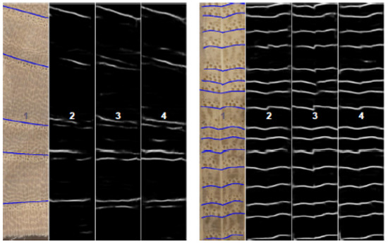
Figure 1.
Staves used in DeepDendro research [12].
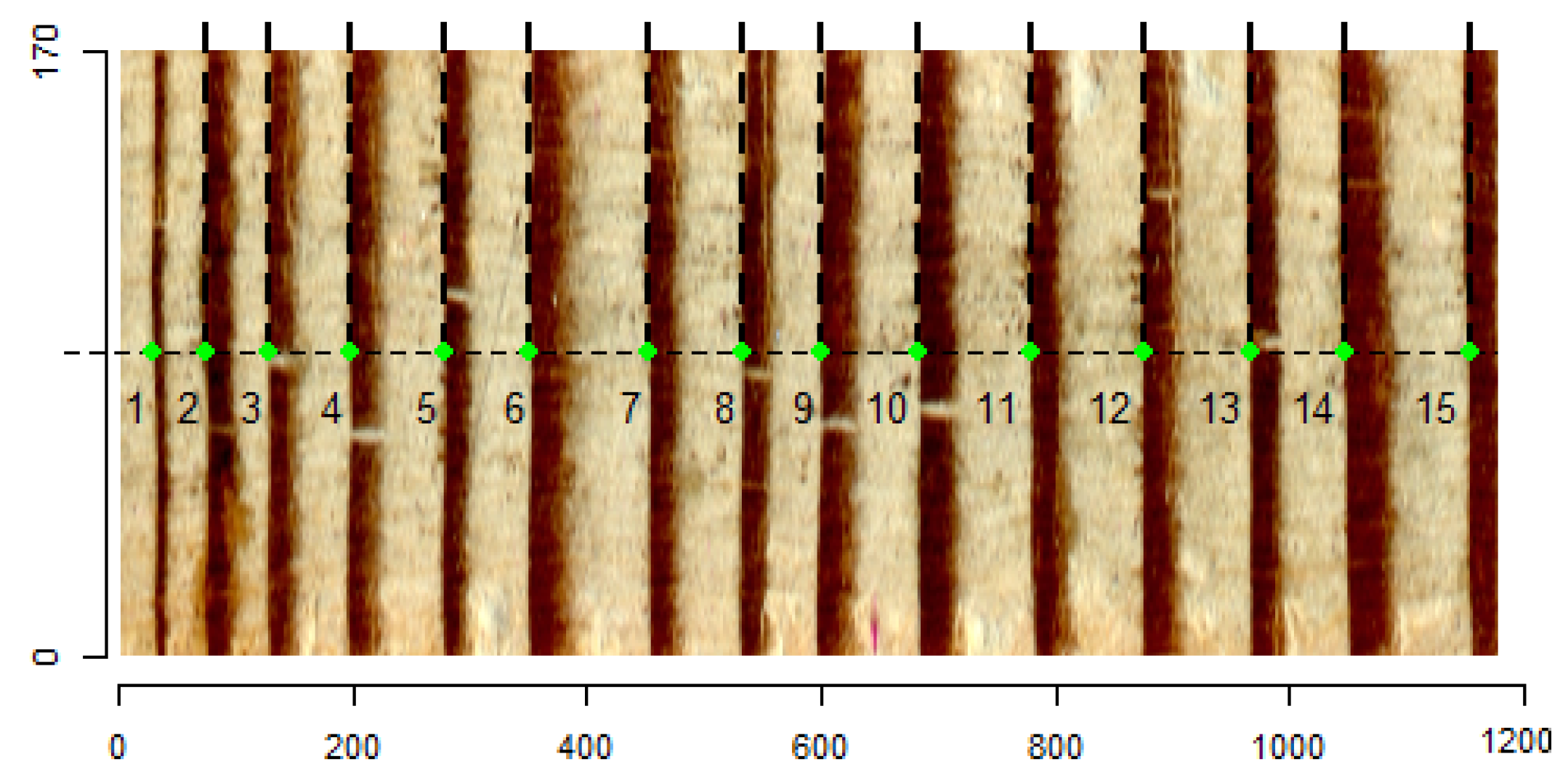
MtreeRing is an R package for the automatic measurement of tree-ring widths that uses classical processing techniques like morphological filters, the Canny edge detector, and linear algorithms on homogeneous images with well-defined and straight rings; it was developed by Shi et al. [13], achieving a correct detection average of 92.45%. Similar to DeepDendro, in the images used in this research, the rings are easily distinguishable, as shown Figure 2 (green dots).

Figure 2.
Staves used in MteeeRing research [13].
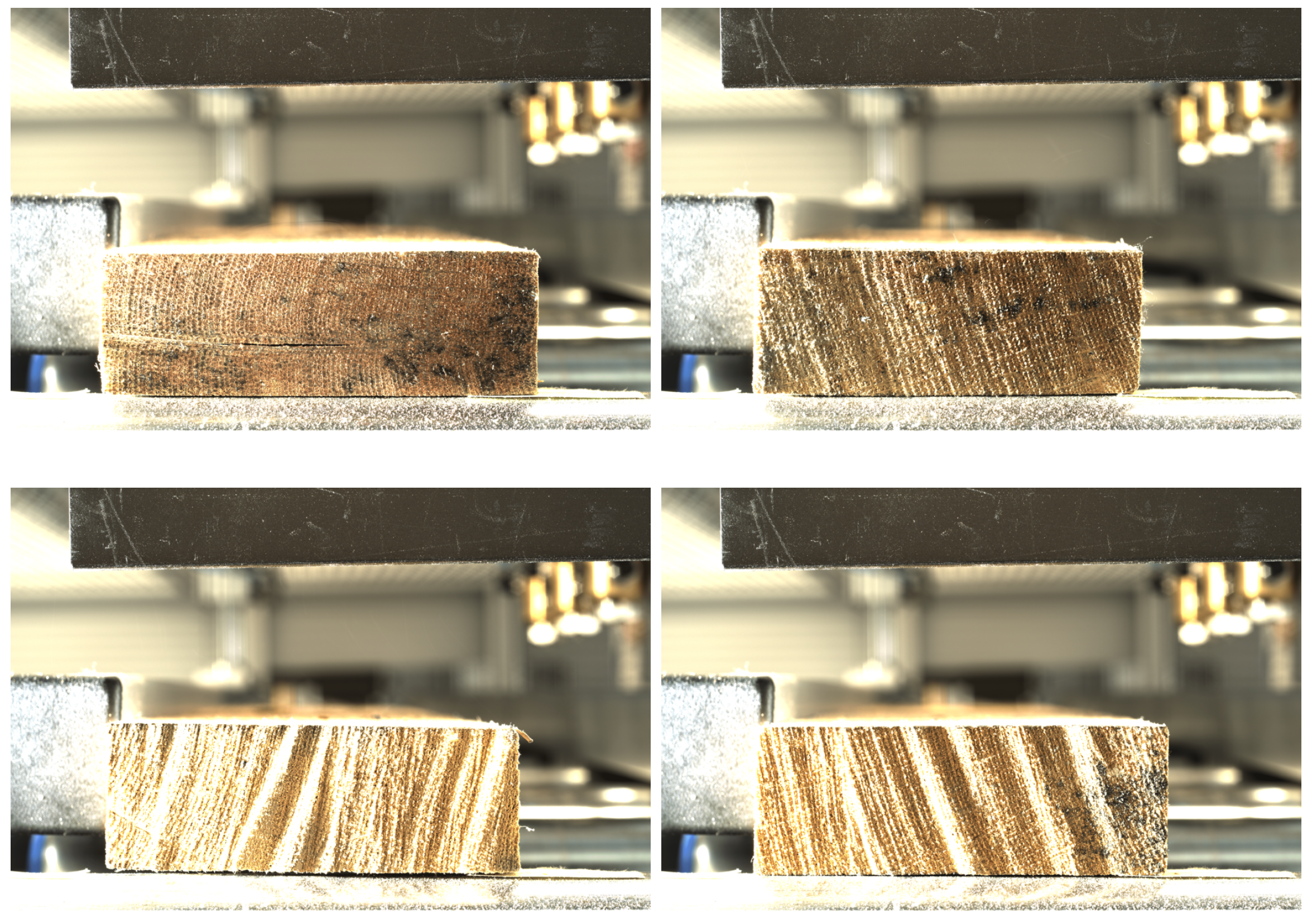
In summary, there are already several works on direct wood classification and/or ring segmentation, but all of them use clean samples where the rings or defects are clearly visible. Our work proposes an approach applied after sawing that deals with very heterogeneous, irregular, and dirty samples, which often contain texture defects that could confuse the algorithm, as shown in Figure 3.
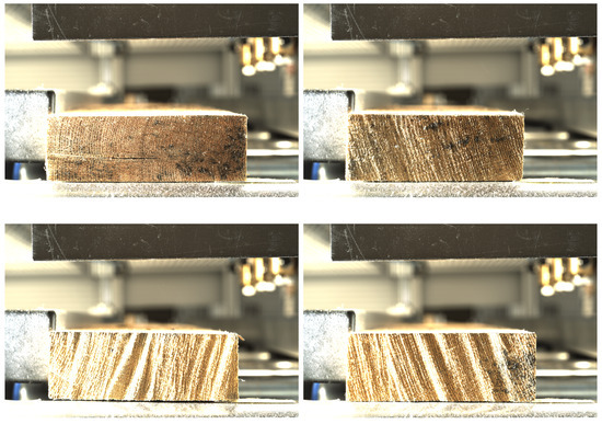
Figure 3.
Different examples of staves after sawing, showing the heterogeneity.
Our solution is designed to be implemented on a machine that processes staves during the production of wine barrels, ensuring accurate classification despite these difficult conditions. The main contributions of this work are outlined as follows:
- We create an image database of staves for wine barrel production. The database contains 1805 images of complete staves and 4238 manually labeled cropped images (1.3 cm2) of the staves. The database is available upon reasonable request.
- We develop a preprocessing pipeline using classical techniques to remove background noise and enhance the most important features, followed by classification with a deep learning model cropped images of wine barrel staves with noticeable heterogeneity, achieving high precision and low execution time.
- We design a system that can be implemented in an automated machine that processes staves continuously. The entire process, from image acquisition to stave grading, takes fewer than 2 s.
2. Data Acquisition and Preprocessing
2.1. Optical Setup and Development Environment
The camera used in this study was an IDS U3-3800CP-C-HQ with a 1″ sensor size, 20 Mpx resolution (5536 × 3692), and a 25 mm focal-length lens. The staves were illuminated laterally with diffuse light from an Effilux EFF-SMART-06-000. This directional light highlights perpendicular defects, such as vertically oriented rings. The use of diffuse light reduces shadows and reflections, providing more uniform illumination and enhancing the visibility of surface details [14].
The preprocessing algorithms were developed in house in C# programming language using Visual Studio 2019, incorporating the Halcon 22 integration libraries is a robust software solution for machine vision that offers a complete set of features and functionalities, along with an integrated development environment. C# was used to develop the user interface for a better touch and feel, as this software was integrated in the machine in charge of positioning the staves and launching the trigger for image acquisition.
Python is a powerful language for developing and training deep learning models, but it is relatively slow and has high energy consumption [15,16]. For these reasons, Python was used for training the deep learning algorithms, and the final model was converted to ONNX format [17] for use in the C# application to achieve better execution time and efficiency.
2.2. Image Filtering with Classic Techniques
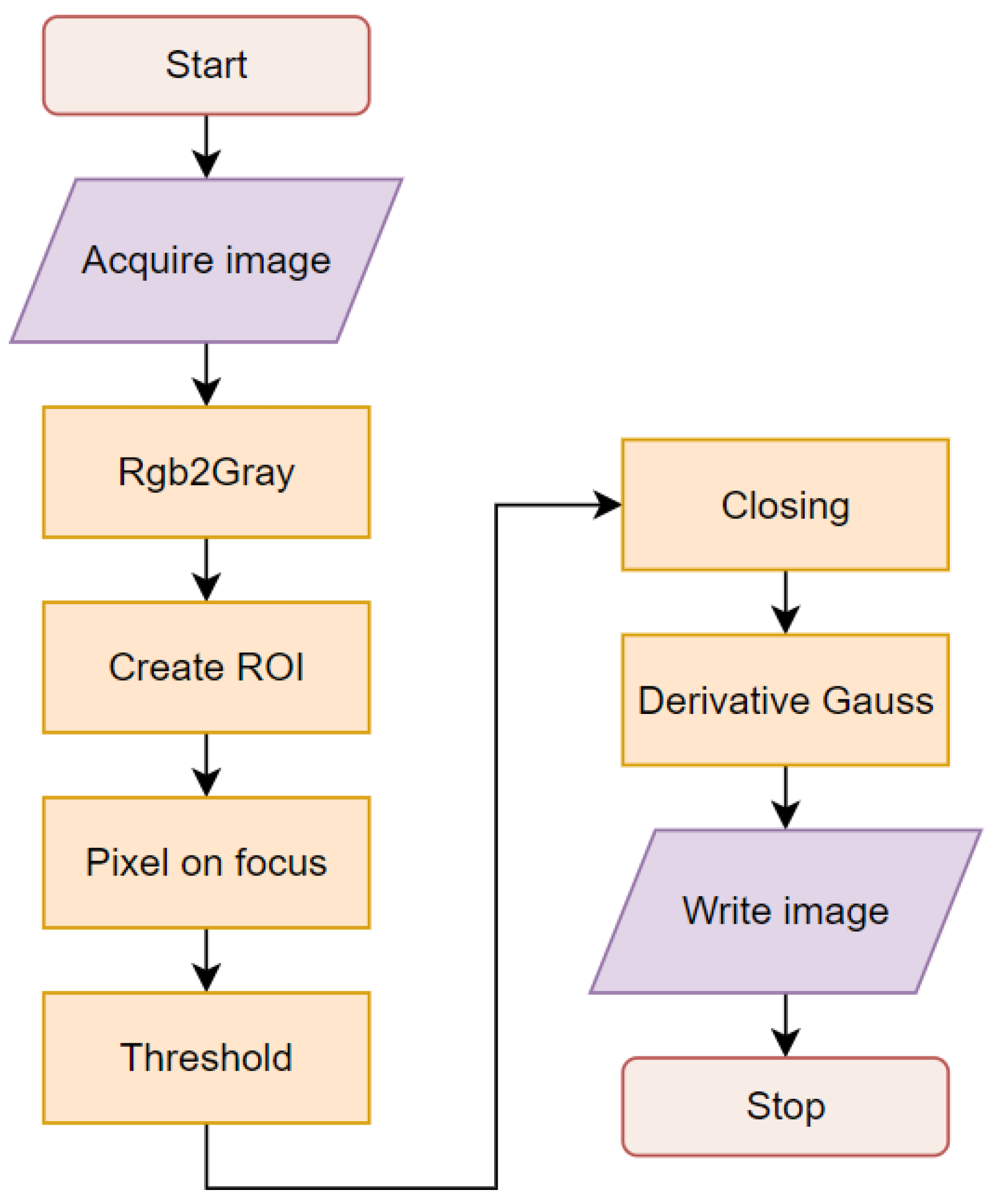
Images of wood staves after sawing show noticeable heterogeneity in their characteristics; for that reason, it is necessary to preprocess the images to enhance the most important features and eliminate the background and shapes that do not provide information about grain density. Image processing starts with the camera acquiring the image, and several algorithmic steps are used for filtering, thresholding, segmentation, and detection. Figure 4 shows a block diagram of the algorithms used in this study.
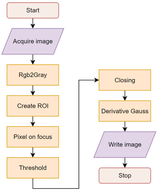
Figure 4.
Algorithm for preprocessing.
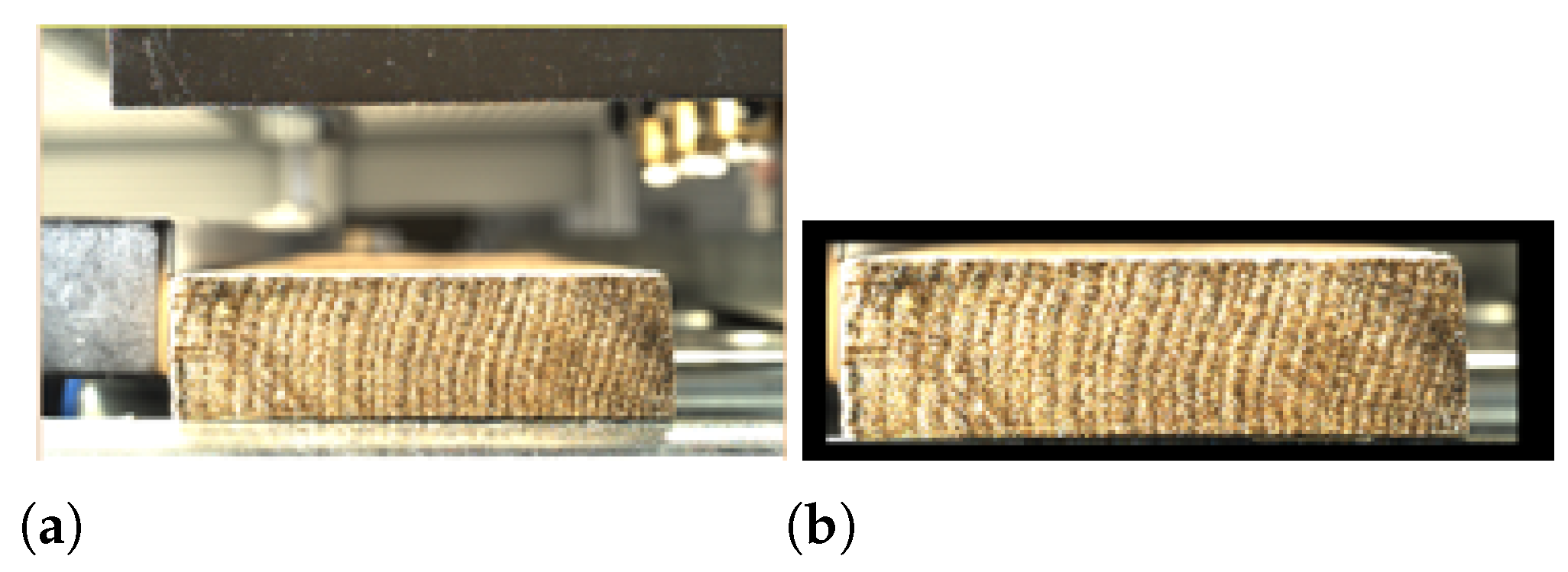
Knowing the maximum and minimum stav dimensions, a region of interest (ROI) of the image can be selected with sufficient confidence, as shown in Figure 5.
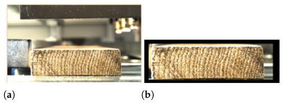
Figure 5.
Input image (a) and region of interest (b).
As the optical setup is designed to focus on the staves, the background of the image is out of focus. To select only the stave, a pixel-on-focus algorithm was developed. The criteria for quantifying the focus of an image are usually based on the evaluation of the image’s sharpness by looking at the gradient function [18]. To perform the operation, the image is converted to grayscale because the colors are not particularly important to this application and it is less computationally intensive to process a grayscale image than an RGB image. The analysis is performed according to Equation (1). Additionally, a threshold operator is used to select the pixels whose gray values (g) fulfill the condition shown in Equation (2). The result of the process is shown in Figure 6.

Figure 6.
Image after application of the pixel-on-focus algorithm (a) and after the threshold (b).
To eliminate internal holes and noisy edges, morphological dilation and erosion filters are applied to the resulting image. Morphological dilation makes objects more visible and fills in small holes in objects. On the other hand, morphological erosion removes floating pixels, and shapes appear smaller [19]. Applying erosion after dilation keeps the original region shape dimensions while closing internal holes and removing external noise. The operator that joins the two filters is called the closing operator. It is described in Equation (3), and the result is shown in Figure 7.

Figure 7.
Morphological filters: (a) dilation; (b) closing = dilation + erosion.
The result of the morphological filters is the exact region in which the stave is located. In the last step, to highlight the pixels where high-intensity changes occur (rings), a Sobel filter is applied. This filter is a convolution with the derivative of the Gaussian (on the x axis to highlight vertical lines), as expressed in Equation (4). The derivative works very well to highlight edges, and a Gaussian is applied in order to smooth the result and remove noise [20]. The result of this high-pass filter is shown in Figure 8.

Figure 8.
Input image (a) and result of the Sobel filter (b).
Finally, Figure 9 shows a comparison of an original image captured by the camera with the final image after all preprocessing. The background is removed, and the grains (rings) of the stave are highlighted.

Figure 9.
Input image (a) and final result (b).
3. Crop Classification Using Deep Learning
3.1. First Classification Approach
The first approach involves the use of MVTec’s Deep Learning tool from Halcon [21]. Using the “Enhanced” model of the library, a good accuracy value of 95.77% was obtained on the test data; however, the model performed poorly when tested on new data. In response to this problem, the heat maps provided by the program itself were analyzed, revealing that the model was not being activated in the pixels where the rings were located; instead, it exhibited almost random activation, as can be seen in Figure 10.

Figure 10.
Heat maps of the first approach.
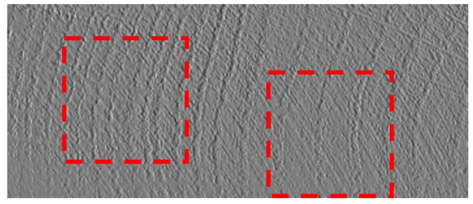
The model performed well with the initial type of wood, but its effectiveness decreased when wood from different forests became available. Analyzing the images, in addition to the natural variations in the staves, intra-class problems were frequently observed. Some areas had many rings, while others had few, as shown in Figure 11. Therefore, we decided to implement a custom deep learning model to process an image as a collection of crops, as training an algorithm with complete stave images would be inaccurate.
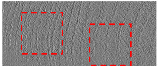
Figure 11.
Intra-class problem: red box on the left contains 8 rings, red box on the right contains 3.
3.2. Crops/Data Augmentation and Labeling
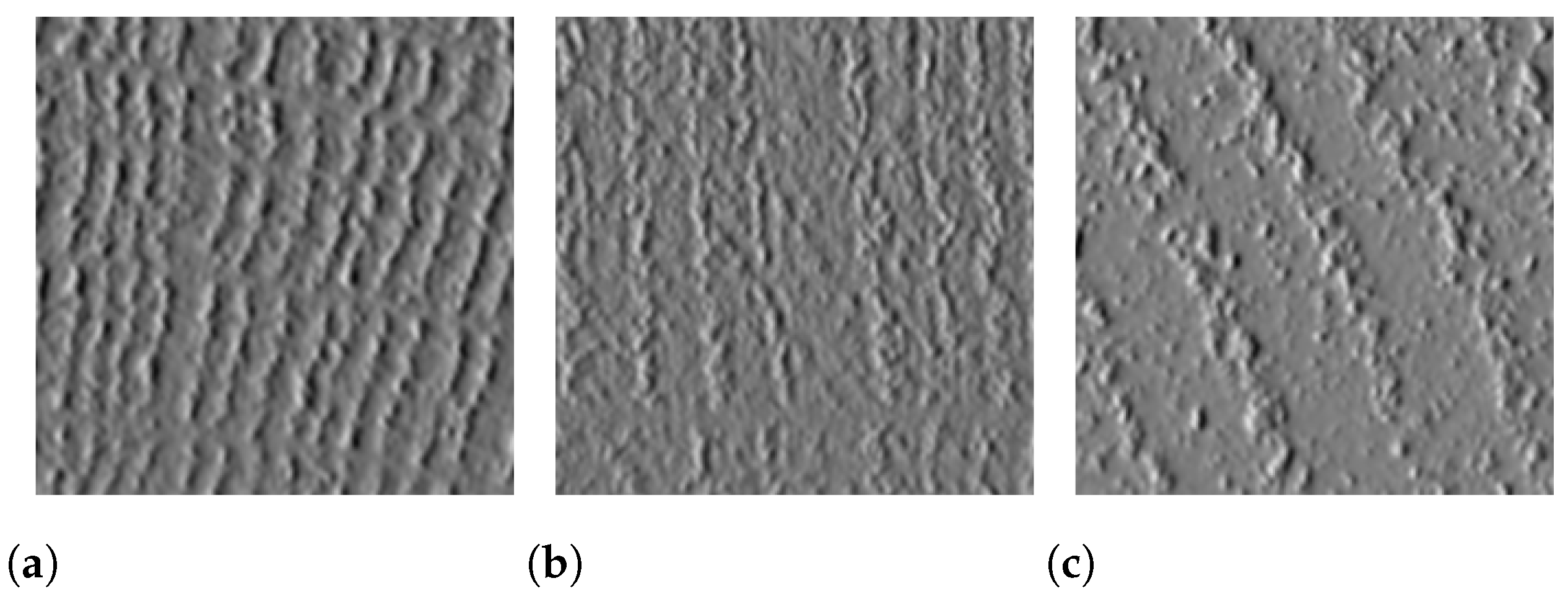
To solve the intra-class problem, a cropping approach was developed. From the initial set of 180 received images of staves, 1.3-square-centimeter crops were randomly selected. Later, additional images of staves arrived; however, no crops were extracted from these. As a result, only 10% of the total images were used for crop creation. The number of visually distinguishable rings was counted to classify each crop according to this number (labeling step). The crop set for each class was created using the customer’s proposed grading range of extra fine to fine and coarse, as described in Table 1 and shown in Figure 12.

Table 1.
Range of stave classification.
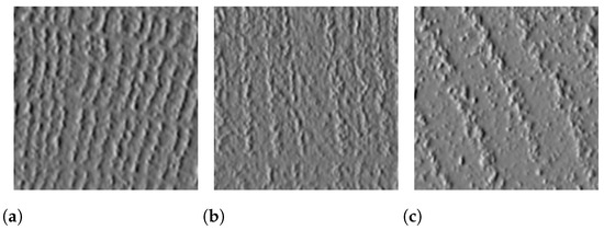
Figure 12.
Created crops: (a) extra fine; (b) fine; (c) coarse.
It is important to mention that only crops with distinguishable and well-defined rings were included in the image database. As can be seen in the table above, there is a significant imbalance in the extra-fine class due to the limited number of images available of this type of stave. For this reason, data augmentation techniques needed to be implemented to ensure balanced datasets.
Data augmentation (DA) is a method that generates additional training examples by manipulating existing samples. It is a cost-effective and efficient technique for enhancing the performance and accuracy of machine learning models, particularly in scenarios where data availability is limited [22]. Existing training samples can be reused as fresh data by incorporating noise, altering color settings, and adding other effects like blur and sharpening filters. In our work, to achieve class balance, vertical/horizontal flips and brightness adjustments were applied to crops of the extra-fine class. The final number of crops is shown in Table 2, and Figure 13 describes the augmentation process.

Table 2.
Total crops after augmentation.
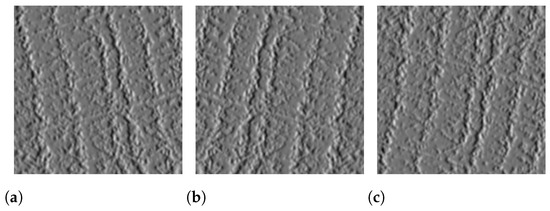
Figure 13.
Input image (a) and results using transformations of horizontal flip (b) and vertical flip (c).
The crops were divided into training, validation, and test sets, using those generated with data augmentation only for training. The number of images was distributed as shown in Table 3.

Table 3.
Set distribution.
3.3. Used Architectures
There is no script or pattern for selecting a convolutional neural network architecture, and there is always the possibility that the same or better results can be obtained by using another one. In our case, first tests were performed with several known architectures, and the best results in terms of accuracy were obtained with neural network models based on ResNet and the EfficientNet family. It is important to note that the final model must not only be accurate but also fast, since it will be implemented in a machine that processes staves continuously. In this regard, members of the EfficientNet family are among the fastest known methods to date [23].
ResNet is a deep neural network architecture that was first introduced in 2015 by researchers from Microsoft [24]. It is known for its ability to train very deep neural networks with as many as hundreds of layers while avoiding the problem of vanishing gradients. The vanishing gradient problem occurs when the gradients in the early layers of a deep neural network become very small during training, making it difficult to update the weights and improve the network’s performance. ResNet has been used with great success in a variety of applications, including image recognition, object detection, and natural language processing.
EfficientNet is a family of neural network architectures introduced in 2019 by researchers from Google [23]. These architectures are designed to be highly efficient in terms of computational resources while achieving state-of-the-art performance on image classification tasks. The main idea behind EfficientNet is to use a compound scaling method that uniformly scales the depth, width, and resolution of the network.
Apart from the backbone architecture (ResNet or EfficientNet), we added three dense layers in order to improve the training, which we classified into three categories, as well as dropout units, to avoid possible overfitting. The proposed architecture can be observed in Figure 14.
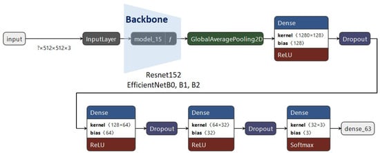
Figure 14.
The proposed architecture.
3.4. Training Strategies and Results
Training was performed with different configurations, each of which (starting from the second one) responded to results obtained in previous studies. The functions and hyperparameters of all stages are detailed in Table 4. It is important to note that the “class weights” parameter was used to force the network to give more importance to the classification of the fine class, which was the worst performer in the first stage. To increase the accuracy of the models, parts of their convolutional layers were also declared trainable. Data augmentation was implemented at run time to address the persistent challenge of overfitting, a problem that remained unresolved in the initial four stages of the model training process. This led to a model that performed exceptionally on the training set but poorly on the validation and test sets. To mitigate this issue, data augmentation plays a crucial role by artificially increasing the diversity of the training dataset.

Table 4.
Training stages.
The best results after training were obtained with the ResNet152V2-based model and the EfficientNet B1-based model, as can be see in Table 5. Considering the requirement of speed in inference, it was decided to go for the second one and continue with it for other training stages in search of better results.

Table 5.
Crop accuracy by stage.
Overfitting was the main problem encountered in the previous stages of training, even with increases in the number of training images and large variations that were applied to the images with increasing runtime data augmentation. This represents a fundamental problem in supervised machine learning that prevents the generalization of models to fit both the data observed in the training set and the unobserved data in the test set. To mitigate its impact, in addition to the existing measures that were implemented, it is suggested in the literature to incorporate weight regularization in the network. This approach aims to ensure that models perform well in addressing real-world challenges by selecting relevant features and distinguishing between more and less useful ones [25].
L2 regularization is one of the most used techniques in this regard. Its application consists of adding a regularizing term determined by a regularization factor () to the cost function and multiplying by the square of the weights, as shown in Equation (5) for the case of the categorical cross-entropy used in our project [26].
In optimizers with adaptive gradient algorithms, such as the Adam optimizer used in this project, L2 regularization does not bring the expected improvement. Therefore, we implemented the strategy known as weight decay, which has been proven to substantially improve the generalization of models by extracting the regularization factor from the cost function and applying a similar one in the optimizer, as shown in Equation (6) [26].
where w represents weights, is LR, is the first term (momentum), is the second term, is the coefficient, and represents regularization.
Applying weight decay to the optimizer, increasing the number of trainable layers of the model, and adjusting the parameters for runtime data augmentation as shown in Table 6, two other training stages were implemented, obtaining better results, as shown in Table 7.

Table 6.
EfficientNet B1 tuning.

Table 7.
Crop accuracy.
3.5. Saliency Maps and Grad-CAM Analysis
In recent years, Explainable AI (XAI) techniques have gained popularity as a research focus in the field. This is due to the difficulty in comprehending and trusting the outcomes of many AI models, which are often considered black boxes. XAI methods aim to enhance trust in the decision making of these models [27]. To evaluate our model results, saliency maps and Grad-CAM algorithms were implemented. The analysis was motivated by the results obtained using the first approach, as shown in Figure 10.
Saliency maps represent a visualization technique used to help understand which parts of an input image are most important for the output produced by a neural network. The output of a linear model is computable as proposed in Equation (7), where I is the input image, is the class score, and and are the weight vector and bias of the model, respectively. Mathematically, the magnitude of the elements in defines the importance of each pixel in I to the class score () [28].
Although CNNs are complex nonlinear models, they can be approximated with a linear function in the neighborhood of the input image using a first-order Taylor expansion, where corresponds to the first derivative gradient of the network output with respect to the input image. Therefore, as shown in Equation (8), the values of the gradients define the importance of the pixels of I in the output of the network [28].
The Gradient-weighted Class Activation Maps (Grad-CAMs) generate a visual explanation from CNNs without requiring architectural changes. In this technique, the gradient of an output () is computed with respect to the feature maps of a convolutional layer (A). These gradients are global average-pooled (Equation (9)). The result is used to weigh the feature maps, which, after a ReLU activation (Equation (10)), produce a heat map that shows which regions of the image were most important for the model’s decision [29].
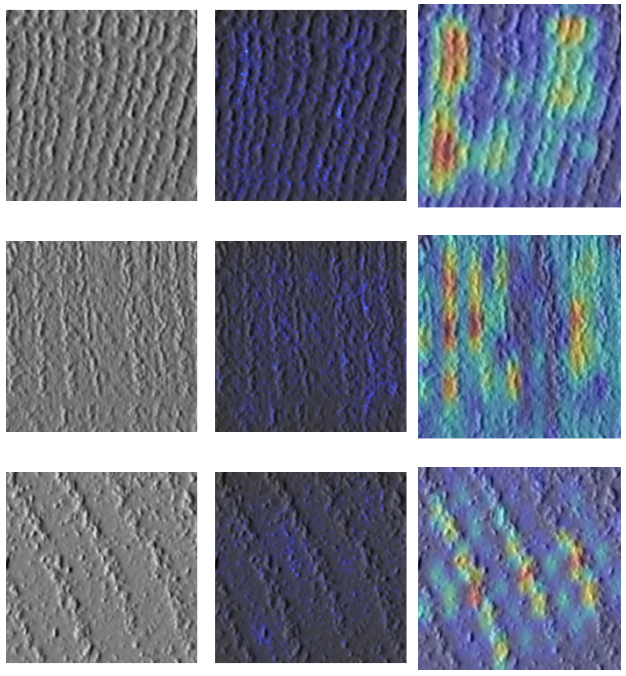
Figure 15 shows the results of the application of these methods to crops of each of the classes. For the case of saliency maps, it can be observed that activation increases with an increase in the number of rings in the images, indicating that the model output correlates with the number of rings. The Grad-CAMs also show that the most important feature maps for the classification of the model are those where the rings are found, as these areas are particularly activated. Despite not explicitly instructing the network on what to focus on, the results of XAI techniques show that the model is, indeed, paying attention to what is considered important, i.e., the number of rings.
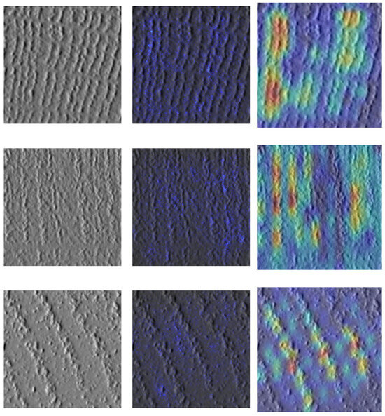
Figure 15.
Inputs (left), saliency maps (center), and Grad-CAMs (right).
3.6. Model Calibration Analysis
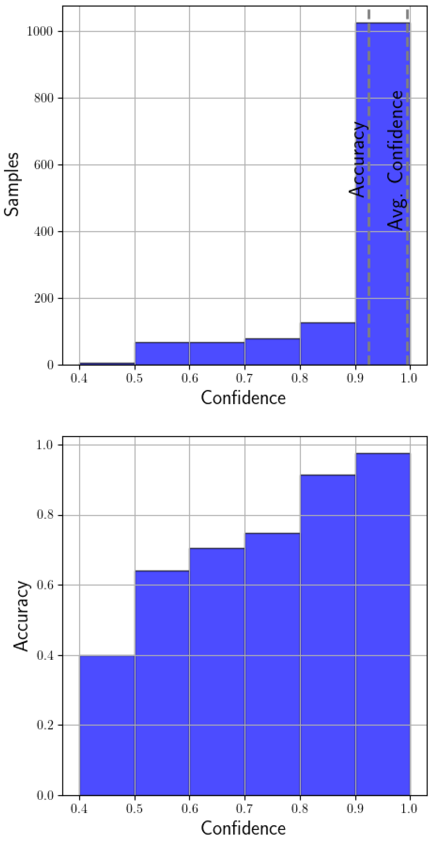
Once the obtained model classified crops with a 0.92 accuracy, it was decided to analyze whether the model was calibrated. A model is defined as calibrated when the confidence of occurrence of a class corresponds to the accuracy for that confidence [30]. Perfect calibration is described in Equation (11), where the probability that a prediction () belongs to class given the confidence of the prediction p is p. In this sense, a perfectly calibrated model should have a mean confidence equal to the accuracy of the model. With a miscalibrated model, high confidences could have lower accuracies, which is critical in a variety of applications [30].
Reliability diagrams are a visual representation of model calibration. The diagrams plot accuracy as a function of the confidence of the prediction. If the model is perfectly calibrated, the plot should correspond to the identity function [31]. As can be seen in the top of Figure 16, the confidences that occur the most are between 0.9 and 1.0, and with an accuracy of 0.92, the model is not perfectly calibrated but is very close to being so. The bottom of the figure shows, for example, that the model has an accuracy of 0.91 for predictions with confidences between 0.8 and 0.9 and over 0.97 for predictions with confidences grater than 0.9. For this reason, the model is very reliable for predictions with confidences higher than 0.8.

Figure 16.
Model calibration histograms.
4. Stave Classification Based on Crops
4.1. Strategies for Crop Selection
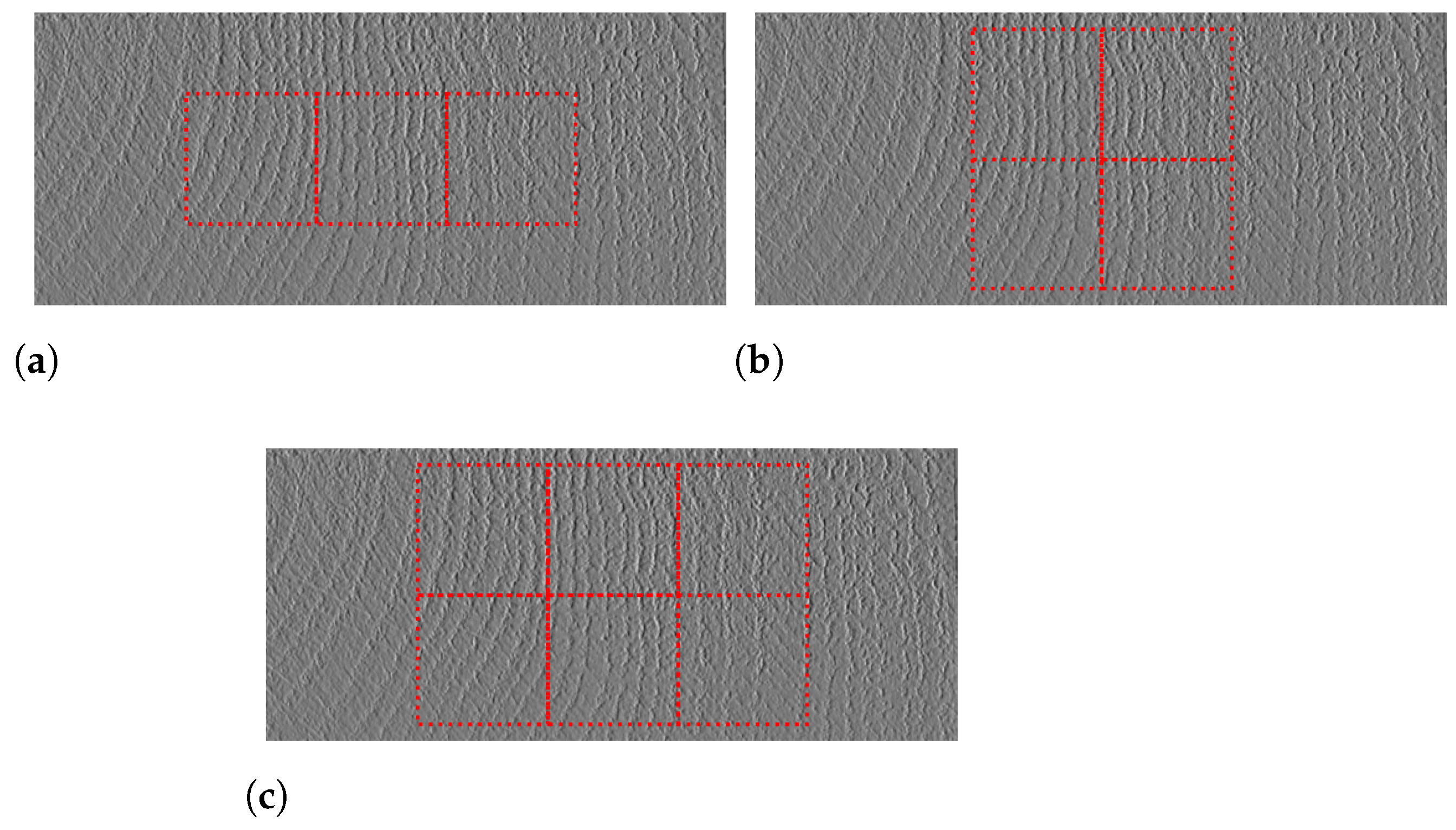
Once a deep learning model has been obtained, it is necessary to develop strategies for the selection of crops to be classified in the staves. The customer indicates, as a reference, that the classification should consider, above all, the central part of the stave, since the edges are processed in later stages of the operation. Based on this guideline, the crops selection strategies shown in Figure 17 were implemented. The number of staves used to test the model is shown in Table 8.
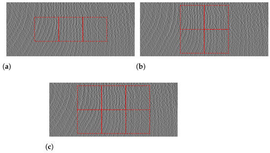
Figure 17.
Crop selection strategies: (a) 3 central crops; (b) 4 central crops; (c) 6 central crops.

Table 8.
Total staves.
4.2. Voting System Design and Results
Based on the three cropping strategies described above, a first processing of the complete staves was performed, determining the stave class with the greatest presence among the crops. The disadvantage of this solution is that no processing is performed in cases of ties, where the output is prioritized from extra fine to coarse. In this analysis, the classification threshold of the model was varied from 0.5 to 0.8, as shown Table 9. As seen in Section 3.6, the model achieved an accuracy of greater than 0.91 for thresholds higher than 0.8.

Table 9.
Sum of crop classification.
A second solution was developed to overcome the drawback of the first voting system. In this case, the class of the stave is determined as the class that has the highest cumulative probability from the sum of the probabilities of each crop. The results are shown in Table 10.

Table 10.
Sum of probability classification.
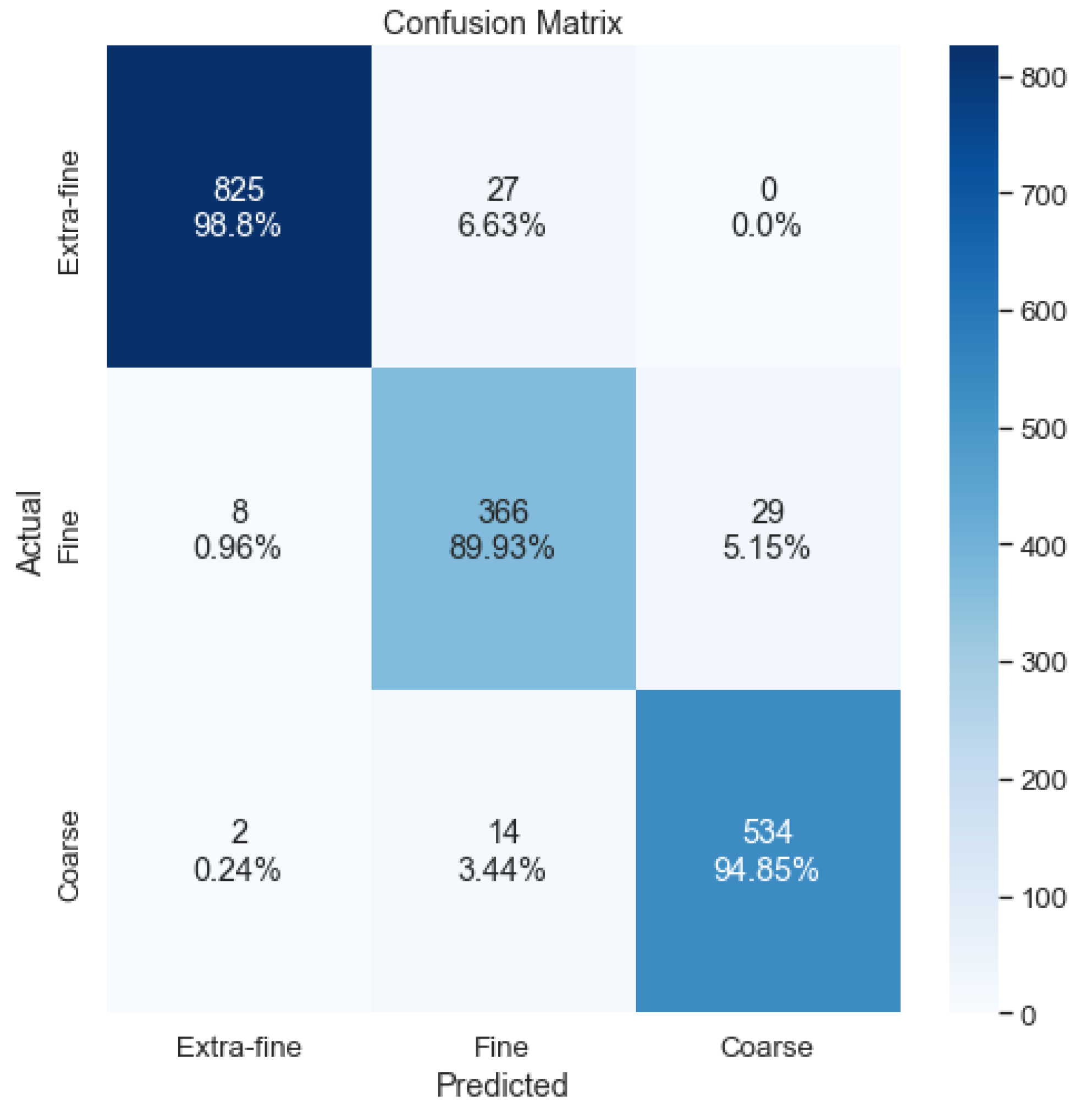
Considering only the accuracy, the first solution (6 crops), with a threshold of 0.8, is that which offers the best results. To perform the analysis of the errors made by the model, a confusion matrix was obtained, as shown in Figure 18. It can be seen that there are errors that are considered serious, as two coarse staves are classified as extra fine. This error is considered to be related to staves with few or no classified crops due to the threshold value of 0.8, since in the case of a tie between extra fine and coarse, the output is extra fine.

Figure 18.
Sum of the crop confusion matrix.
A hybrid voting system is then proposed, combining the number of crops in each class and the cumulative probability. In cases of ties in terms of the highest number of crops or in cases in which no crop exceeds the threshold, the output is the class that has the highest cumulative probability in the sum of all crops. A formal explanation is shown in Equation (12). As can be seen in Table 11, the accuracy of this voting system is not better than that the first proposed system; however, we proceed to analyze the errors made with the confusion matrix shown in Figure 19.

Table 11.
Hybrid classification.

Figure 19.
Confusion matrix of the hybrid system.
With the hybrid voting method, no serious errors are made, since no cross-classifications between the extra-fine and coarse classes are seen in the confusion matrix. For this reason, despite achieving slightly lower accuracy than the first method, we decided to use this method for the final output of the stave classification system. A summary of the crop classification strategies and their results is shown in Table 12.

Table 12.
Summary of strategies.
The execution time recorded during the tests, with the machine in operation–from image capture through to the classical preprocessing stage, the classification of the six central crops, and the final decision by the voting system–, was approximately s per stave.
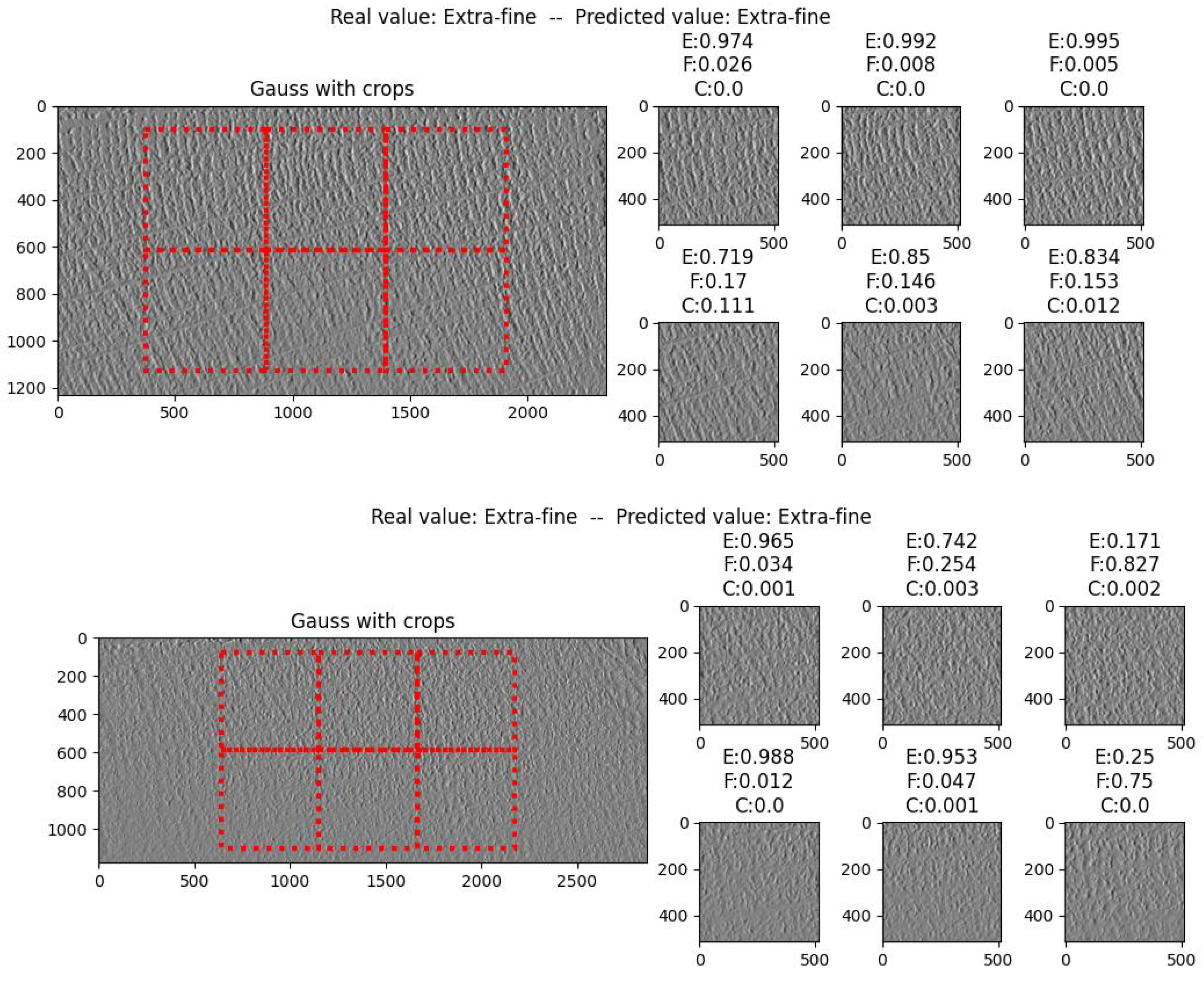
Once the final model for stave classification was obtained, we decided to compare its results with those obtained with MtreeRing to verify if MtreeRing is capable of detecting the grains (rings). As can be observed in Figure 20, in both cases, there are several rings—and even sections of rings—that are not detected. This is to be expected because, as mentioned above, the package was designed to work with homogeneous images with clearly distinguishable rings. In contrast, the obtained model correctly classifies the selected images, as shown in Figure 21.

Figure 20.
Results of the MtreeRing package on selected images.
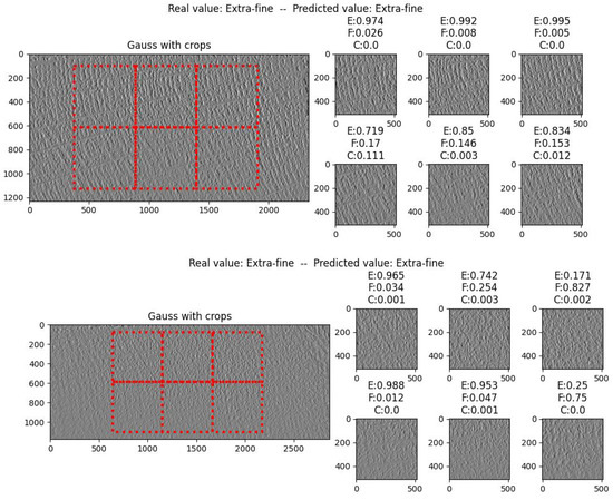
Figure 21.
Results using the obtained model on selected images.
5. Conclusions
This paper addresses the challenge of wood quality classification in staves, which exhibit significant heterogeneity and irregularity due to natural conditions and sawing effects. To the best of our knowledge, this work represents the first intelligent system for grain classification in the production of wine barrels. Our approach integrates classical computer vision techniques with deep convolutional neural networks to preprocess images, highlighting ring boundaries and subsequently classifying staves based on the number of rings.
A significant contribution of this study is the creation of an extensive image database specifically for wine barrel staves, comprising 1805 images of complete staves and 4238 manually labeled crops (1.3 cm²). This database, which available upon reasonable request, serves as a foundational resource for further research and development in this field. Moreover, the system was designed for future implementation in automated machinery capable of processing staves continuously. The entire process, from image acquisition to stave grading, is completed in less than 2 s, demonstrating the system’s suitability for industrial applications.
Additionally, to demonstrate the robustness, transparency, and confidentiality of the model, we applied explainable AI (XAI) techniques and analyzed model calibration to ensure that the model’s confidence in predictions was consistent with its accuracy. The final solution is a fast and accurate system for classifying staves after the sawing process.
In future work, the implementation of an artificial intelligence algorithm to replace the current voting system represents a promising avenue for further research. This approach has the potential to enhance classification results by identifying patterns in the arrangement of crops within the stave. To optimize the performance of this algorithm, it will be necessary to gather a larger dataset than is presently available. This dataset should be constructed such that the independent variables are the probabilities assigned by the model to each crop within the stave, while the dependent variable corresponds to the class of the stave.
Author Contributions
F.A.R.: writing—original draft, software, validation, formal analysis, visualization, and investigation; M.E.: software and data curation; D.K.M.: investigation and conceptualization; D.B.: conceptualization, methodology, validation, resources, writing—review and editing, supervision, and project administration. All authors have read and agreed to the published version of the manuscript.
Funding
This work was supported by REEPRODUCE project, funded by the European Union Grant Agreement N° 101057733.
Data Availability Statement
Data will be made available upon reasonable request.
Conflicts of Interest
The authors declare no conflicts of interest.
References
- Sánchez-Gómez, R.; del Alamo-Sanza, M.; Nevares, I. Volatile composition of oak wood from different customised oxygenation wine barrels: Effect on red wine. Food Chem. 2020, 329, 127181. [Google Scholar] [CrossRef] [PubMed]
- Botezatu, A.; Essary, A. A Guide to Traditional Oak Barrels; Technical Report; The Texas A & M University System: College Station, TX, USA, 2020. [Google Scholar]
- Sun, P. Wood quality defect detection based on deep learning and multicriteria framework. Math. Probl. Eng. 2022, 4878090. [Google Scholar] [CrossRef]
- Kolus, A.; Wells, R.; Neumann, P. Production quality and human factors engineering: A systematic review and theoretical framework. Appl. Ergon. 2018, 73, 55–89. [Google Scholar] [CrossRef] [PubMed]
- Nurthohari, Z.; Murti, M.; Setianingsih, C. Wood quality classification based on texture and fiber pattern recognition using hog feature and svm classifier. In Proceedings of the IEEE International Conference on Internet of Things and Intelligence System, Bali, Indonesia, 5–7 November 2019; pp. 123–128. [Google Scholar] [CrossRef]
- Kwon, O.; Lee, H.; Lee, M.; Jang, S.; Yang, S.; Park, S.; Choi, I.; Yeo, H. Automatic wood species identification of Korean softwood based on convolutional neural networks. J. Korean Wood Sci. Technol. 2017, 45, 797–808. [Google Scholar] [CrossRef]
- Zhu, M.; Wang, J.; Wang, A.; Ren, H.; Emam, M. Multi-fusion approach for wood microscopic images identification based on deep transfer learning. Appl. Sci. 2021, 11, 7639. [Google Scholar] [CrossRef]
- de Geus, A.; Backes, A.; Gontijo, A.; Albuquerque, G.; Souza, J. Amazon wood species classification: A comparison between deep learning and pre-designed features. Wood Sci. Technol. 2021, 55, 857–872. [Google Scholar] [CrossRef]
- Niskanen, M.; Silvén, O.; Kauppinen, H. Wood inspection with non-supervised clustering. Mach. Vis. Appl. 2003, 13, 275–285. [Google Scholar] [CrossRef]
- Urbonas, A.; Raudonis, V.; Maskeliūnas, R.; Damaševičius, R. Automated identification of wood veneer surface defects using faster region-based convolutional neural network with data augmentation and transfer learning. Appl. Sci. 2019, 9, 4898. [Google Scholar] [CrossRef]
- He, T.; Liu, Y.; Yu, Y.; Zhao, Q.; Hu, Z. Application of deep convolutional neural network on feature extraction and detection of wood defects. Measurement 2020, 152, 107357. [Google Scholar] [CrossRef]
- Fabijańska, A.; Danek, M. DeepDendro—A tree rings detector based on a deep convolutional neural network. Comput. Electron. Agric. 2018, 150, 353–363. [Google Scholar] [CrossRef]
- Shi, J.; Xiang, W.; Liu, Q.; Shah, S. MtreeRing: An R package with graphical user interface for automatic measurement of tree ring widths using image processing techniques. Dendrochronologia 2019, 58, 125644. [Google Scholar] [CrossRef]
- Martin, D. A practical guide to machine vision lighting. Adv. Illum. 2007, 2007, 1–3. [Google Scholar]
- Olivari, L.; Olivari, L. Influence of Programming Language on the Execution Time of Ant Colony Optimization Algorithm. Teh. Glas. 2022, 16, 231–239. [Google Scholar] [CrossRef]
- Gordillo, A.; Calero, C.; Moraga, M.Á.; García, F.; Fernandes, J.P.; Abreu, R.; Saraiva, J. Programming languages ranking based on energy measurements. Softw. Qual. J. 2024. [Google Scholar] [CrossRef]
- ONNX. ONNX: Open Neural Network Exchange, Version 1.16.1; Linux Foundation: San Francisco, CA, USA, 2024.
- Moru, D.; Borro, D. Analysis of different parameters of influence in industrial cameras calibration processes. Measurement 2021, 171, 108750. [Google Scholar] [CrossRef]
- Gonzalez, R.; Woods, R. Digital Image Processing; Pearson: London, UK, 2018. [Google Scholar]
- Forsyth, D.; Ponce, J. Computer Vision: A Modern Approach; Pearson: London, UK, 2012. [Google Scholar]
- GmbH, M.S. HALCON—The Powerful Software for Your Machine Vision Application. Version 22. 2024. Available online: https://www.mvtec.com/products/halcon (accessed on 22 October 2024).
- Wong, S.; Gatt, A.; Stamatescu, V.; McDonnell, M. Understanding Data Augmentation for Classification: When to Warp? In Proceedings of the International Conference on Digital Image Computing: Techniques and Applications, Gold Coast, Australia, 30 November–2 December 2016; pp. 1–6. [Google Scholar] [CrossRef]
- Tan, M.; Le, Q. Efficientnet: Rethinking model scaling for convolutional neural networks. In International Conference on Machine Learning; PMLR: New York, NY, USA, 2019. [Google Scholar] [CrossRef]
- He, K.; Zhang, X.; Ren, S.; Sun, J. Deep Residual Learning for Image Recognition. In Proceedings of the IEEE Conference on Computer Vision and Pattern Recognition, Las Vegas, NV, USA, 27–30 June 2016; pp. 770–778. [Google Scholar] [CrossRef]
- Ying, X. An Overview of Overfitting and its Solutions. J. Phys. Conf. Ser. 2019, 1168, 022022. [Google Scholar] [CrossRef]
- Loshchilov, I.; Hutter, F. Decoupled weight decay regularization. arXiv 2017. [Google Scholar] [CrossRef]
- Ali, S.; Abuhmed, T.; El-Sappagh, S.; Muhammad, K.; Alonso-Moral, J.; Confalonieri, R.; Guidotti, R.; Ser, J.; Díaz-Rodríguez, N.; Herrera, F. Explainable artificial intelligence (xAI): What we know and what is left to attain trustworthy artificial intelligence. Inf. Fusion 2023, 99, 101805. [Google Scholar] [CrossRef]
- Simonyan, K.; Vedaldi, A.; Zisserman, A. Deep inside convolutional networks: Visualising image classification models and saliency maps. In Proceedings of the Workshop at International Conference on Learning Representations, Banff, AB, Canada, 14–16 April 2014. [Google Scholar] [CrossRef]
- Selvaraju, R.; Das, A.; Vedantam, R.; Cogswell, M.; Parikh, D.; Batra, D. Grad-CAM: Visual Explanations from Deep Networks via Gradient-Based Localization. In Proceedings of the IEEE International Conference on Computer Vision, Venice, Italy, 22–29 October 2017; pp. 618–626. [Google Scholar] [CrossRef]
- Guo, C.; Pleiss, G.; Sun, Y.; Weinberger, K.Q. On calibration of modern neural networks. In Proceedings of the International Conference on Machine Learning, Sydney, Australia, 6–11 August 2017; pp. 1321–1330. [Google Scholar] [CrossRef]
- Niculescu-Mizil, A.; Caruana, R. Predicting good probabilities with supervised learning. In Proceedings of the 22nd International Conference on Machine Learning, Bonn, Germany, 7–11 August 2005; pp. 625–632. [Google Scholar] [CrossRef]
Disclaimer/Publisher’s Note: The statements, opinions and data contained in all publications are solely those of the individual author(s) and contributor(s) and not of MDPI and/or the editor(s). MDPI and/or the editor(s) disclaim responsibility for any injury to people or property resulting from any ideas, methods, instructions or products referred to in the content. |
© 2024 by the authors. Licensee MDPI, Basel, Switzerland. This article is an open access article distributed under the terms and conditions of the Creative Commons Attribution (CC BY) license (https://creativecommons.org/licenses/by/4.0/).


