Abstract
Purpose: The impact of hybrid quantum-classical neural network (NN) architectures with multiple backbones and quantum transformation as a data augmentation (DA) technique on image classification tasks was investigated using the CIFAR-10 and MedMNIST (DermaMNIST) datasets. These datasets were chosen for their relevance in general-purpose and medical-specific small-scale image classification, respectively. Methods: A series of quanvolutional transformations, utilizing random quantum circuits based on single-qubit rotation quantum gates (Y-axis, X-axis, and combined XY-axis transformations), were applied to create multiple quantum channels (QC) for input augmentation. By integrating these QCs with baseline convolutional NN architectures (LCNet050) and scalable hybrid NN architectures with multiple (n) backbones and separate QC (n) inputs (HNN-QCn), the scalability and performance enhancements offered by quantum-inspired data augmentation were evaluated. The proposed cross-validation workflow ensured reproducibility and systematic performance evaluation of hybrid models by mean and standard deviation values of metrics (such as accuracy and area under the curve (AUC) for the receiver operating characteristic). Results: The results demonstrated consistent performance improvements by AUC and accuracy in HNN-QCn models with the number n (where ) of backbones and QC inputs across both datasets. The different improvement rates were observed for the smaller increase in AUC and the larger increase in accuracy as input complexity (number of backbones and QCs inputs) increases. It is assumed that the prediction probability distribution is becoming sharpened with the addition of backbones and QC inputs, leading to larger improvements in accuracy. At the same time, AUC reflects these changes more slowly unless the model’s ranking ability improves substantially. Conclusion: The findings highlight the scalability, robustness, and adaptability of HNN-QCn architectures, with superior performance by AUC (micro and macro) and accuracy across diverse datasets and potential for applications in high-stakes domains like medical imaging. These results underscore the utility of quantum transformations as a form of DA, paving the way for further exploration into the scalability and efficiency of hybrid architectures in complex datasets and real-world scenarios.
1. Introduction
Image classification is a fundamental topic of research in computer vision and Artificial Intelligence (AI) domains. It has far-reaching implications in many practical and scientific fields. Industries that highly benefit from recent advancements in image classification algorithms and approaches range from such important and practical domains as healthcare, automotive and content moderation platforms to miscellaneous fields of cutting-edge scientific research such as self-driving cars or satellite imagery analysis. Modern advanced image classification algorithms are used for classifying increasingly complex images and are applied to datasets exponentially increasing in size. This comes down to the fact that modern image classification algorithms often require intensive computations and extensive dataset sizes for model training, which translates to high operational and infrastructure costs for systems that require the utilization of advanced image classification models. This problem is one of the driving forces behind the research that explores alternative paradigms.
Quantum computing is one of the promising alternative computing paradigms that have the potential to revolutionize the vast majority of domains including AI. By utilizing such principles of quantum mechanics as entanglement and superposition of quantum particles, quantum computing offers the promise of exponential speed-up of operations. Quantum Machine Learning (QML) and Quantum Deep Learning (QDL) emerged as novel fields of research that focus on utilizing quantum computing to improve the efficiency of computations for different fields of AI, including image classification. The recent extensive review of the advancements in QML and QDL that focused on the image classification problem [1,2,3] emphasized the limitations and challenges of existing approaches and drafted gaps in the field.
Quantum computing is based on the concept of qubit (quantum bit). Qubit is a fundamental unit of quantum information, which is an analog to a bit in classical computing. The key feature of a qubit is the ability to exist in a state of superposition. There are various technologies for creating qubits. One of the most used types of physical qubits is superconductor qubits, which use superconducting materials and require ultra-low temperatures for maintaining coherence [4]. Another widely used type of qubit is trapped ion qubits, which use ions trapped in electromagnetic fields and are manipulated using lasers [5]. There are also other prominent technologies for creating qubits that are not as widely used currently as the aforementioned, but they still can be promising and fruitful in the future, such as creating spin-based qubits based on coupled quantum dots [6].
Recent research in the QML field indicated that Hybrid Neural Networks (HNNs) can be a very promising approach that allows for the integration of quantum hardware into classical neural networks. One such prominent research was undertaken by Henderson et al. [7], who proposed an algorithm of utilizing a quantum device as a quantum convolutional layer followed by a number of classical neural network layers and thus forming “Quanvolutional” NN (QNN), which expands the possibilities of QML.
Another promising area of the novel research field is quantum-inspired algorithms. Some of the recent research in this area indicates that quantum computing can be used to enhance image classification operations and address the increasing resource demands imposed by increasing the complexity level of machine learning problems [8]. A new QNN architecture was proposed that offers improvements in the data encoding process, and faster convergence and higher accuracy were achieved on MNIST and MNIST-Fashion datasets.
Recently, various advanced QNN architectures showed improvements on various pattern recognition problems over classical architectures by leveraging principles of quantum computing [9,10,11,12], various classic NN [13] and quantum-classic [14] hybridization schemes. This indicates that HNNs and QNNs are very promising domains of research that can benefit various practical fields and industries.
This paper’s aim is to comprehensively evaluate how various factors impact the performance of hybrid neural networks (HNNs), focusing on enhancing their capabilities through several advancements. Specifically, the study explores the following aspects:
- Broadening the types of quantum transformations under investigation by incorporating a wider range of quantum operations on their contribution to input data representation within the HNN framework;
- Expanding HNN by increasing the number of QC input data channels and integrating multiple backbone (MB) architectures;
- Integrating and adopting other classical NN architectures, such as LCNet, to serve as baselines or components of hybrid models that could allow for direct performance comparison between purely classical, hybrid, and quantum-enhanced networks.
This approach examines how additional data channels and parallel processing pipelines can enhance feature diversity and improve the model’s performance across different standard (like general-purpose CIFAR [15]) and specific (like medical MedMNIST [16,17]) datasets.
2. Background and Related Work
An important aspect of recent research in the hybrid quantum-classical neural networks (HNNs) domain is the feasibility study of their application for solving practical tasks. Recently, the efficiency of HNNs has been demonstrated on many important practical applications such as natural disasters damage estimation [18,19,20,21,22], applications in the medical domain [23,24], object detection [25], security [26], edge computing [27], image quality enhancement using generative adversarial networks [28] and many more.
One of the important problems associated with QNNs for solving image classification problems is the barren plateau problem, which is a common issue in training QNNs due to vanishing gradients. The barren plateau problem becomes especially pronounced when training models on multi-class classification problems. While QNNs demonstrate solid performance and acceptable classification results, their accuracy is still lower compared to state-of-the-art classical CNN models due to the aforementioned problem. However, one of the recent prominent pieces of research focused on solving multi-class classification problems using QNNs [29] by proposing an optimized QNN architecture that addresses the barren plateau problem, which has been tested on physical quantum hardware developed by IBM.
Another novel prominent approach for improving the performance of multi-class classification was proposed by Liu et al. [23]. They proposed a hybrid multi-branch quantum-classical neural network (HM-QCNN) architecture, which utilizes multiple branches in the convolutional parts of the network that are used for extracting features at different scales and morphologies from the original images. Two of the branches utilized quantum convolutional layers built on random quantum circuits that involve quantum rotational gates, CRZ quantum gates, and consist of four qubits. The proposed architecture was tested on three well-known classical image-classification datasets: MNIST, MNIST-Fashion and MedMNIST, and it outperformed many other widely used architectures in accuracy, precision, and convergence speed. Tests involved a comparison of the proposed architecture with classical CNN models and other QNNs that do not utilize multi-branching. Experiments demonstrated an astonishing 6.45% improvement in accuracy compared to classical models and 1.36% improvement over its QNN counterparts by reaching 97.4% classification accuracy on the MNIST dataset.
Some of the HNN architectures leverage quantum devices to optimize feature selection. A study conducted by Shaozhi Li et al. [30] demonstrated that quantum-inspired methods can be beneficial in the machine learning context. Using the MNIST dataset, this study showed that the quantum circuits helped select better features and reduced the number of training steps. The research also investigated the functional expressibility of quantum circuits, introducing a quantum activation function that proved useful in filtering out unnecessary features. This innovation suggests that quantum-inspired methods could further improve the techniques of feature selection in machine learning models.
A further refinement in hybrid architectures was proposed in the form of a hybrid Parallel Quantum Classical Neural Network (PQCNN), aimed at improving the performance of quantum-classical models for image classification tasks [31]. The PQCNN was designed to leverage the parallel processing capabilities of quantum computations while maintaining the hierarchical feature extraction characteristic of classical NNs. Extensive experimentation revealed that the PQCNN architectures are able to achieve a superior accuracy level and demonstrate robustness against noise, especially on datasets with 5 and 10 classes. These findings suggest that PQCNN presents a promising solution for advancing classification problems.
Research on quantum circuits for feature extraction in the form of quantum convolutional layer was conducted by Henderson et al. [7] who studied QNN performance compared with traditional classical CNNs. The research indicated that QNNs are able to achieve test set accuracies comparable to classical CNNs that exceed 95%. Their research also noted that the performance of QNN can be improved by increasing the number of quanvolutional filters. However, this effect plateaued at 25 quanvolutional filters. The authors called for further investigation into specific quanvolutional filters that may offer benefits and may be quite difficult to simulate using classical hardware.
One of the recent studies introduced a hybrid quantum neural network (H-QNN) model for binary image classification, combining the strengths of quantum computing and classical neural networks [32]. The proposed H-QNN architecture leveraged a two-qubit quantum circuit integrated into a classical CNN, designed for noisy intermediate-scale quantum (NISQ) devices, which are at the cutting edge of practical quantum computing. The H-QNN model demonstrated a solid performance on binary classification tasks, achieving 90.1% accuracy on the “Car vs. Bike” dataset from Kaggle. When compared to a baseline CNN, the H-QNN demonstrated strong generalization capabilities and effectively reduced overfitting in small datasets, highlighting its potential for real-world applications.
The additional attempts were dedicated to the exploration of the potential of hybrid quantum-classical neural networks (HNNs) with data input after quantum transformations for enhancing the efficiency and sustainability of image classification tasks [22]. By integrating quantum computing as the initial layer in the network, HNNs leverage quantum operations to improve computational speed and energy efficiency, aligning with sustainable application goals. The study examines the scalability and performance of HNNs on diverse datasets, such as CIFAR100 and Satellite Images of Hurricane Damage, comparing their efficacy with classical models like ResNet, EfficientNet, and VGG-16. Key findings highlight that HNNs can achieve competitive results while reducing computational costs through transfer learning with pre-trained classical models. This approach minimizes the need for training from scratch, demonstrating HNNs’ potential in real-world scenarios. The study underscores the role of quantum operations in optimizing model architectures and advancing environmentally friendly machine learning solutions. Insights from this research provide a foundation for developing efficient, scalable, and sustainable machine learning technologies.
It should be noted that the additional aspect of hybridization relates to the “multibackbone (MB) ensembling” approach for deep learning models in the recent research where the EfficientNetV2 backbone family in configurations ranging from 1 to 32 backbones were examined [13]. Evaluations on the CIFAR100 dataset reveal that increasing the number of backbones generally enhances key metrics, including validation accuracy, AUC, and robustness while maintaining efficient query processing and acceptable latency. The findings highlight the potential of MB ensembling to improve performance in EI environments while balancing computational demands.
The previous attempts to apply several input channels with the data modified by various quantum transformations for different backbones were applied recently [14]. They allowed us to evaluate the feasibility of Quanvolutional Neural Network (QNN) architectures with multichannel inputs for multi-class classification tasks by comparing their performance to classical convolutional neural networks (CNNs) on CIFAR-10 and medical imaging datasets (DermaMNIST/MedMNIST). Quantum operations, including Y-axis quantum transformations, are employed to enhance feature extraction. Three models were analyzed: a baseline CNN (based on LCNet), a hybrid neural network with four quantum convolutional channels (HNN-4QC), and another hybrid with an additional channel for the original image (HNN-5QC). Both hybrid models outperform the CNN in accuracy and AUC across datasets, demonstrating the potential of quantum-enhanced architectures for complex tasks in computer vision and laying the foundation for further research into quantum computing’s role in neural network design.
However, the open question remains about the generalization of these results with regard to the following aspects: different types of quantum transformations (by the number of qubits and various axes), the number of independent input QC channels and related NN backbones, the architecture of backbone NN, and their combinations. That is why the main objective of this study is to investigate the influence on the performance of the hybrid NN of the aforementioned aspects (widening the types of quantum transformations, increasing the number of QC input data channels and backbones, using another NN architecture like LCNet here, etc.).
3. Materials and Methods
3.1. Datasets
3.1.1. CIFAR-10
The CIFAR-10 dataset is a widely used benchmark in the field of machine learning and computer vision, particularly for evaluating algorithms related to image classification [15].
CIFAR-10 is designed to facilitate research in the development and evaluation of machine learning algorithms, particularly convolutional neural networks (CNNs) and other deep learning techniques for image recognition tasks. The dataset is particularly relevant for tasks involving small-scale image classification and has become a standard benchmark for comparing model performance across various studies.
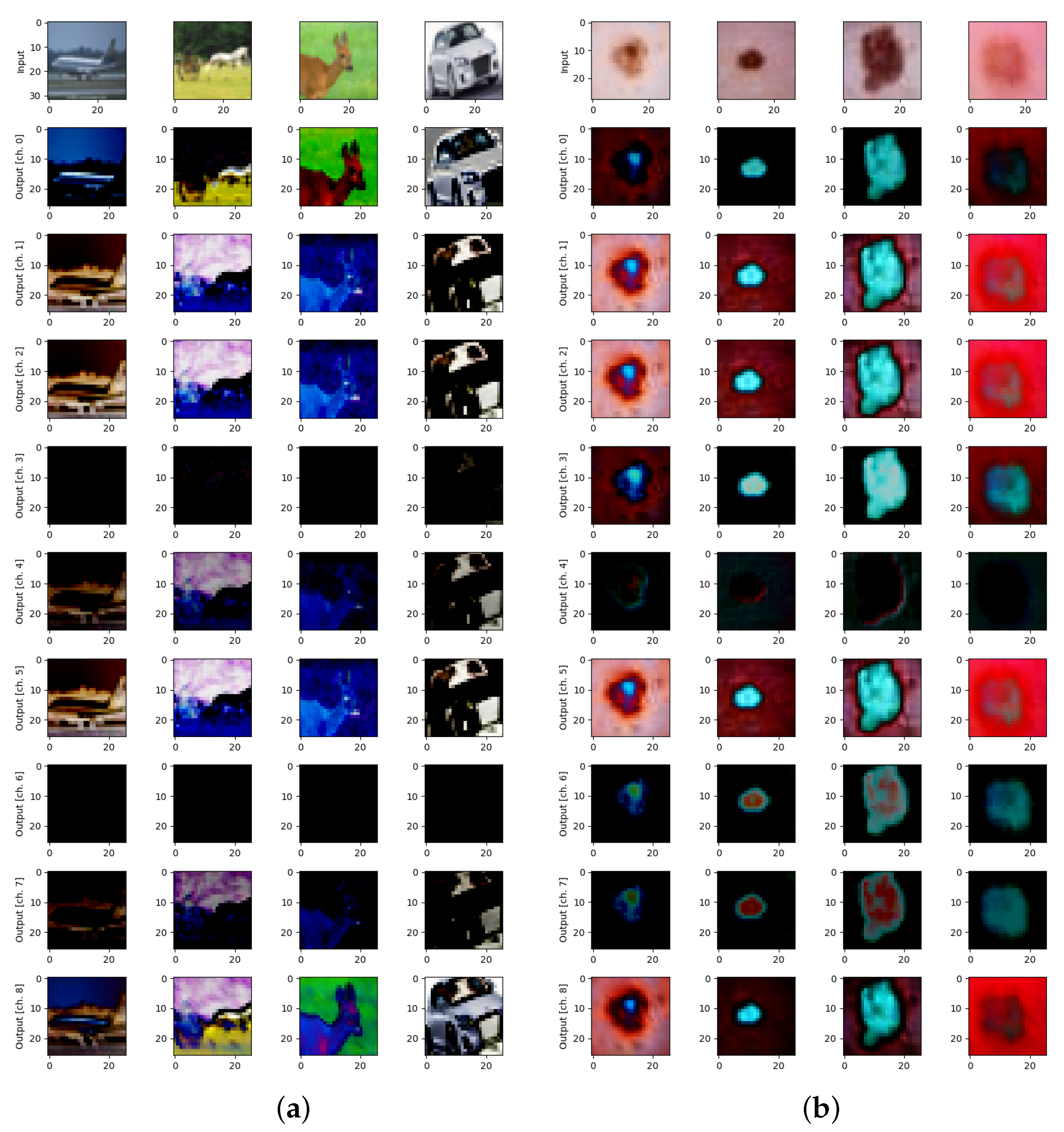
The CIFAR-10 dataset consists of 60,000 color images categorized into 10 classes, with each class containing 6000 images (Figure 1a, top row). The images in CIFAR-10 are of small size, specifically 32 × 32 pixels, and encompass a diverse range of objects commonly found in everyday life. The classes included in the dataset are as follows: airplane (various types of airplanes in different environments), automobile (cars, except for trucks), bird (various species of birds in diverse settings), cat (domestic cats in various poses and backgrounds), deer (in natural habitats), dog (various breeds and their environments), frog (often depicted in natural surroundings), horse (horses in different shapes), ship (different types of ships, including cargo and military vessels), truck (large trucks and their variants).
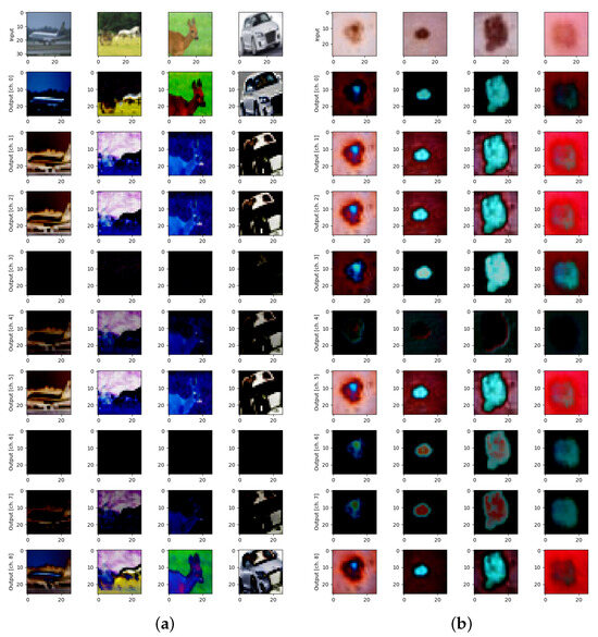
Figure 1.
Examples of datasets and quantum transformations for: (a) CIFAR-10 for Y and 9 qubits on 9 pixels, and (b) DermaMNIST for XY and 9 qubits on 9 pixels.
CIFAR-10 is typically divided into training and testing datasets to evaluate model performance effectively. The standard split is as follows: training set in 50,000 images and test set in 10,000 images. This division allows researchers to train their models on a substantial dataset while reserving a significant number of images for unbiased evaluation. All images are stored in RGB color format. Each image has a resolution of 32 × 32 pixels, making the dataset suitable for testing algorithms on smaller images, which is a common scenario in real-world applications.
CIFAR-10 is publicly available [33] and can be accessed through various platforms, including the official CIFAR website and machine learning libraries such as TensorFlow and PyTorch. This accessibility has made it a staple resource for researchers, educators, and practitioners in the field of computer vision.
3.1.2. DermaMNIST
The DermaMNIST dataset is part of the MedMNIST collection, specifically designed for medical image classification tasks [16,17]. DermaMNIST serves as a benchmark dataset for dermatological image classification, enabling the development and evaluation of machine learning models in the field of dermatology. With the increasing reliance on artificial intelligence for diagnostic purposes, this dataset facilitates research on skin disease recognition and contributes to the automation of dermatological assessments.
DermaMNIST contains a total of 10,000 images of skin lesions (Figure 1b, top row) representing a diverse range of dermatological conditions. Each image in the dataset is categorized into one of the following 7 classes:
- Melanoma: A type of skin cancer that develops from melanocytes, the cells responsible for skin pigmentation.
- Nevus: A benign pigmented lesion commonly known as a mole.
- Basal Cell Carcinoma (BCC): A common form of skin cancer that arises from basal cells in the skin.
- Actinic Keratosis: A precancerous condition characterized by rough, scaly patches on sun-exposed skin.
- Squamous Cell Carcinoma (SCC): A type of skin cancer originating from squamous cells, which make up the outer layer of skin.
- Dermatofibroma: A benign fibrous tumor of the skin.
- Vascular Lesion: Lesions associated with blood vessels, including conditions like hemangiomas.
Each image is uniformly sized at 28 × 28 pixels, providing a standardized input for machine learning models. The images are stored in standard RGB format. The DermaMNIST dataset is typically divided into training, validation, and test sets, allowing researchers to train models while evaluating their performance on unseen data. The standard split is as follows: training set: 8000 images, validation set: 1000 images, and test set: 1000 images. This division ensures that models can be effectively trained and fine-tuned while allowing for unbiased evaluation.
DermaMNIST can be utilized for various applications in medical image analysis, including but not limited to: developing CNNs for automatic classification of skin lesions; transfer learning by using pre-trained models on DermaMNIST to improve performance on other dermatological datasets; investigating the potential of machine learning in improving diagnostic accuracy and efficiency in dermatological practice.
The DermaMNIST dataset is publicly available and can be accessed through the MedMNIST repository. Researchers can utilize the dataset for algorithms, benchmarking against performance metrics of established state-of-the-art models.
3.2. Hardware
All experiments in this research were conducted on classical hardware due to a limited supply and high costs of physical quantum computers. The Pennylane framework [34] was used for assembling quantum circuits and running quantum simulations. We used the qml.devices.default_qubit simulation device from Pennylane, which represents an abstract standard qubit-based device. This research does not focus on any concrete type of actual quantum hardware and operates abstract qubit simulations. This enabled us to conduct a number of experiments that involve a significant number of quantum operations, which would be extremely costly if we used a physical quantum computer and would render this research borderline impossible for us.
Since a quantum simulator software was used for conducting experiments, it was impossible to assess the time metrics of quantum circuit executions. In this research, we operated under the assumption that the quantum part of the proposed HNN runs almost instantly compared to a classical part of the network.
Our experiments were run on a Kaggle platform using the TPU hardware accelerator “TPU VM v3-8” and are publicly available in the form of Jupyter Notebooks [35,36,37].
3.3. Data Preprocessing—Quantum Transformations
This research uses a variety of randomly assembled quantum circuits based on qubit rotation gates. The hypothesis behind the usage of random circuits is based on the assumption that randomness and noise introduced by a quantum transformation can be viewed as a non-classical data augmentation technique, which can be beneficial for model performance. This approach may be practical in the near future using NISQ quantum computers. In this research, combinations of two different types of quantum gates were used:
- Y-axis qubit rotation;
- X-axis qubit rotation.
In order to apply a quantum transformation over a single group of pixels, the value of each channel of each pixel is multiplied by and a quantum circuit is executed for every channel in order to produce resulting channels of transformed images. An in-depth description of the quanvolutional process can be found in its founding paper [7].
3.3.1. Y-Axis Quanvolutional Transformation
Y-axis quanvolutional transformation with stride 1 (Figure 1, in all rows except for the top one) was used among various possible quanvolutional operations that were described in details elsewhere [7,38] to create multi-channel quanvolutional input for image classification on CIFAR-10 (Figure 1a) and DermaMNIST (Figure 1b) datasets.
For this, the Pennylane framework [34] was used, where the qml.RY class represents a single-qubit rotation around the Y-axis (Figure 2a) (further details can be found elsewhere [22,38]). The matrix representation of a Y rotation by an angle is given by the following formula:

Figure 2.
Examples of quantum transformations implemented by Pennylane simulation software, Version: 0.36.0 [34] for: (a) Y with 4 qubits on 4 pixels, (b) XY with 4 qubits on 4 pixels, and (c) XY with 9 qubits on 9 pixels.
This matrix rotates a single qubit around the Y-axis of the Bloch sphere by an angle [34]. Here, the qml.RY quantum transformation of each pixel in the original image (Figure 1, top row) was used to create 9 (by the number of qubits) quantum-transformed images (Figure 1, all rows except for the top one).
3.3.2. X-Axis Quanvolutional Transformation
In the Pennylane framework, the qml.RX class represents a single-qubit rotation around the X-axis. The corresponding formula is given by the following formula:
3.3.3. XY-Axis Quanvolutional Transformation
The combined single-qubit rotation around the X-axis followed by a rotation around the Y-axis can be represented in the Pennylane framework by the combination of the qml.RX class and the qml.RY class (Figure 2b,c). These are sequential rotations, and the overall transformation is the product of these two matrices, :
The resulting matrix is given by the following formula:
This represents the combined rotation of a qubit around the X-axis followed by the Y-axis in a more compact and readable format.
3.4. Models
The following main aspects were taken into account for the formation of the models under investigation:
- Quantum transformations,
- Multibackbone ensembling.
Along with the classic baseline model, the following more complicated hybrid neural network (HNN) models with different numbers (n) of quantum channels (QCs) were used:
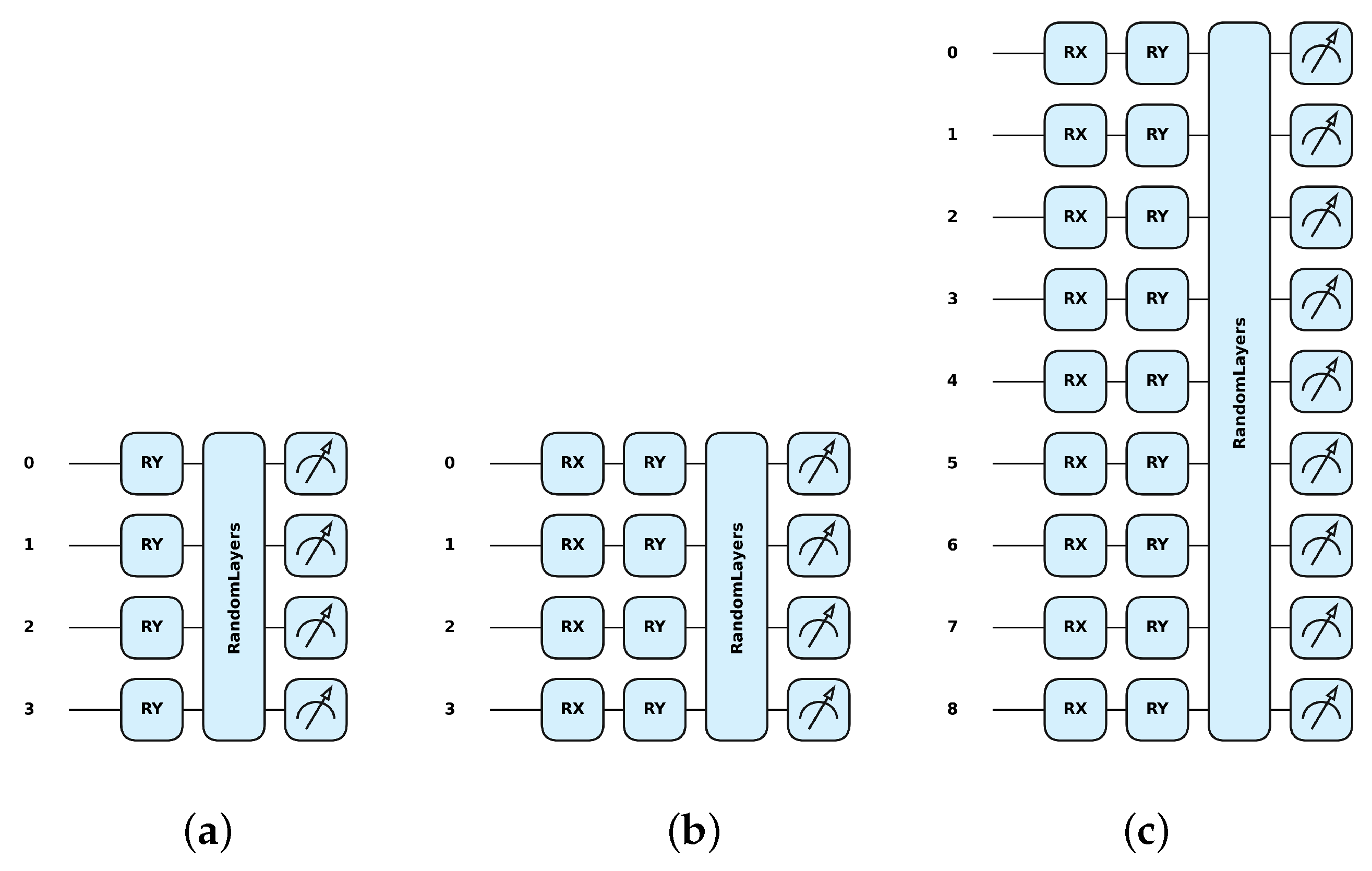
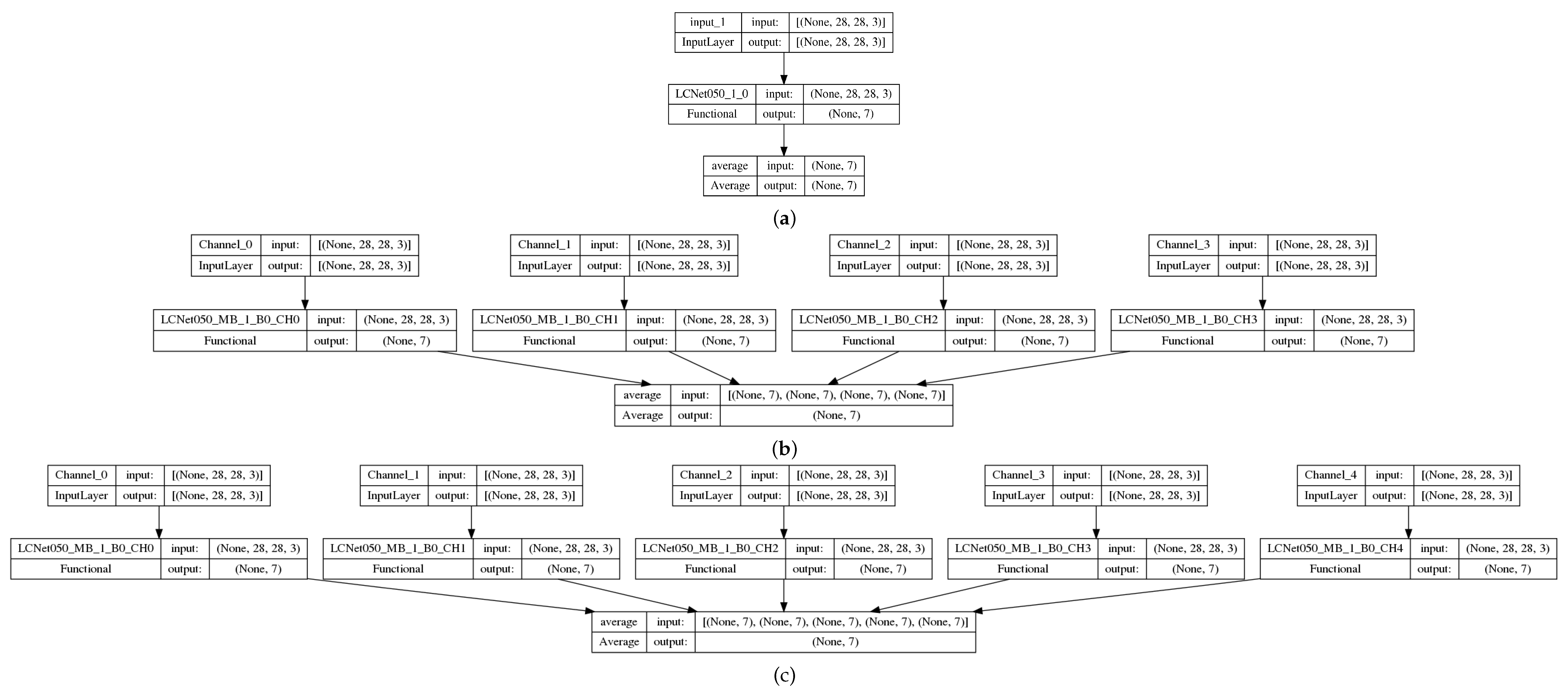
- Baseline: classic convolutional neural network (CNN), LCNet050 (Figure 3a) with the single input channel of the original images;
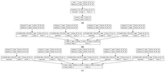 Figure 3. Examples of neural networks: (a) baseline with a single input channel (original image) and LCNet050 backbone, and (b) QC4 with 4 input channels (4 quantum preprocessed data) and 4 LCNet050 backbones, and (c) QC5 with 5 input channels (4 quantum preprocessed data + original image) and 5 LCNet050 backbones.
 - HNN-QC4: hybrid (quantum-classic) neural network (HNN)(Figure 3b) with multiple (actually 4) backbones of LCNet050 CNN with the 4 quanvolutional input channels (QC4);
- HNN-QC5: HNN with multiple (5) backbones of LCNet050 CNN with 5 input channels: QC4 and 5-th input channel of the original images (Figure 3c);
- HNN-QCn: HNN with multiple (n) backbones of LCNet050 CNN with n input channels in various combinations of QC with/without the original images (Table 1).
 Table 1. HNN-QCn: multiple backbones of LCNet050 CNN with n input channels in various combinations of the QC and the original (O1) input images.
LCNet050 is used here as an example of a small and quite efficient family of CNN models that demonstrates excellent performance despite the small size [39]. It was used due to their open-source availability and detailed descriptions elsewhere [40]. Further research will be dedicated to the investigation of other CNNs that can be used to understand their influence on general performance.
3.5. Workflow
During the training and validation phases of the workflow, several standard performance metrics were employed to evaluate the models. These metrics included training and validation loss, which measure how well the model fits the training data and performs on unseen validation data. Loss is a quantitative indicator calculated using a Categorical Cross-Entropy loss function that reflects the error between the model’s predictions and the actual labels. Training and validation accuracy were also tracked to quantify the proportion of correctly classified samples during the training and validation stages, providing an intuitive measure of the model’s predictive success. Additionally, the area under the curve (AUC) for the receiver operating characteristic (ROC) curve was used [41]. The ROC-AUC metric evaluates the model’s ability to distinguish between classes by plotting the true positive rate (sensitivity) against the false positive rate (1-specificity) across different classification thresholds. The micro-average AUC aggregates metrics globally by considering all instances, while the macro-average AUC computes metrics for each class individually and then averages them, treating all classes equally regardless of sample size.
The Adam optimizer was utilized for training a gradient-based optimization algorithm designed for deep learning with the following parameters [42]:
- = 0.9: controls the exponential decay rate for the first moment estimate (similar to momentum),
- = 0.999: controls the exponential decay rate for the second moment estimate (related to variance),
- learning rate = : determines the step size during weight updates,
- batch size = various (see below): the number of training samples processed before the model updates its weights.
The training spanned 200 epochs, where one epoch corresponds to one complete pass through the training dataset.
The quantum transformations applied in the HNN-QCn architecture involved 4 (W4) and 9 (W9) qubits, representing the quantum processing units used for feature extraction. The receptive field was set to 2 × 2 pixels for W4 and 3 × 3 pixels for W9, defining the size of the input area processed by each quantum transformation, with a stride of 1, indicating the step size for the transformation across the input data.
A cross-validation (CV) setup [43] was adopted for training, which ensures robust model evaluation by reducing overfitting and providing reliable performance estimates. The training subset of each dataset was divided six-fold, creating six subsets where the model was trained on five folds and validated on the remaining one. Validation metrics were computed for each fold, and the mean and standard deviations were calculated. This process identified the best-performing model by selecting the one with the highest AUC score. Statistical reliability was assessed by analyzing the variability of the metrics across folds, ensuring that the results were consistent and generalizable.
4. Results
This section provides the description of the experimental results obtained for different models (baseline, HNN-QC4, HNN-QC5, and other HNN-QCn models) trained on the CIFAR-10 and DermaMNIST datasets with their interpretation and the experimental conclusions that can be drawn.
Here, we analyze the results presented in the tables and visualized by figures (for better comprehension) below for different models trained on the CIFAR-10 and DermaMNIST datasets. The analysis focuses on trends observed across batch sizes, models, and their impact on performance metrics like AUC and accuracy.
4.1. CIFAR-10
4.1.1. Baseline Model
AUC and accuracy values (mean ± std) for the baseline model on the CIFAR-10 dataset are shown in Table 2 (here and below the highest value of each metric is emphasized by the bold font) and Figure 4 for AUC and Figure 5 for accuracy.
Table 2.
AUC and accuracy values (mean ± std) for the baseline model on the CIFAR-10 dataset.
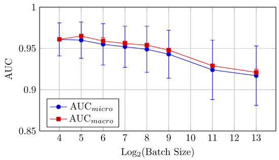
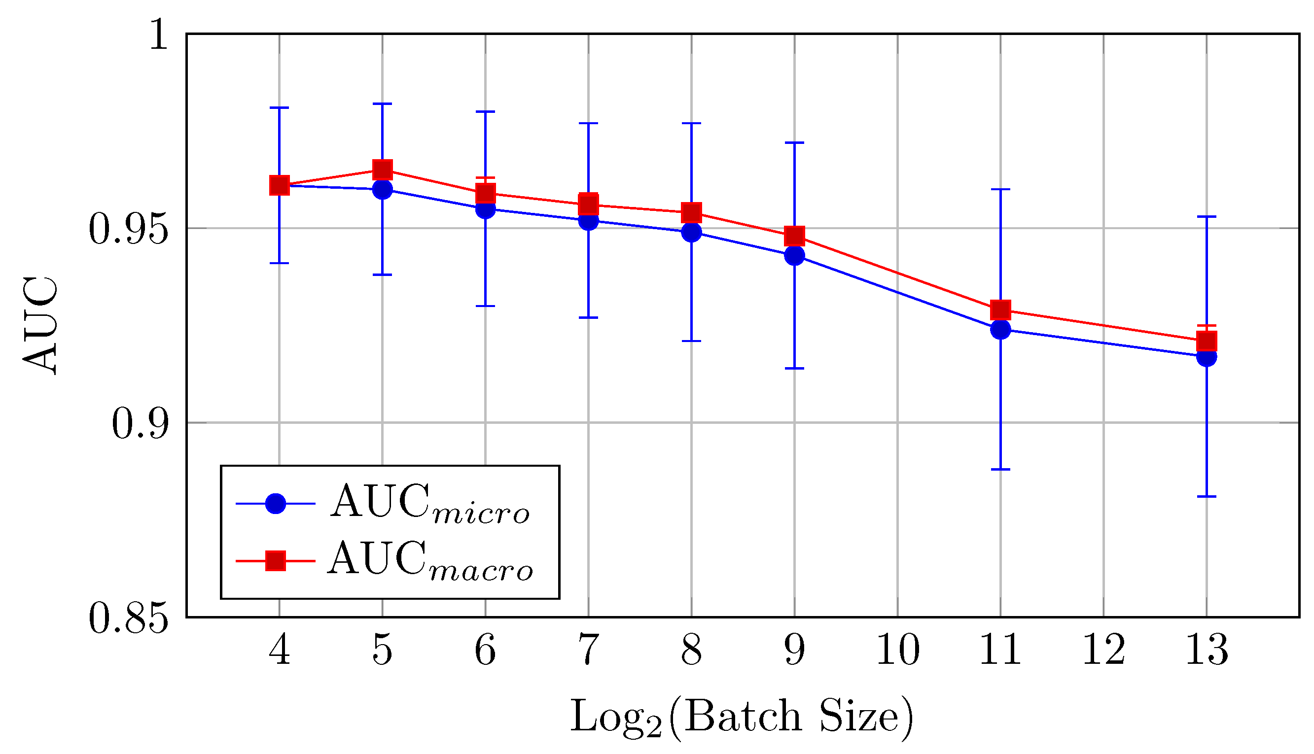
Figure 4.
AUCmicro and AUCmacro vs. Log2(Batch Size) for the baseline model on CIFAR-10 dataset (Table 2).
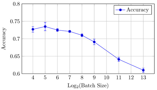
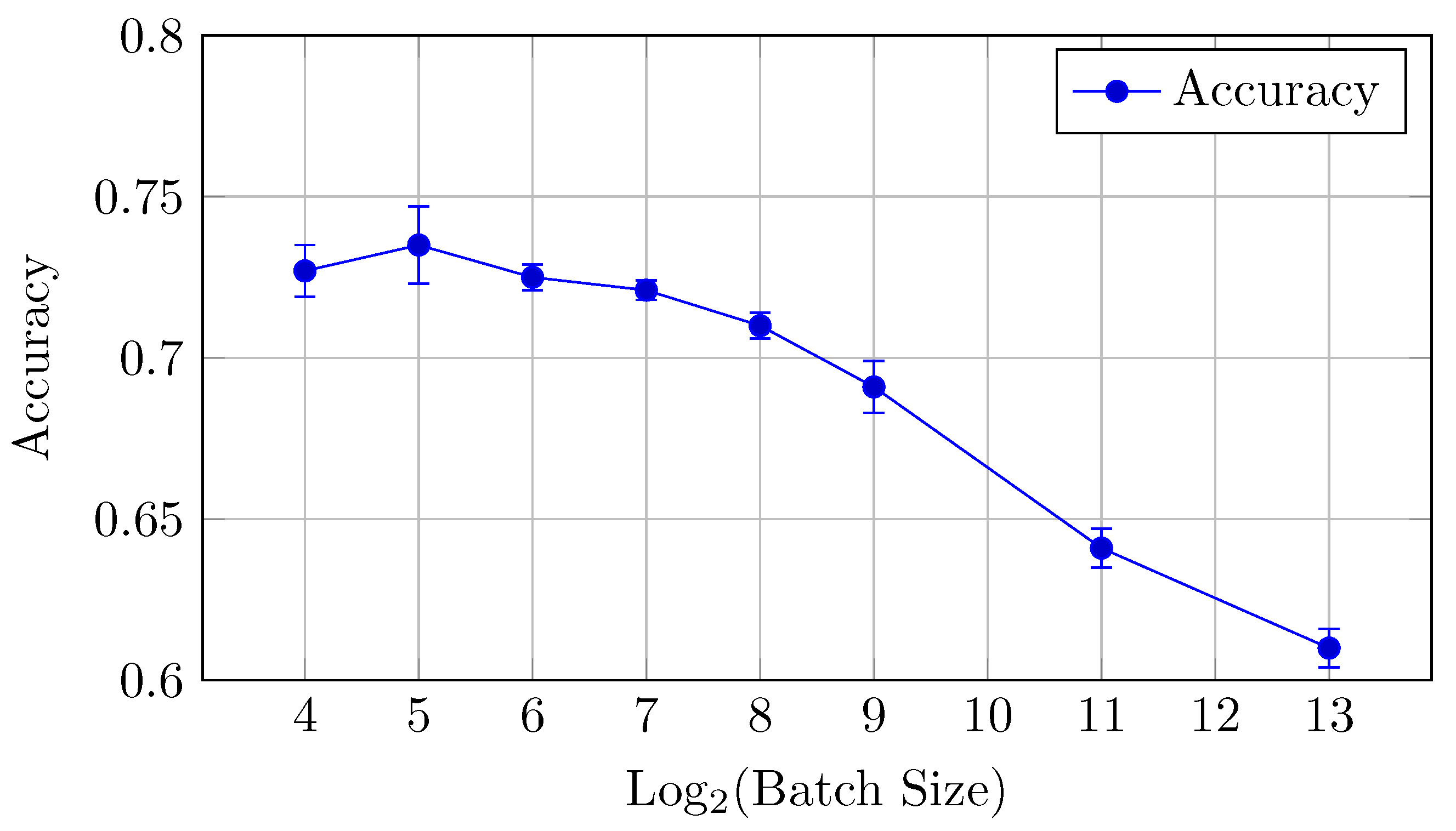
Figure 5.
Accuracy vs. Log2(Batch Size) for the baseline model on CIFAR-10 dataset (Table 2).
The baseline model for CIFAR-10 exhibits a decreasing trend in both AUC (micro and macro) and accuracy as the batch size increases from 16 to 8192. Notably, the AUCmicro drops from 0.961 for a batch size of 16 to 0.917 for a batch size of 8192, while the accuracy similarly decreases from 0.727 to 0.610.
AUC: There is a clear downward trend, with the highest AUCmicro and AUCmacro values observed for smaller batch sizes (16 and 32). Both metrics drop as the batch size increases beyond 64 (but the difference between the mean values is in the limits of standard deviation up to batch size 512), indicating that smaller batch sizes might be more effective for optimizing AUC in the baseline model. AUCmicro and AUCmacro values proved to be very close for all batch sizes in terms of our experiments, especially for a batch size of 16 elements, which indicates that the model performance on all classes of the dataset is very consistent and there is a small difference in classification accuracy between all specific classes.
Accuracy: Similarly, accuracy starts at 0.727 for a batch size of 16 and steadily decreases as the batch size increases (but the difference between the mean values is in the limits of standard deviation up to batch size 128). The best performance is achieved at a batch size of 32, with an accuracy of 0.735.
Overall, small batch sizes (16 or 32) seem to yield better performance in both AUC and accuracy for the baseline model.
Code samples of the experiment setup and results are available on the Kaggle platform [35].
4.1.2. HNN-QC4 Model
AUC and accuracy values (mean ± std) for the HNN-QC4 model on the CIFAR-10 dataset are shown in Table 3 and Figure 6 for AUC and Figure 7 for accuracy.
Table 3.
AUC and accuracy values (mean ± std) for the HNN-QC4 model on the CIFAR-10 dataset.

Figure 6.
AUCmicro and AUCmacro vs. Log2(Batch Size) for the HNN-QC4 model on the CIFAR-10 dataset (Table 3).
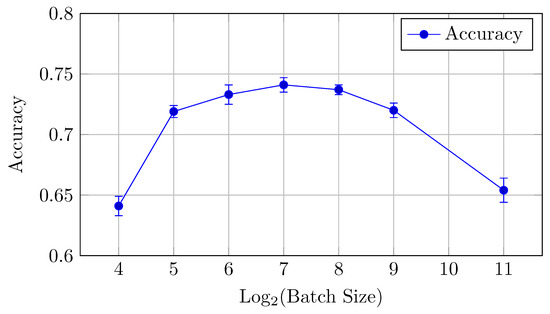
Figure 7.
Accuracy vs. Log2(Batch Size) for the HNN-QC4 model on CIFAR-10 dataset (Table 3).
For the HNN-QC4 model, the AUC and accuracy values show an improvement compared to the baseline model, especially in the mid-range batch sizes (32 to 256). The performance is relatively stable for batch sizes between 64 and 256, with minor variations.
AUC: The AUC values are quite stable for batch sizes between 64 and 256, with AUCmicro hovering around 0.955. This consistency of AUC suggests that the HNN-QC4 model is less sensitive to batch size changes within this range. Also, a very small difference between AUCmicro and AUCmacro values across all investigated batch sizes indicates stable consistency of the model performance across all classes of the dataset.
Accuracy: The highest accuracy is achieved with a batch size of 128 (0.741), showing that mid-sized batch sizes perform best for this model. However, accuracy begins to drop at batch sizes lower than 64 and higher than 256.
Code samples of the HNN-QC4 architecture setup and full experiment results are available on the Kaggle platform [36].
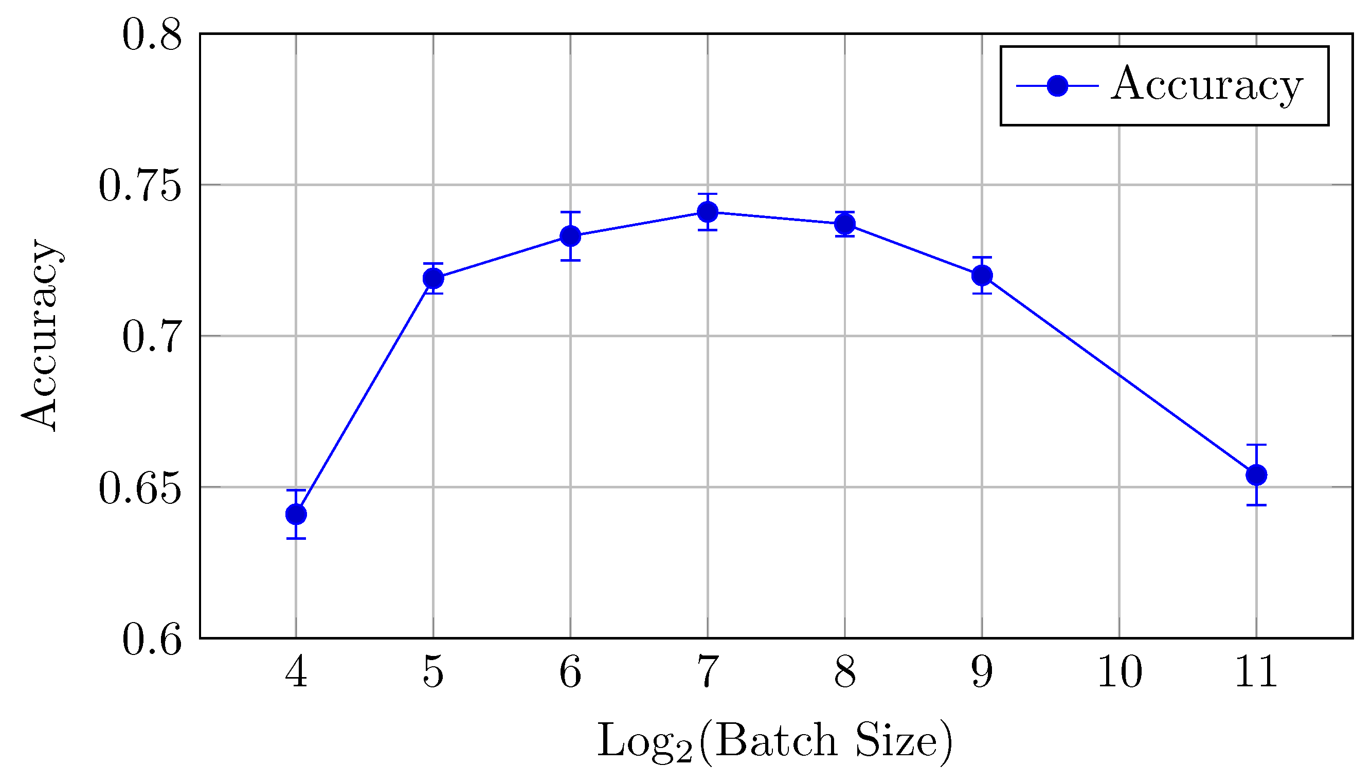
4.1.3. HNN-QC5 Model
AUC and accuracy values (mean ± std) for the HNN-QC5 model on the CIFAR-10 dataset are shown in Table 4 and Figure 8 for AUC and Figure 9 for accuracy.
Table 4.
AUC and accuracy values (mean ± std) for the HNN-QC5 model on CIFAR-10 dataset.
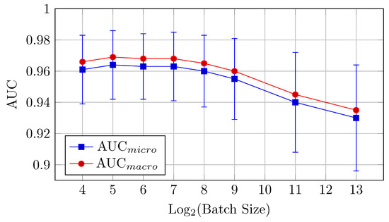
Figure 8.
AUCmicro and AUCmacro vs. Log2(Batch Size) for the HNN-QC5 model on CIFAR-10 dataset (Table 4).

Figure 9.
Accuracy vs. Log2(Batch Size) for the HNN-QC5 model on CIFAR-10 dataset (Table 4).
AUC: The highest AUC values are observed with batch sizes of 16 and 32, where AUCmicro reaches 0.964 and AUCmacro hits 0.969. This model performs better at small batch sizes but the difference between the mean values is in the limits of standard deviation up to batch size 512. The relative proximity of AUCmicro and AUCmacro values across all samples also indicates the stability of the model performance across all classes in the dataset.
Accuracy: The HNN-QC5 model also outperforms the others in terms of accuracy, with the highest value of 0.769 observed at a batch size of 128. However, the model maintains strong performance across batch sizes between 32 and 256.
This model demonstrates that small to medium batch sizes (16 to 128) yield the best results for AUC and accuracy. Performance declines at larger batch sizes (512, 2048), following a similar trend to the other models.
Code samples of HNN-QC5 architecture setup and full experiment results are available on the Kaggle platform [37].
4.1.4. Comparison of Models on CIFAR-10 Dataset
Overall, comparing all models on the CIFAR-10 dataset, one can observe that the HNN-QC5 model exhibits the best overall performance among the models tested on CIFAR-10. Both AUC and accuracy are consistently higher than those observed for the baseline and HNN-QC4 models. For example, comparing the best AUC and accuracy values (mean ± std) for various batch sizes for the different HNN-QCn models on the CIFAR-10 dataset (Table 5), one can note the tendency of the higher AUC and accuracy mean values and the lower values of standard deviation for accuracy with an increase in the backbones and QC inputs.
Table 5.
The best AUC and accuracy values (mean ± std) for the different HNN-QCn models on CIFAR-10 dataset for various batch sizes.
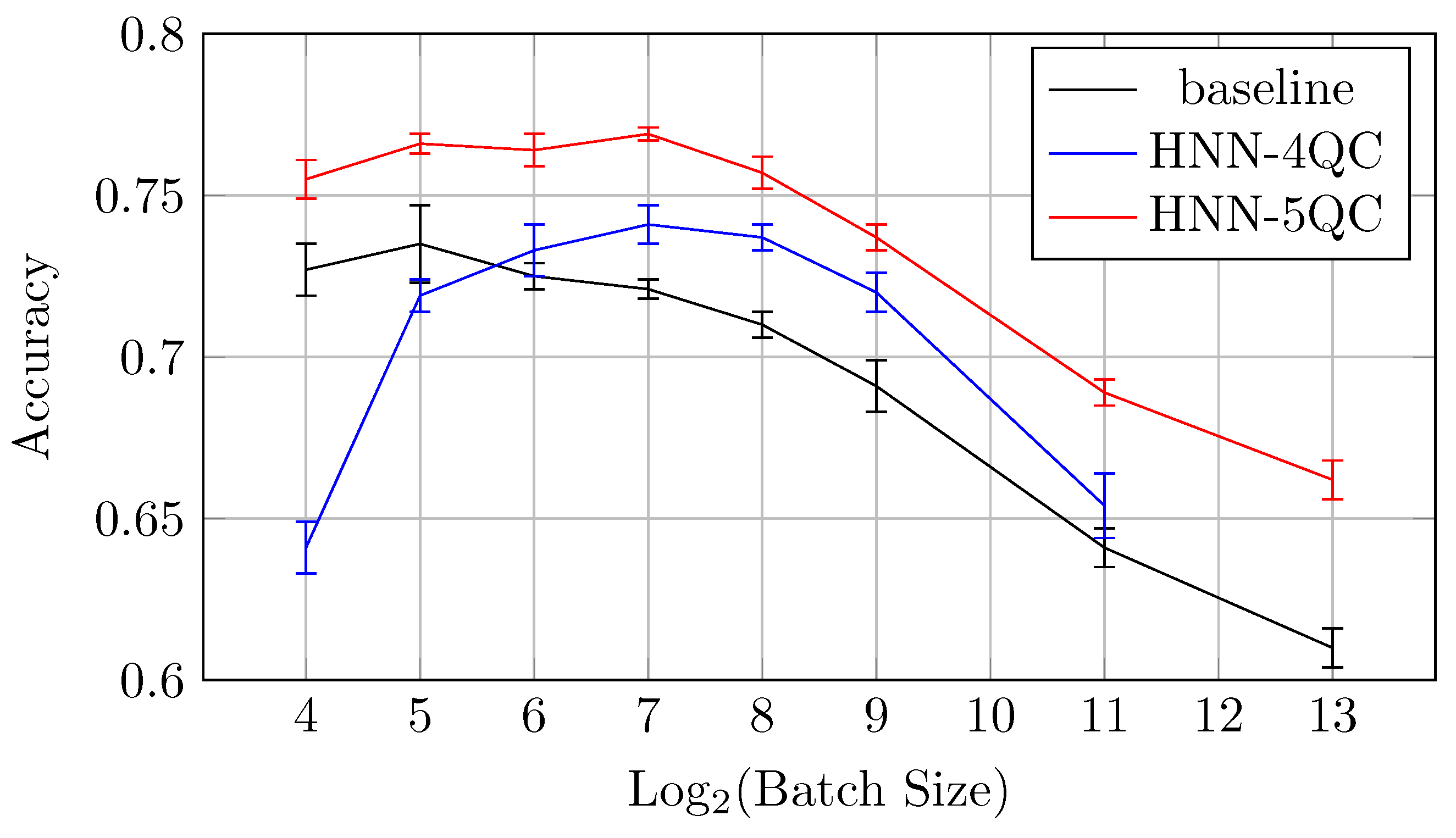
Also, the mean accuracy values become higher with an increase in the backbones and QC inputs for batch sizes of 64 and higher. This is demonstrated by Figure 10, which shows accuracy vs. batch size charts for NHH-QC4, HNN-QC5 and baseline models on the CIFAR10 dataset. This chart was built based on the accuracy values of inspected models on various batch sizes on the CIFAR10 dataset; these data are shown in Table 2, Table 3 and Table 4. It can be seen that the accuracy demonstrated by HNN-QC5 is consistently higher compared to the accuracy demonstrated by HNN-QC4, and the accuracy of HNN-QC4 is consistently higher compared to the accuracy of the baseline model for batch sizes of 64 and higher.

These results motivated further similar investigations on specific datasets that are of great importance for practice, for example, one of the MedMNIST datasets, specifically DermaMNIST.
4.2. DermaMNIST
4.2.1. Baseline Model
AUC and accuracy values (mean ± std) for the baseline model on the DermaMNIST dataset are shown in Table 6 and Figure 11 for AUC and Figure 12 for accuracy.
Table 6.
AUC and accuracy values (mean ± std) for the baseline model on the DermaMNIST dataset.
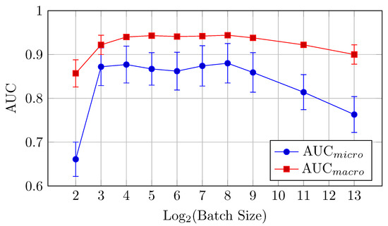
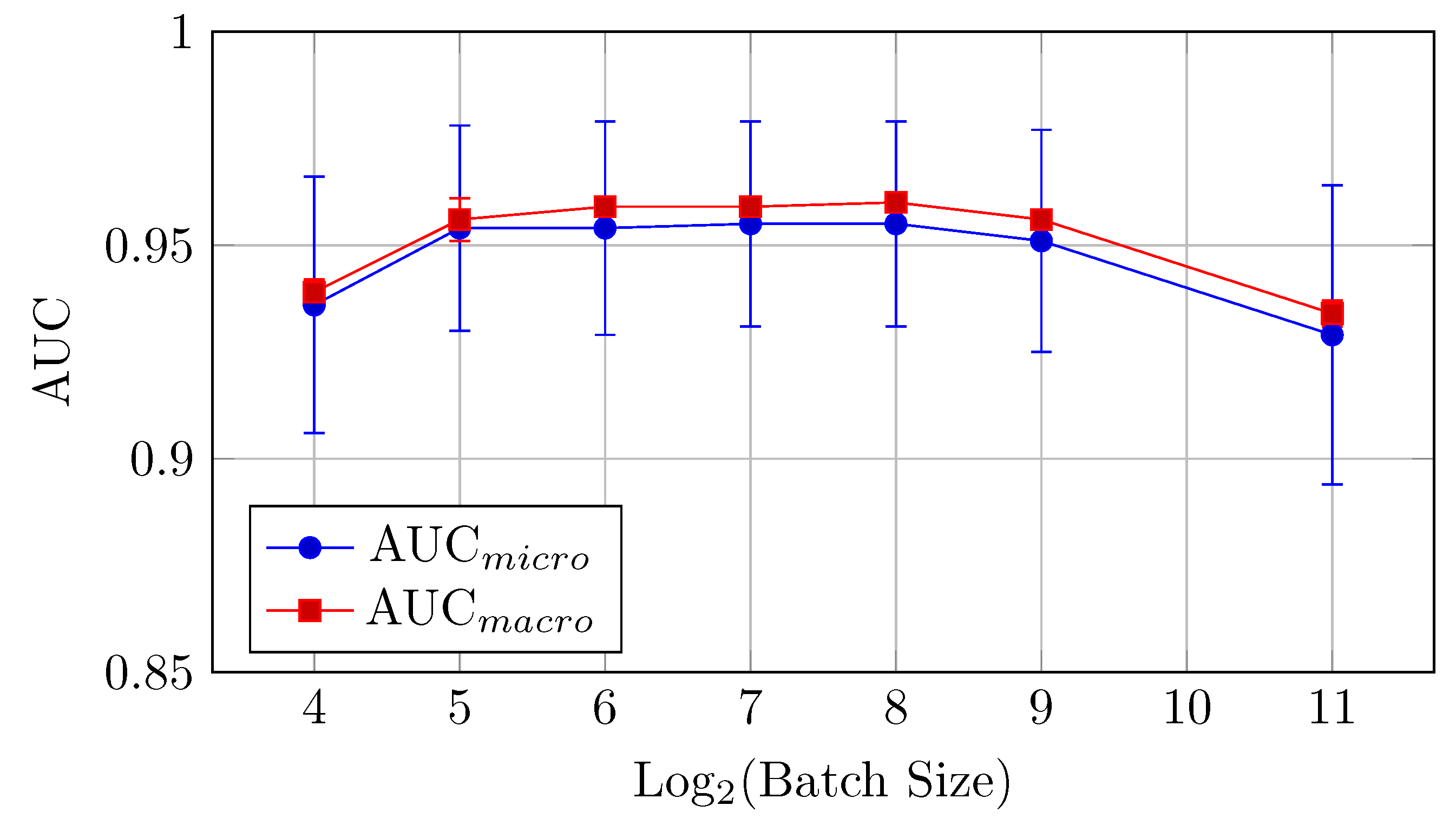
Figure 11.
AUCmicro and AUCmacro vs. Log2(Batch Size) for the baseline model on the DermaMNIST dataset (Table 6).

Figure 12.
Accuracy vs. Log2(Batch Size) for the baseline model on DermaMNIST dataset (Table 6).
For the DermaMNIST dataset, the baseline model shows a gradual improvement in performance as the batch size increases from 4 to 256, after which performance declines.
AUC: The highest AUC values are observed at a batch size of 256, with AUCmicro reaching 0.880 and AUCmacro at 0.944. This suggests that a larger batch size is beneficial for AUC for the baseline model.
Accuracy: The highest accuracy value of 0.701 is obtained with a batch size of 128. Although batch sizes of 256 and 128 perform similarly, 128 offers a marginally better trade-off between AUC and accuracy.
This suggests that a batch size of 128 provides the best balance between AUC and accuracy for the baseline model.
4.2.2. HNN-QC4 Model
AUC and accuracy values (mean ± std) for the HNN-QC4 model on the DermaMNIST dataset are shown in Table 7 and Figure 13 for AUC and Figure 14 for accuracy.
Table 7.
AUC and accuracy values (mean ± std) for the HNN-QC4 model on DermaMNIST dataset.
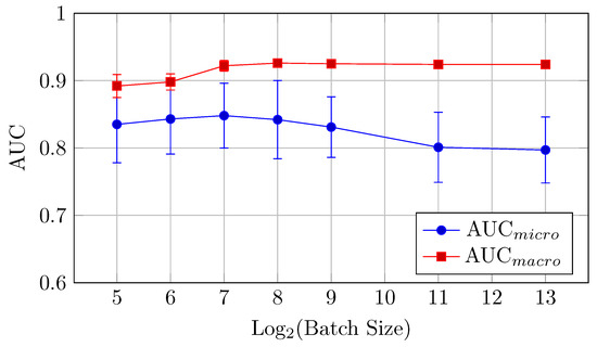
Figure 13.
AUCmicro and AUCmacro vs. Log2(Batch Size) for the HNN-QC4 model on DermaMNIST dataset (Table 7).
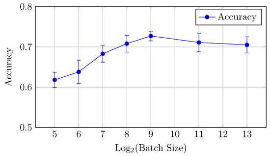
Figure 14.
Accuracy vs. Log2(Batch Size) for the HNN-QC4 model on DermaMNIST dataset (Table 7).
AUC (micro and macro): The highest AUC values are achieved with batch sizes of 128 and 256, with AUCmicro at 0.848 with a batch size of 128 and AUCmacro at 0.926 with a batch size of 256.
Accuracy: The best accuracy (0.727) is observed at a batch size of 512. In contrast to the baseline model, performance reaches its peak at mid-to-high sized batches (512–2048) and declines on larger batch sizes. This is slightly better than the baseline model, confirming the strength of the HNN-QC4 architecture for this dataset.
Thus, a batch size of 512 offers the best performance in terms of accuracy, while 256 is preferable for AUC.
The HNN-QC4 model generally outperforms the baseline model on DermaMNIST in classification accuracy, especially for larger batch sizes.
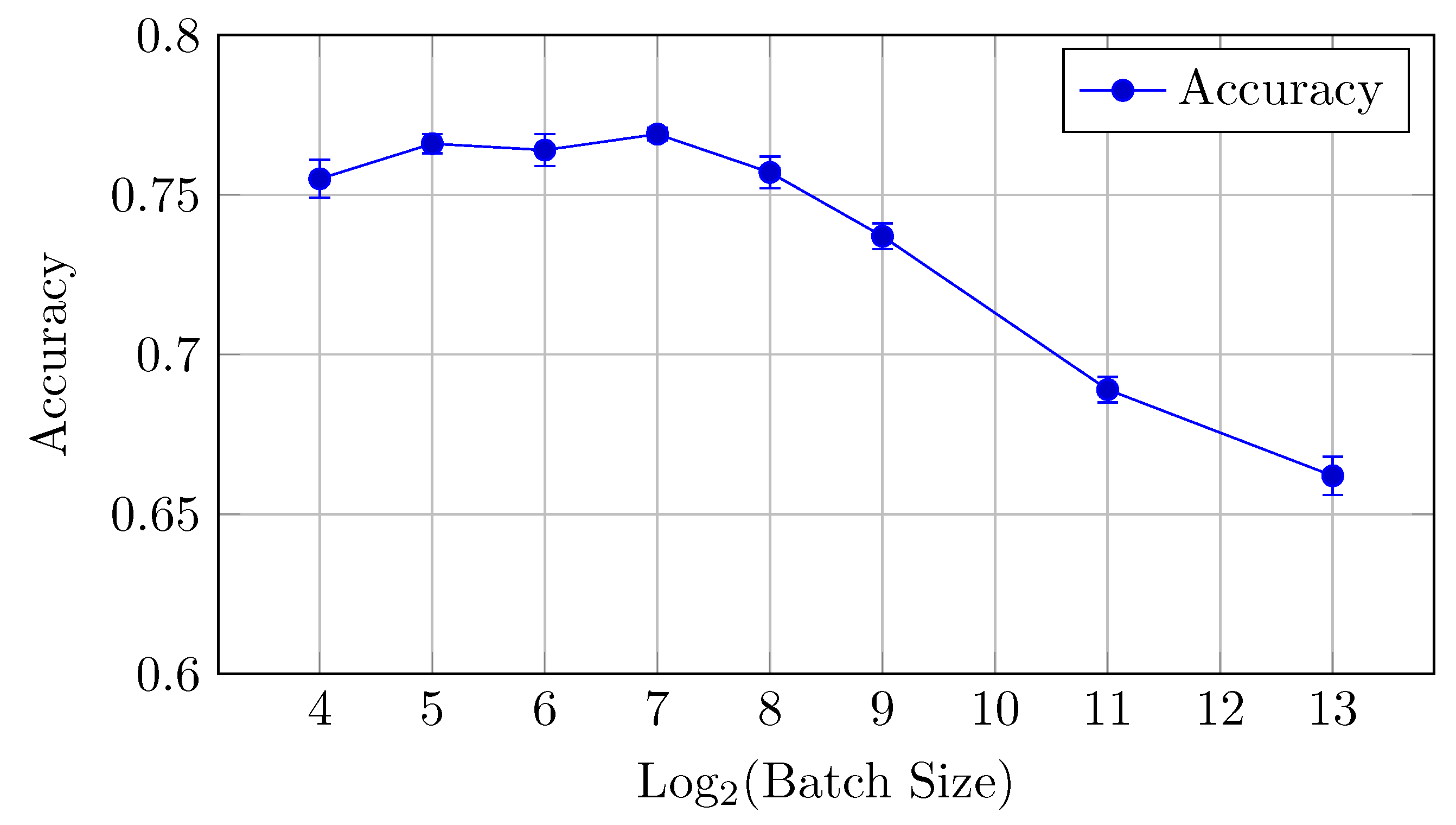
4.2.3. HNN-QC5 Model
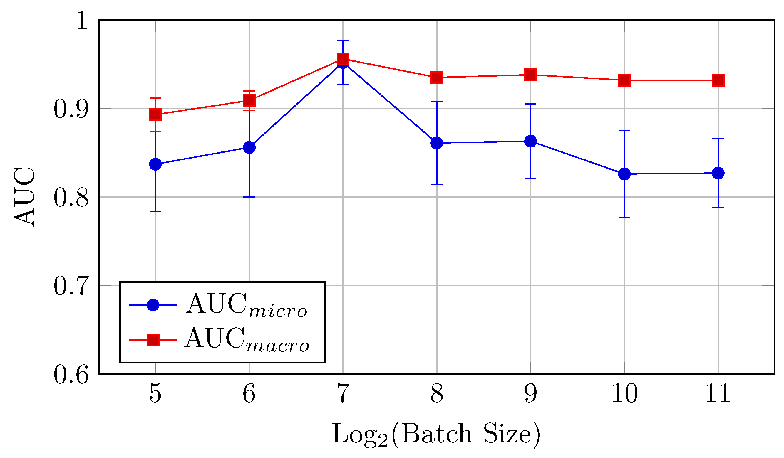
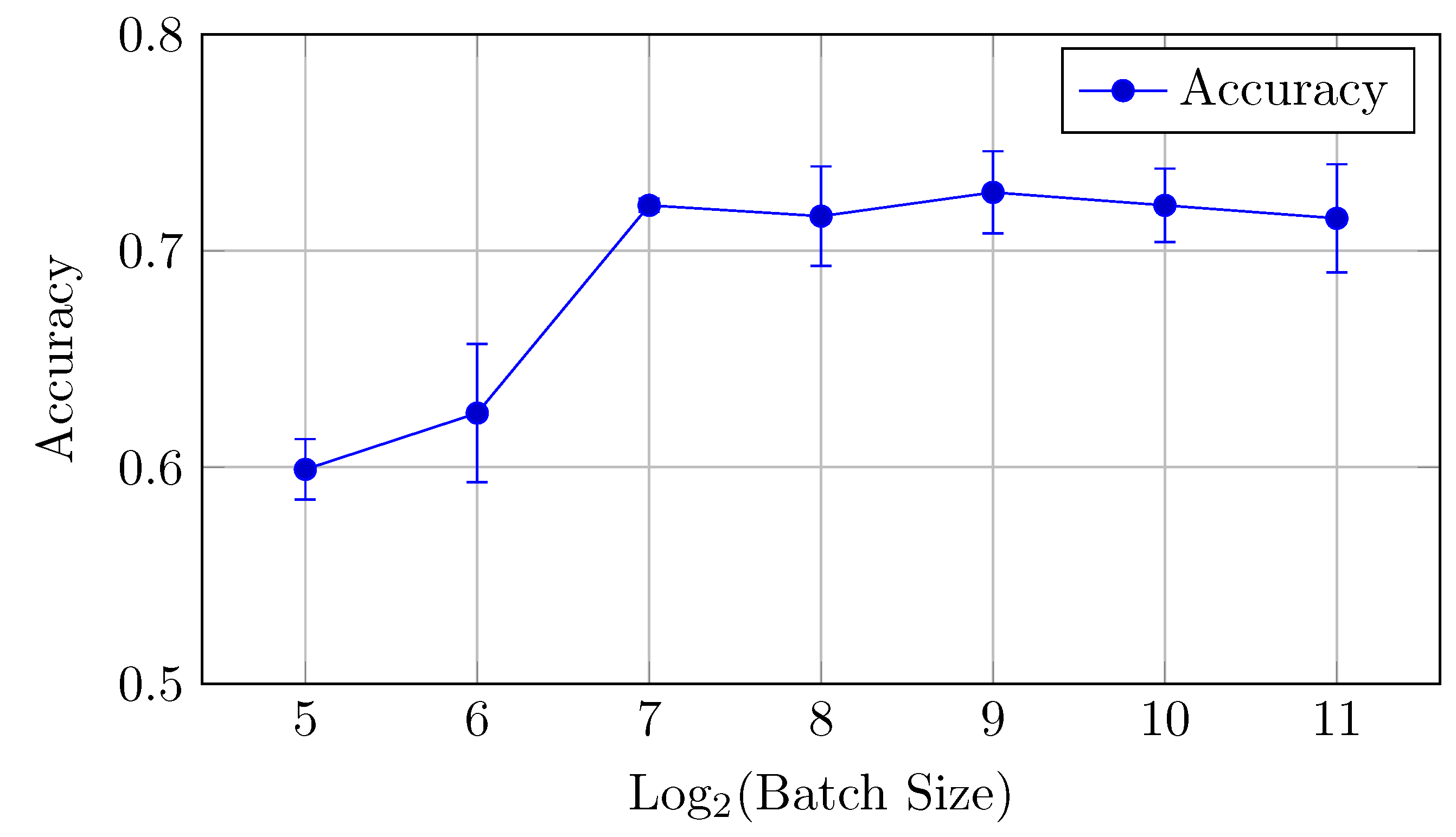
AUC and accuracy values (mean ± std) for the HNN-QC5 model on the DermaMNIST dataset are shown in Table 8 and Figure 15 for AUC and Figure 16 for accuracy.
Table 8.
AUC and accuracy values (mean ± std) for the HNN-QC5 model on the DermaMNIST dataset.
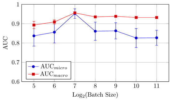
Figure 15.
AUCmicro and AUCmacro vs. Log2(Batch Size) for the HNN-QC5 model on the DermaMNIST dataset (Table 8).
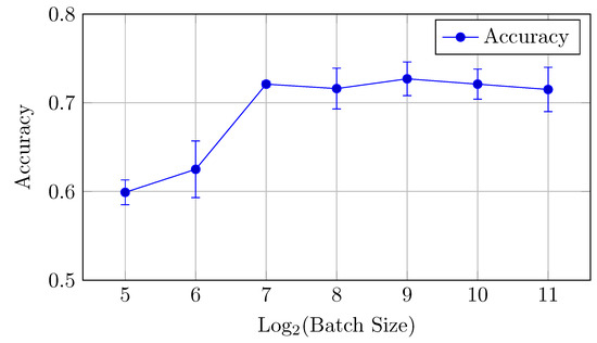
Figure 16.
Accuracy vs. Log2(Batch Size) for the HNN-QC5 model on the DermaMNIST dataset (Table 8).
The HNN-QC5 model, in terms of both AUC (micro and macro) and classification accuracy, follows trends of the HNN-QC4 model with peak AUC (both micro and macro) at a batch size of 128 elements (0.952 and 0.956, respectively), and the highest level of accuracy is reached at higher batch sizes (512–2048) with a peak of 0.727 at a batch size of 512. In addition, a maximum stability of the model performance was reached at a batch size of 128, which is indicated by extremely close values of AUCmicro and AUCmacro.
In general, the HNN-QC5 model outperforms the baseline model in AUCmacro and classification accuracy. Also, the more complex NHH-QC5 model outperforms the more simple HNN-QC4 architecture in AUC and reaches the same level of accuracy thus rendering its results superior to both of the previously inspected architectures.
4.2.4. Comparison of Models on DermaMNIST Dataset
Overall, by comparing all models on the DermaMNIST dataset, one can observe that the HNN-QC5 model demonstrates the best overall performance among the models tested on DermaMNIST. Both AUC and accuracy are consistently higher (or equal for accuracy for HNN-QC4) than those observed for the baseline and HNN-QC4 models. For example, again, comparing the best AUC and accuracy values (mean ± std) for various batch sizes for the different HNN-QCn models on the CIFAR-10 dataset (Table 9), one can note the tendency of the higher AUC and accuracy mean values to result in an increase in the backbones and QC inputs.
Table 9.
The best AUC and accuracy values (mean ± std) for the different HNN-QCn models on the DermaMNIST dataset for various batch sizes.
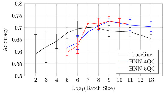
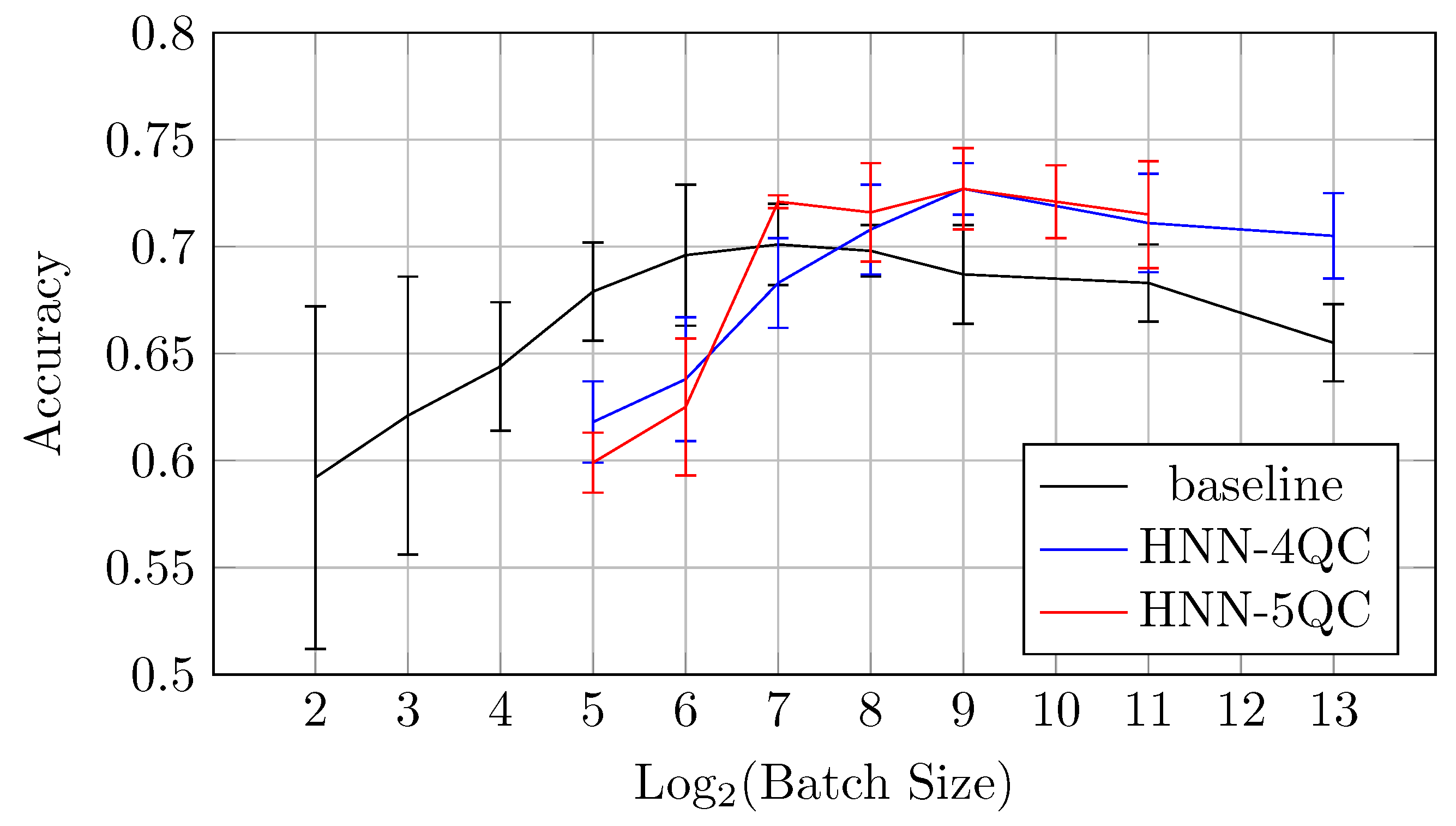
Also, the mean accuracy values become higher with an increase in the backbones and QC inputs for all batch sizes higher than 128. This is demonstrated by Figure 17, which shows accuracy vs. batch size charts for NHH-QC4, HNN-QC5 and baseline models on the DermaMNSIT dataset. This chart was built based on the accuracy values of inspected models with various batch sizes on the DermaMNIST dataset; these data are shown in Table 6, Table 7 and Table 8. It can be seen that the accuracy demonstrated by HNN-QC5 and HNN-QC4 is consistently higher compared to the accuracy of the baseline model for batch sizes higher than 128. It is also worth noting that the difference in the accuracy between HNN-QC4 and HNN-QC5 is insignificant and lies within the limits of standard deviations on all batch sizes higher than 128.
4.2.5. Other HNN-QCn Models
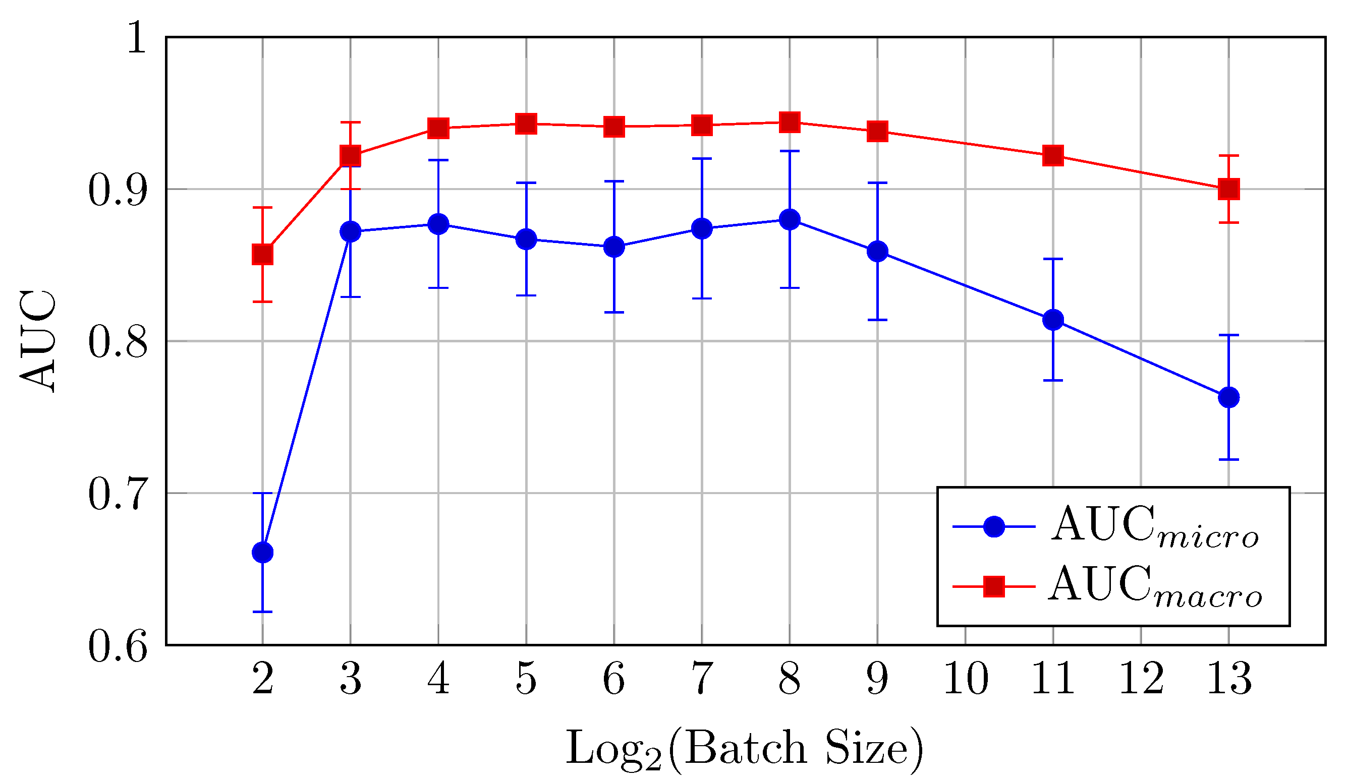
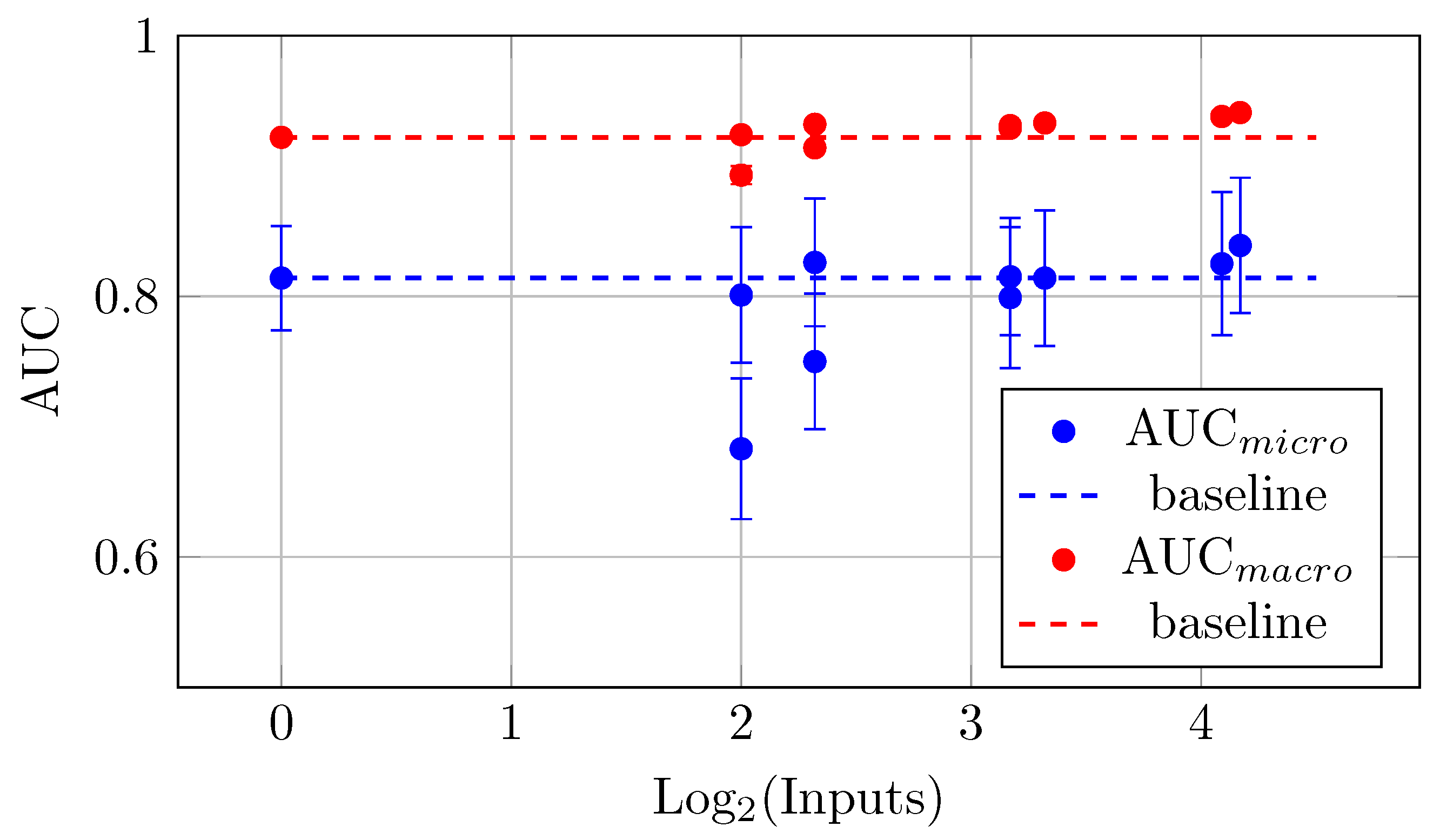
These results motivated further investigations of the influence of an additional increase in the backbones and QC inputs, for example, on the practically important DermaMNIST dataset. As far as AUC and accuracy values are within the limits of standard deviations for batch sizes higher than 512 and training time is significantly smaller for the larger batch sizes, further experiments were performed for the batch size 2048. The higher batch size was impossible for some of the bigger models due to the limits of the available memory.
The AUC and accuracy value (mean ± std) metrics presented in Table 10 indicate the performance of various models with different backbone and QC input values on the DermaMNIST dataset.
Table 10.
AUC and accuracy values (mean ± std) for the different HNN-QCn models on DermaMNIST dataset for the batch size 2048.
The models with more backbones and QC inputs show a more significant increase in the mean AUC values. This trend indicates that as the number of inputs increases (up to 18 in this case), the AUC values tend to improve. This indicates a positive correlation between the number of backbones and QC inputs and the measured mean AUC values. For instance, the maximal mean AUC values (Table 10 and Figure 18) were observed for the biggest model YW4 + XYW4 + XYW9 + O1 with 0.839 ± 0.052 (for AUCmicro) and 0.941 ± 0.001 (for AUCmacro).
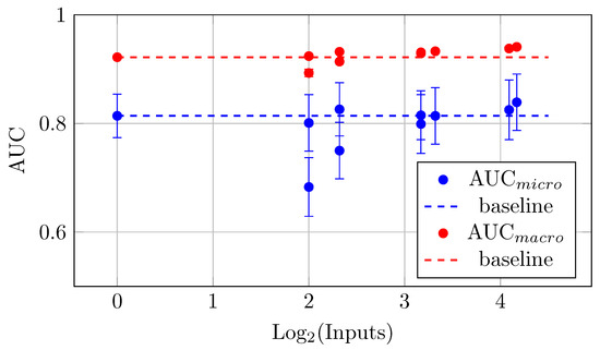
Figure 18.
AUCmicro and AUCmacro vs. Log2(Batch Size) for the different HNN-QCn models on DermaMNIST dataset for the batch size 2048 (Table 10).
As for the impact of multiple backbones and QC inputs on accuracy, the same and a more pronounced trend can be observed. The largest model YW4 + XYW4 + XYW9 + O1 also achieved the highest accuracy of 0.734 ± 0.020, which reflects a trend where increased input leads to better accuracy (Table 10 and Figure 19). Notably, while accuracy generally improves with more inputs, the rate of improvement may vary across different models.
Figure 19.
Accuracy vs. Log2(Batch Size) for the different HNN-QCn models on DermaMNIST dataset for the batch size 2048 (Table 10).
In general, models with additional backbones and QC inputs tend to show improved AUC and accuracy values, suggesting that increasing model complexity may lead to better performance.
5. Discussion
The more detailed analysis of the data on CIFAR-10 (Table 2, Table 3 and Table 4) and DermaMNIST (Table 6, Table 7, Table 8, Table 9 and Table 10) reveals several insights into the performance of different hybrid neural networks (HNNs) and the impact of various configurations such as quantum channels, backbone networks, and batch sizes.
The addition of quantum channels with multiple backbones consistently improves the models’ AUC and accuracy, showing higher performance across both datasets.
For both datasets, mid-range batch sizes (e.g., 128–256) tend to yield better AUC values, while slightly bigger batch sizes (e.g., 512–2048) tend to perform better in terms of accuracy. Larger batch sizes (>2048) generally lead to performance saturation (sometimes small degradation in the limits of the standard deviation). These findings suggest that increasing model complexity (through quantum transformations and multiple backbones) generally improves performance, but the optimal batch size is crucial for achieving the best results.
For models where QSs are combined with the original image input (e.g., QC5, QC9, QC10), the models perform well in terms of both AUC and accuracy. This suggests that the hybrid approach of combining quantum transformations with classical image data is more effective than using either input type alone. The QC9 and QC10 models, which incorporate both QCs and the original images, show consistent performance in AUC and accuracy.
Performance appears to plateau or slightly degrade at very large numbers of quantum channels (e.g., QC17), suggesting diminishing returns with increasing complexity beyond a certain point. Batch size plays a significant role in determining performance, with smaller batch sizes (16–128) yielding better results for most models, but some models like HNN-QC4 and HNN-QC5 show stability and robustness across batch sizes.
From Table 10 and Figure 18 (for the DermaMNIST dataset), the difference can be observed between the smaller increase in AUC and the larger increase in accuracy as input complexity (number of backbones and QCs inputs) increases. It is assumed that it can be explained by understanding how AUC and accuracy are calculated and how they behave with changes in the prediction probability distribution.
The fact is that accuracy is a simple metric that measures the proportion of correct predictions; for example, for binary classification, it counts how many times the predicted class (the one with the highest probability) matches the true label. Accuracy is sensitive to the predicted label, which depends on a decision threshold, and commonly, a threshold of 0.5 is used to classify predictions as positive or negative, but this threshold can be adjusted. When more QCs (or Inputs) lead to clearer (more confident) predictions, the model is more likely to make correct decisions at the default threshold, improving the accuracy significantly.
AUC, on the other hand, represents the performance of the model across all possible thresholds. It summarizes the trade-off between the true positive rate (TPR) (sensitivity) and the false positive rate (FPR) (1-specificity) for every possible decision threshold. AUC does not depend on a specific threshold, but rather on how well the model ranks the predictions. As the prediction probabilities become more sharpened or confident, the AUC reflects how well the model ranks the positive instances above the negative ones, regardless of the threshold.
When one increases the complexity of the model (by adding more QC inputs), the model may become better at making predictions with higher certainty for the same original dataset. This would cause the probability distribution of the model’s predictions to become more peaked (sharpened) around the true class label, instead of being more spread out (a more “uniform” distribution).
As the model becomes more confident in its predictions, the predicted probabilities for the correct class (positive class) increase and approach 1, while those for the incorrect class decrease and approach 0. Accuracy benefits from this sharpening because with a clearer distinction between classes (e.g., the predicted probability of the correct class being very high), it is easier for the classifier to make correct decisions at the chosen threshold (often 0.5).
Since AUC considers all thresholds, it is less sensitive to the exact sharpness of the predicted probabilities at any given threshold. Even though the predicted probabilities for the correct class might become much higher, leading to an increase in accuracy, AUC might show smaller increases if the ranking of predictions between the positive and negative classes does not change significantly. For example, the probabilities may become sharper, but if the order of rankings (which determines the trade-off between TPR and FPR) remains similar, AUC might only show modest improvement. AUC is more affected by the model’s ability to rank the positives higher than the negatives across various thresholds, rather than the certainty of its top-ranked predictions.
The assumption about the prediction probability distribution shifting from a wide distribution to a more sharpened one as input complexity increases is plausible for the following reasons:
- For the baseline model, the predictions for each class may be more uncertain, leading to a broader distribution where the model assigns probabilities that are closer to 0.5 for both classes, and this would lead to poor classification performance, and both accuracy and AUC would likely be low;
- As more QC inputs are added, the model learns to make more confident predictions, sharpening the distribution of predicted probabilities, and this results in a more deterministic output, where the predicted probabilities are pushed closer to 0 or 1 for each class. The higher confidence helps with accuracy because it is easier to make correct predictions when the class probabilities are clear;
- AUC, however, will only improve substantially if the ranking of predicted probabilities improves (i.e., the model consistently ranks positive samples higher than negative ones). If the model’s ability to rank instances (rather than simply being confident about its predictions) improves, AUC will show larger gains.
In summary, the difference in the rate of increase between AUC and accuracy as the number of inputs increases can be attributed to:
- Accuracy, benefiting directly from clearer, sharper predictions that lead to correct classifications, especially when the decision threshold (often 0.5) is fixed;
- AUC, which is more concerned with the model’s ability to rank predictions correctly across all thresholds, shows more modest improvement unless the model significantly improves its ranking capability, not just prediction confidence.
As it is assumed, it is very possible that the prediction probability distribution is becoming sharpened with the addition of inputs, leading to larger improvements in accuracy, while AUC reflects these changes more slowly unless the model’s ranking ability improves substantially.
It is worth noting that despite providing notable benefits in terms of increased accuracy and AUC metrics over the baseline model, HNN-QCn has a number of drawbacks. The most notable one is a significant increase in model complexity. Since HNN-QCn is based on multibackbone ensembling, where a number of backbones correspond to n and every backbone is structurally equal to the baseline model. For example, HNN-QC4 will require four times more classical computations compared to an unmodified baseline reference model.
6. Conclusions
The impact of various hybrid quantum-classical neural network configurations on image classification tasks was investigated by utilizing the CIFAR-10 and MedMNIST (DermaMNIST) datasets that were chosen for their diversity and relevance in small-scale image classification in general-purpose and specific medical applications. A variety of single-qubit rotation quantum gates, including Y-axis, X-axis, and combined XY-axis transformations, were implemented to generate multi-channel “quantum channel” (QC) inputs known as quanvolutional transformations. These transformations demonstrated the potential of quantum operations to enrich input data representations like the classic data augmentation (DA) but in the synchronized setup here. Multiple hybrid NN architectures were designed, ranging from baseline convolutional NN (CNN) like LCNet050 to hybrid NN (HNN) architectures, HNN-QCn, incorporating n LCNet050 backbones () with n QC inputs. The systematic expansion of backbones and QC inputs allowed for the evaluation of quantum-enhanced DA’s scalability and its interplay with classic architectures. A detailed cross-validation workflow integrating training, validation, and performance evaluation was outlined that ensures reproducibility and establishes a structured approach for further comparative analysis of hybrid models. The experimental results obtained for the CIFAR-10 and DermaMNIST datasets reveal several significant trends and observations across the baseline and HNN-QCn models. These datasets facilitated the evaluation of HNN-QCn across varied application domains, with preprocessing techniques like quanvolutional transformations ensuring compatibility with quantum-classical models.
Based on the experimental results obtained, one can make the following conclusions about the correlation between inputs (specifically quantum channels, or QC) and performance metrics such as AUCmicro, AUCmacro, and accuracy. Comparing all models to the baseline model, which serves as a reference point, all models with additional backbones and QC inputs improve upon these baseline metrics, particularly the models with more than nine backbones and QC inputs, which consistently exceed an AUC of 0.8 and accuracy of 0.7. This reinforces the importance of hybridization implemented by quantum transformation as a data augmentation technique in the NN setup with multiple backbones and QC inputs, for example, for multiclass image classification in improving performance on the standard datasets (like CIFAR-10) and specific datasets (like DermaMNIST-MedMNIST). Overall, the analysis indicates that both AUC and accuracy improve with the complexity of the model and specifically highlights the effectiveness of the YW4 + XYW4 + XYW9 + O1 model as the best-performing architecture based on the analyzed metrics.
Across both datasets, batch size significantly influenced model performance, where smaller batch sizes generally led to better AUC and accuracy values for the baseline model, while the HNN-QCn models maintained higher performance at a wider range of batch sizes, indicating greater robustness. The hybrid structure of the HNN-QCn models consistently outperformed the baseline models in terms of both AUC (micro and macro) and accuracy. Notably, the large HNN-QCn models achieved better overall performance for both datasets, demonstrating the benefits of hybrid architectures and more QC inputs in hybrid designs. The observed improvement in metrics with increasing model complexity (from baseline to HNN-QCn with ) highlights the scalability of hybrid architectures. The ability of HNN-QCn models to adapt and excel across diverse datasets like CIFAR-10 and DermaMNIST underscores their flexibility for various domains. The superior performance of HNN-QCn on both datasets motivates its application to other challenging datasets, particularly in high-stakes domains such as medical imaging, where accurate predictions and model reliability are paramount. In summary, the results affirm the advantages of HNN-QCn architectures in terms of accuracy, robustness, and stability, suggesting their potential as a strong candidate for real-world applications across diverse datasets. Further studies should investigate the scalability and efficiency of these models in more complex datasets and practical scenarios. This initial investigation lays the groundwork for a deeper understanding of how quantum enhancements can generalize across datasets, architectures, and transformation types.
In our future work, we plan to continue research on HNN-QCn architectures’ robustness and scalability on more complex and practice-oriented datasets. We also plan to conduct an effectiveness study of the proposed architecture compared to other well-known HNN architectures, such as QNNs and HNNs, with a quantum device that acts as one of the hidden layers of the network. Also, we plan to evaluate the results of our research on a physical quantum computer in order to study the runtime metrics of the proposed architecture.
Author Contributions
Conceptualization, Y.G. and Y.T.; funding acquisition, S.S. and V.T.; investigation, Y.G., A.K. (in general, and in the sections related to the DermaMNIST dataset), and Y.T. (in general, and in the sections related to the CIFAR-10 dataset); methodology, Y.G. and Y.T.; project administration, Y.G. and S.S.; resources, S.S.; software, Y.G., V.T. and Y.T.; supervision, S.S.; validation, Y.G. and Y.T.; visualization, Y.G. and Y.T.; writing—original draft, Y.G. and Y.T.; writing—review and editing, Y.G., Y.T. and V.T. All authors have read and agreed to the published version of the manuscript.
Funding
This research was supported by the National Research Foundation of Ukraine (NRFU), grant 2022.01/0199, as part of the research and development of novel neural networks architectures for multiclass classification, and by the Ministry of Education and Sciences of Ukraine (MESU), grant 2715r, as part of the search for advanced deep learning methods based on the requirements posed by devices on Edge Computing and Edge Intelligence layers.
Data Availability Statement
Datasets of quantum pre-processed CIFAR-10 and DermaMNIST (MedMNIST) are openly available online on the Kaggle platform [44]. The source code of all experiments conducted in this research is also publicly available on the Kaggle platform in the form of Jupyter Notebooks [35,36,37].
Conflicts of Interest
The authors declare no conflicts of interest. The funders had no role in the design of the study; in the collection, analyses, or interpretation of data; in the writing of the manuscript; or in the decision to publish the results.
Abbreviations
The following abbreviations are used in this manuscript:
| AI | Artificial Intelligence |
| AUC | Area Under Curve |
| BCC | Basal Cell Carcinoma |
| CNN | Convolutional Neural Network |
| CV | Cross-Validation |
| DA | Data Augmentation |
| FPR | False Positive Rate |
| H-QNN | Hybrid Quantum Neural Network |
| HM-QCNN | Hybrid Multi-branch Quantum-Classical Neural Network |
| HNN | Hybrid NN |
| HNN-QCn | Hybrid NN with n backbones and QC inputs |
| MB | Multi-Backbone |
| NISQ | Noisy Intermediate-Scale Quantum |
| NN | Neural Network |
| PQCNN | Parallel Quantum Classical Neural Network |
| QC | Quantum Channel |
| QDL | Quantum Deep Learning |
| QML | Quantum Machine Learning |
| QNN | Quanvolutional Neural Network |
| QC | Quantum Channels |
| ROC | Receiver Operating Characteristic |
| SCC | Squamous Cell Carcinoma |
| TPR | True Positive Rate |
References
- Kharsa, R.; Bouridane, A.; Amira, A. Advances in Quantum Machine Learning and Deep learning for image classification: A Survey. Neurocomputing 2023, 560, 126843. [Google Scholar] [CrossRef]
- Peral-García, D.; Cruz-Benito, J.; García-Peñalvo, F.J. Systematic literature review: Quantum machine learning and its applications. Comput. Sci. Rev. 2024, 51, 100619. [Google Scholar] [CrossRef]
- Nguyen, T.; Sipola, T.; Hautamäki, J. Machine Learning Applications of Quantum Computing: A Review. arXiv 2024, arXiv:2406.13262. [Google Scholar] [CrossRef]
- Oliver, W.D.; Welander, P.B. Materials in superconducting quantum bits. MRS Bull. 2013, 38, 816–825. [Google Scholar] [CrossRef]
- Cirac, J.I.; Zoller, P. Quantum Computations with Cold Trapped Ions. Phys. Rev. Lett. 1995, 74, 4091–4094. [Google Scholar] [CrossRef]
- Stavrou, V.N.; Tsoulos, I.G. Coupled quantum dots: Spin based qubits. Mol. Cryst. Liq. Cryst. 2021, 721, 45–50. [Google Scholar] [CrossRef]
- Henderson, M.; Shakya, S.; Pradhan, S.; Cook, T. Quanvolutional neural networks: Powering image recognition with quantum circuits. Quantum Mach. Intell. 2020, 2, 2. [Google Scholar] [CrossRef]
- Gong, L.H.; Pei, J.J.; Zhang, T.F.; Zhou, N.R. Quantum convolutional neural network based on variational quantum circuits. Opt. Commun. 2024, 550, 129993. [Google Scholar] [CrossRef]
- Kerenidis, I.; Landman, J.; Prakash, A. Quantum algorithms for deep convolutional neural networks. arXiv 2019, arXiv:1911.01117. [Google Scholar]
- Chen, G.; Chen, Q.; Long, S.; Zhu, W.; Yuan, Z.; Wu, Y. Quantum convolutional neural network for image classification. Pattern Anal. Appl. 2023, 26, 655–667. [Google Scholar] [CrossRef]
- Amin, J.; Sharif, M.; Gul, N.; Kadry, S.; Chakraborty, C. Quantum machine learning architecture for COVID-19 classification based on synthetic data generation using conditional adversarial neural network. Cogn. Comput. 2022, 14, 1677–1688. [Google Scholar] [CrossRef] [PubMed]
- Houssein, E.H.; Abohashima, Z.; Elhoseny, M.; Mohamed, W.M. Hybrid quantum-classical convolutional neural network model for COVID-19 prediction using chest X-ray images. J. Comput. Des. Eng. 2022, 9, 343–363. [Google Scholar] [CrossRef]
- Gordienko, Y.; Gordienko, N.; Fedunyshyn, R.; Stirenko, S. Multibackbone Ensembling of EfficientNetV2 Architecture for Image Classification. In Proceedings of the International Conference on Trends in Sustainable Computing and Machine Intelligence, Shillong, India, 12–13 March 2025. [Google Scholar]
- Gordienko, Y.; Khmelnytskyi, A.; Taran, V.; Stirenko, S. Hybrid Neural Networks with Multi-Channel Quanvolutional Input for Medical Image Classification. In Proceedings of the International Conference on Trends in Sustainable Computing and Machine Intelligence, Shillong, India, 12–13 March 2025. [Google Scholar]
- Krizhevsky, A.; Hinton, G. Learning Multiple Layers of Features from Tiny Images. 2009. Available online: https://www.cs.toronto.edu/~kriz/learning-features-2009-TR.pdf (accessed on 10 October 2024).
- Yang, J.; Shi, R.; Ni, B. MedMNIST Classification Decathlon: A Lightweight AutoML Benchmark for Medical Image Analysis. In Proceedings of the IEEE 18th International Symposium on Biomedical Imaging (ISBI), Athens, Greece, 27–30 May 2021; pp. 191–195. [Google Scholar]
- Yang, J.; Shi, R.; Wei, D.; Liu, Z.; Zhao, L.; Ke, B.; Pfister, H.; Ni, B. MedMNIST v2: A Large-Scale Lightweight Benchmark for 2D and 3D Biomedical Image Classification. arXiv 2021, arXiv:2110.14795. [Google Scholar] [CrossRef] [PubMed]
- Bhatta, S.; Dang, J. City Scale Seismic-Damage Prediction of Buildings Using Quantum Neural Network. In Proceedings of the International Conference on Experimental Vibration Analysis for Civil Engineering Structures, Milan, Italy, 30 August–1 September 2023; pp. 451–457. [Google Scholar]
- Bhatta, S.; Dang, J. Quantum-enhanced machine learning technique for rapid post-earthquake assessment of building safety. Comput.-Aided Civ. Infrastruct. Eng. 2024, 39, 3188–3205. [Google Scholar] [CrossRef]
- Bhatta, S.; Dang, J. Multiclass seismic damage detection of buildings using quantum convolutional neural network. Comput.-Aided Civ. Infrastruct. Eng. 2024, 39, 406–423. [Google Scholar] [CrossRef]
- Trochun, Y.; Wang, Z.; Rokovyi, O.; Peng, G.; Alienin, O.; Lai, G.; Gordienko, Y.; Stirenko, S. Hurricane damage detection by classic and hybrid classic-quantum neural networks. In Proceedings of the 2021 International Conference on Space-Air-Ground Computing (SAGC), Huizhou, China, 23–25 October 2021; pp. 152–156. [Google Scholar]
- Gordienko, Y.; Trochun, Y.; Stirenko, S. Multimodal Quanvolutional and Convolutional Neural Networks for Multi-Class Image Classification. Big Data Cogn. Comput. 2024, 8, 75. [Google Scholar] [CrossRef]
- Liu, H.; Gao, Y.; Shi, L.; Wei, L.; Shan, Z.; Zhao, B. HM-QCNN: Hybrid multi-branches quantum-classical neural network for image classification. In Proceedings of the International Conference on Advanced Data Mining and Applications, Shenyang, China, 27–29 August 2023; pp. 139–151. [Google Scholar]
- Khmelnytskyi, A.; Stirenko, S.; Gordienko, Y. Hybrid Neural Networks for Medical Image Classification. In Proceedings of the International Conference on Artificial Intelligence and Smart Energy, TamilNadu, India, 22–23 March 2024; pp. 462–474. [Google Scholar]
- Sinha, P.K.; Marimuthu, R. Conglomeration of deep neural network and quantum learning for object detection: Status quo review. Knowl.-Based Syst. 2024, 288, 111480. [Google Scholar] [CrossRef]
- Wardhani, R.W.; Putranto, D.S.C.; Le, T.T.H.; Ji, J.; Kim, H. Toward Hybrid Classical Deep Learning-Quantum Methods for Steganalysis. IEEE Access 2024, 12, 45238–45252. [Google Scholar] [CrossRef]
- Jandl, D. Benchmarking of Quantum Edge on the Computational Continuum. Ph.D. Thesis, Technische Universität Wien, Vienna, Austria, 2024. [Google Scholar]
- Pandian, A.; Kanchanadevi, K.; Mohan, V.C.; Krishna, P.H.; Govardhan, E. Quantum generative adversarial network and quantum neural network for image classification. In Proceedings of the 2022 International Conference on Sustainable Computing and Data Communication Systems (ICSCDS), Erode, India, 7–9 April 2022; pp. 473–478. [Google Scholar]
- Shi, M.; Situ, H.; Zhang, C. Hybrid quantum neural network structures for image multi-classification. Phys. Scr. 2024, 99, 056012. [Google Scholar] [CrossRef]
- Li, S.; Salek, M.S.; Wang, Y.; Chowdhury, M. Quantum-inspired activation functions in the convolutional neural network. arXiv 2024, arXiv:2404.05901. [Google Scholar]
- Xu, Z.; Hu, Y.; Yang, T.; Cai, P.; Shen, K.; Lv, B.; Chen, S.; Wang, J.; Zhu, Y.; Wu, Z.; et al. Parallel Structure of Hybrid Quantum-Classical Neural Networks for Image Classification. Res. Sq. 2024. [Google Scholar] [CrossRef]
- Hafeez, M.A.; Munir, A.; Ullah, H. H-QNN: A Hybrid Quantum–Classical Neural Network for Improved Binary Image Classification. AI 2024, 5, 1462–1481. [Google Scholar] [CrossRef]
- Krizhevsky, A.; Nair, V.; Hinton, G. The CIFAR Datasets. 2009. Available online: https://www.cs.toronto.edu/~kriz/cifar.html (accessed on 10 October 2024).
- Bergholm, V.; Izaac, J.; Schuld, M.; Gogolin, C.; Ahmed, S.; Ajith, V.; Alam, M.S.; Alonso-Linaje, G.; AkashNarayanan, B.; Asadi, A.; et al. Pennylane: Automatic differentiation of hybrid quantum-classical computations. arXiv 2018, arXiv:1811.04968. [Google Scholar]
- Gordienko, Y.; Trochun, Y.; Khmelnytskyi, A. Example of Baseline Model Based on LCNet Used for Experiments. 2024. Available online: https://www.kaggle.com/code/yevheniitrochun/cifar10-full-classic-lcnet050-mb1-trial07-batch-64 (accessed on 30 November 2024).
- Gordienko, Y.; Trochun, Y.; Khmelnytskyi, A. Example of implementation of HNN-QC4: Quantum Transformation as Data Augmentation Technique in Hybrid Neural Network Setup with Multiple Backbones and Quantum Channel Inputs for Multiclass Image Classification. 2024. Available online: https://www.kaggle.com/code/yevheniitrochun/cifar10-full-q4-w4-lcnet050-mb1-batch-64-trial11 (accessed on 30 November 2024).
- Gordienko, Y.; Trochun, Y.; Khmelnytskyi, A. Example of implementation of HNN-QC5: Quantum Transformation as Data Augmentation Technique in Hybrid Neural Network Setup with Multiple Backbones and Quantum and Original Channel Inputs for Multiclass Image Classification. 2024. Available online: https://www.kaggle.com/code/yevheniitrochun/cifar10-full-q5-w4-lcnet050-mb1-batch-64-trial11 (accessed on 30 November 2024).
- Mari, A. Quanvolutional Neural Networks. 2021. Available online: https://pennylane.ai/qml/demos/tutorial_quanvolution (accessed on 5 August 2024).
- Cui, C.; Gao, T.; Wei, S.; Du, Y.; Guo, R.; Dong, S.; Lu, B.; Zhou, Y.; Lv, X.; Liu, Q.; et al. PP-LCNet: A lightweight CPU convolutional neural network. arXiv 2021, arXiv:2109.15099. [Google Scholar]
- Leondgarse. Keras CV Attention Models. 2022. Available online: https://github.com/leondgarse/keras_cv_attention_models (accessed on 30 November 2024).
- Bradley, A.P. The use of the area under the ROC curve in the evaluation of machine learning algorithms. Pattern Recognit. 1997, 30, 1145–1159. [Google Scholar] [CrossRef]
- Kingma, D.P. Adam: A method for stochastic optimization. arXiv 2014, arXiv:1412.6980. [Google Scholar]
- Refaeilzadeh, P.; Tang, L.; Liu, H. Cross-validation. Encycl. Database Syst. 2009, 5, 532–538. [Google Scholar]
- Gordienko, Y.; Trochun, Y.; Khmelnytskyi, A. Quantum-Preprocessed CIFAR-10 and MedMnist Datasets. 2024. Available online: https://www.kaggle.com/datasets/yoctoman/qnn-cifar10-medmnist (accessed on 10 October 2024).


Disclaimer/Publisher’s Note: The statements, opinions and data contained in all publications are solely those of the individual author(s) and contributor(s) and not of MDPI and/or the editor(s). MDPI and/or the editor(s) disclaim responsibility for any injury to people or property resulting from any ideas, methods, instructions or products referred to in the content. |
© 2025 by the authors. Licensee MDPI, Basel, Switzerland. This article is an open access article distributed under the terms and conditions of the Creative Commons Attribution (CC BY) license (https://creativecommons.org/licenses/by/4.0/).