Abstract
Researchers are currently conducting several studies in the field of navigation systems and sensors. Even in the past, there was a lot of research regarding the field of velocity sensors for unmanned underwater vehicles (UUVs). UUVs have various services and significance in the military, scientific research, and many commercial applications due to their autonomy mechanism. So, it’s very crucial for the proper maintenance of the navigation system. Reliable navigation of unmanned underwater vehicles depends on the quality of their state determination. There are so many navigation systems available, like position determination, depth information, etc. Among them, velocity determination is now one of the most important navigational criteria for UUVs. The key source of navigational aids for different deep-sea research projects is water currents. These days, many different sensors are available to monitor the UUV’s velocity. In recent times, there have been five primary types of sensors utilized for UUV velocity forecasts. These include Doppler Velocity Logger sensors, paddlewheel sensors, optical sensors, electromagnetic sensors, and ultrasonic sensors. The most popular sensing sensor for estimating velocity at the moment is the Doppler Velocity Logger (DVL) sensor. DVL sensor is the most fully developed sensor for UUVs in recent years. In this work, we offer an overview of the field of navigation systems and sensors (especially velocity) developed for UUVs with respect to their use with tidal current sensing in the UUV setting, including their history, evolution, current research initiatives, and anticipated future.
Keywords:
unmanned underwater vehicle (UUV); Doppler Velocity Logger (DVL); ultrasonic sensor; sensor fusion; machine learning for navigation; energy-efficient UUVs; AI for navigation; inertial navigation system (INS); extended Kalman filter (EKF); ultrashort baseline (USBL); inertial measurement unit (IMU); SINS; ADCP; GNSS; AHRS; MEMS 1. Introduction
One definition of an unmanned system (US) or vehicle (UV) is an electromechanical framework, with no individual operator aboard, that can use its power to carry out designed missions [1]. Among the unmanned systems, UUV is one of them. The operational endurance of the UUV is an important factor for long-range survey missions [2]. As a result, there is a lot of interest in using very low-power propulsion systems, which have limitations in terms of sensor payload capabilities due to their significant operational applicability constraints, or improving the vehicle’s energy storage and/or reducing its consumption. For example, by utilizing advanced battery technologies (such as lithium–air and zinc–air batteries) to address the issue of high expenses, which can be prohibitively expensive [3,4].
When not resurfacing, UUVs, in contrast to USVs, rely on acoustics, sonar, cameras, Inertial Navigation Systems (INSs), or various sensor combinations for navigation instead of GPS signals because of the attenuating effects of water [5,6]. One of the most crucial requirements for UUVs to fulfill their duty is the ability to track their targets and trajectory [3,4].
An overview of capabilities, benefits, and drawbacks of the primary sensor typologies [2] used for UUV operations is displayed in Table 1.

Table 1.
An overview of present UUV sensors and systems.
INSs are a payload frequently utilized onboard type inertial navigation, which uses data from sensors to calculate the UUV’s location and heading. INS data can be combined with data from other sensors, including Doppler Velocity Logs (DVLs), to offer more precise measurements because high accuracy can only be attained by employing INS for brief periods of time. The UUV may navigate using one or more transponders operating at various frequencies by utilizing long baseline (LBL), short baseline (SBL), and ultrashort baseline (USBL) sound sensors. The precision of the system depends on the frequency of the associated signals; the greater the frequency, the better the accuracy. Thus, long baseline sensors have the lowest frequency and ultrashort baseline sensors the highest. Nevertheless, the range is shown to be reduced at higher frequencies. Only when the UUV functions in close proximity to the seabed to create a bottom lock (BL) do DVL systems assess UUV’s velocity and rectify INS drifting errors [5].
Depth is crucial information in order to protect the vehicle from working at depths that might impair its operation [5]. Pressure sensors offer UUV depth readings. Specifically, the ambient pressure in the water column can be determined using measurements from pressure sensors like strain gauges, which provide readings accurate to within 0.1 percent [5], and quartz crystals, which can determine depth to within 0.01 percent [5] because their resonant frequencies are correlated with ocean pressures. Compasses and magnetic, roll-and-pitch, and angular-rate sensors may all be used to identify the orientation of UUVs. Roll-and-pitch sensors, which may determine UUV orientation in relation to gravitational forces, can be fluid-level sensors, pendulum tilt sensors, or accelerometers. Magnetic sensors are susceptible to systemic errors. Low-cost sensors may experience a decline in performance during acceleration surges. Gyroscopes are a useful tool for obtaining information about the angular rate [5]. The attenuation of light in the water column causes poor accuracy in light and optical sensors [5].
As light wavelengths are dispersed, diluted, and affected by both perfectly pure water and the hazy, murky ocean water, optical detection underwater is actually rather complicated. Furthermore, consideration must be given to the impacts of the low light levels in the underwater environment as well as the several layers of optical refraction occurring between the sensor, the transparent material that covers the sensor, and the liquid that lies between the sensor front and the intended item [5].
Sensor calibration, close proximity to the target object, adequate processing power for error correction, and the ability to record multiple target images from different locations or in different light conditions have all been suggested as ways to get around the difficulties associated with optical sensing [5]. In order to locate UUVs, sonar systems may locate particular landmarks in the surroundings [7]. It is also feasible to determine the target’s distance from the sonar source as well as its relative speed between the two. Target tracking and identification, as well as 3D visualization of a target, are among the information that sonar provides [5]. Sonar needs to be properly calibrated as the transmission of sound in water changes with both salinity and temperature [7].
It is necessary to obtain projected target states using some recognized previous knowledge about the target in order to estimate UUV location and speed accurately. Using a specific method, sensor-provided target state measurements can be utilized to alter earlier target states [4]. A deep neural network architecture based on Gated Recurrent Units (GRUs) that can anticipate the UUV states based on prior measurements is the basis of a relatively new concept for attaining high-precision UUV estimation of states [4]. UUV sensors are susceptible to malfunctions, though, which may result in an unintended mission termination or possibly the vehicle’s destruction [3]. For this reason, a fault-tolerant control method using sensor activity was suggested [3]. When there are several system uncertainties and the vehicle is prone to disruptions, UUV trajectory tracking can be accomplished using this control strategy. The suggested remedy is predicated on a sensor failure model and a dynamic UUV model traveling horizontally [3].
Robust navigation and localization are critical to the effective operation and recovery of UUVs [8,9,10]. However, the widely accessible, complicated sensor systems for localization and navigation are limited by the vehicle’s size, energy consumption, operating conditions, and cost. Alternative sensor choices are necessary, especially in light of the increasing popularity of low-cost, small vehicles [8,9,11]. The navigation system of an unmanned underwater vehicle (UUV) might occasionally benefit from an adjustable interactive multi-model approach. Using the UUV-based INS/DVL/MCP/TAN integrated navigation system, a flexible, engaging multi-model algorithm is proposed to improve navigation robustness and mitigate the effects of environmental factors on measurement noise and system model changes [10].
Generally, there are two types of graphical navigation and positioning algorithms: deep learning-based and geometry-based [12]. Common navigation techniques, such as global positioning systems based on satellites, are not immediately implementable [13]. Acoustic, geophysical, and inertial navigation are the three primary categories into which existing underwater navigation systems may be separated [13]. The deployment of extra gear is necessary for acoustic navigation, resulting in the creation of a local positioning system. As a result, this method can only be used in settings where hardware deployment is practical [13]. Geophysical navigation does not apply to uncontrolled or open water situations, even though it tracks locations inside an environment using characteristics close to the UUV [13].
In order to provide a comprehensive theoretical reference and scientific initiative for UUV visual navigation and positioning research in extremely unpredictable and three-dimensional ocean environments, the two types of techniques have been evaluated through experimentation and quantitatively by utilizing a publicly available underwater dataset. Their advantages and disadvantages are also examined [12]. Potential enemies may re-purpose these technologies to endanger port infrastructure and facilities, even if the ocean research community employs them for oceanography and exploration. Industry partners generally assess and create port protection technologies that take advantage of and counter potential dangers from autonomous underwater vehicles [14]. The simplest type of navigation, inertial navigation, estimates the precise location of the vehicle using dead reckoning techniques. Because inertial navigation is not affected by ambient factors, it may be used in both complex and featureless settings [13]. Moreover, this approach lowers the cost of UUV missions by doing away with the requirement for an expensive and complicated infrastructure.
Even though inertial navigation systems (INS) nowadays offer heading and acceleration readings that are getting more precise [8], this approach has limitless inaccuracies. The optimal approach combines the aforementioned techniques with a combination of sensors and estimation of state [8,15] to improve the navigation system’s overall robustness and accuracy. Kalman filters, particle filters, concurrent mapping, and localization are some techniques for sensor fusion and estimation of state [15]. The extended Kalman filter (EKF), which can handle nonlinear systems with Gaussian error distributions at a reasonable computing burden, is the approach that is most frequently used for state estimation.
In order for UUVs to operate autonomously, they must have a navigation system that can provide input on their position and dynamic surroundings [16]. One illustration of this kind of vehicle’s navigation system is mentioned in Figure 1.

Figure 1.
UUV navigation system diagram (reprinted with permission from [17]).
Inertial navigation is the fundamental method used in the majority of navigation systems [18,19] because of its universal applicability. One especially effective method of complementing measurements from INS is to measure velocity diagonally. The most popular type of velocity sensor to support the INS is DVLs [18,19], which offer velocity estimates with an acceptable error margin [15]. The bottom lock (BL) mode, which depends on a flat surface to prevent hydroacoustic signal dispersion, is the ideal application for DVL [15]. To estimate velocity, DVLs can use a water lock (WL) function in areas with uneven or nonexistent surfaces. Because inertial navigation is so widely applicable, it is the basic technique utilized in most navigation systems [15].
A particularly useful way to augment INS readings is to determine the velocity diagonally. DVLs [18,19] are the most often used form of velocity detectors to support the INS because they provide a velocity estimate with a reasonable error margin [15]. DVLs are best used in the BL method, which requires a flat surface to avoid hydroacoustic signal dispersion. In regions with irregular or nonexistent surfaces, DVLs can employ a WL mechanism to determine velocity [20,21]. Certain issues can be resolved by employing acoustic Doppler current profilers (ADCP), as evidenced by recent research [20,21].
But even with current attempts to shrink their dimensions, DVLs and ADCPs remain challenging to incorporate into compact cars with constrained cargo space [22]. Moreover, DVLs’ high energy consumption as active sensing devices makes it difficult to use them in vehicles for extended missions [23]. Furthermore, low-cost vehicles that are employed in high-risk applications [24] or household robots could profit from a low-cost velocity estimation substitute. Currently, every sector is deeply concerned with working on projects that fully satisfy the demands of its clients [25]. Dimension reduction and the creation of algorithms for the recently developed vehicles are therefore important issues to consider. This represents the primary barrier to future progress [25]. Two components included in this navigation system concern a ship platform unit by means of a GPS antenna and a submerging probe on a stiff pole, as well as an underwater vehicle fitted out with a pressure sensor, DVL instrument, and USBL transponder device [25].
2. Concept of Underwater Vehicles
2.1. History of Underwater Vehicle Development
Submersible vehicle concepts are not entirely new. The initial American submarine was designated as “Turtle” [26]. In Saybrook, Connecticut, it was constructed in 1775 by David Bushnell and his brother Ezra [26]. The turtle was a little wooden submarine in the shape of an egg that was secured by iron straps. Despite being lead-weighted at the surface, Turtle bobbed like a cork in strong surface winds and seas—the base [26]. One person might descend using this hand-and-foot device by using a valve to let water into the ballast tank and employing pumps to force the water out. When the hatch was free of water, two flap-style air vents at the top opened, and when it was not as such [26]. When the hatch was free of water, two flap-style air vents at the top opened; when it wasn’t, they closed. There was just a 30 min air supply [26]. The first-ever naval combat using a submarine occurred during the Turtle’s initial encounter in New York Harbor in 1776 [26].
The Reverend George W. Garrett created the “Resurgam” [26] in November 1879, which some people believed to be the world’s first functional motorized submarine [26]. It was constructed by the J. B. Cochran Foundry and Britannia Engine Works in Birkenhead, England, and was propelled by a “fireless” [26] steam engine. The engine’s energy was stored in an insulated tank, allowing it to move for around ten hours [26].
Submersibles have been created and utilized operationally for a variety of purposes after these historic underwater vehicles. As a result of these submarines, torpedoes were developed [26]. In actuality, torpedoes are the original autonomous underwater vehicles (AUVs), or UUVs. While other UUV-like systems were studied before the 1970s, the majority were never put into practice or published in the open literature [26]. There has been a lot of progress since then.
The last ten years have seen a rise in interest in using UUVs for certain military, commercial, and academic missions and applications because of advancements in technology and the development of their sensor payloads [27]. Missions include oceanography, anti-submarine warfare, and continuous surveillance and mining countermeasures. These are a few examples of places where UUV capabilities much surpass those provided by different networks. UUVs might be introduced to Canada’s large coastal areas to serve a variety of purposes [27]. On the one hand, using them is quite economical.
However, effective decision rules are established by fusing the diverse and multimodal properties of the data gathered by the sensors. Sensors are therefore crucial to the decision-making process of UUVs. Appropriate sensor investigations are required to obtain further information about the sensors. Researchers describe data gathered from various sensors and assist people in understanding how sensors contribute to UUV decision-making [28]. They provide data quality and permanence that can’t be obtained using conventional techniques. This practicality is further demonstrated in rural areas where sending out staff is a highly expensive option [27]. Examining the fundamental data and information exchange standards associated with UUVs is required in order to facilitate the incorporation of the facts and content they supply [27]. Achieving interoperability throughout several national and international organizations is essential if one hopes to make the most of the UUV in order to aid in the creation of a more comprehensive maritime domain consciousness. Apart from interoperability, there are several obstacles to overcome in the combination of UUV information and data, including restricted connectivity leading to latency issues [27]. Requirements analysis for every mission area will probably lead to the discovery of an acceptable trade-off between information latency and communications rate in order to accomplish the objective [27].
There are several types of underwater vehicles based on their usage [29,30]. One method to arrange these vehicles is to classify them as either manned or unmanned systems, which are the two types of vehicles. Everyone is aware of the human systems [29,30]. All that has to be mentioned regarding them is that they may be further classified into two subclasses: military submarines and non-military submersibles, which include those utilized for undersea research and assessment. Navies throughout the world use a variety of submarines to accomplish their goals [29,30]. However, there are also well-known names for tiny submarines: Alvin (USA), Epaulard (France), Mir (Russia), and Shinkai 6500 (Japan). These submarines allow a limited number of persons to descend below the water’s surface in order to gather information and data from observations of the water’s column and sea bottom [29,30]. Although these untethered vehicles have their own internal power source, distant operator controls sometimes might be required to operate them. Generally, UUVs are self-contained underwater machines that use their own energy to complete a predetermined mission. Another way the AUV and UUV differ from one another is the fact that the UUV doesn’t need communication. While on its mission, however, the UUV has to communicate in order to finish its given task [29,30].
Over the past 20 years, UUVs and groups of UUVs that constitute a formation or collaboration have been vital in a number of significant situations. Security patrols and rescue operations in dangerous areas are two examples of specific uses [29,30]. For the purpose of area coverage and reconnaissance, a collection of autonomous vehicles must maintain a specific configuration during military operations [29,30]. However, formation aids in lowering propulsion fuel consumption and increasing sensor capabilities in tiny satellite clusters.
The significance of energy is underlined once more, and efforts are made to find new energy sources. Given the significance of the number of energy sources, the region where this is also growing and spreading to the regions with profound visibility [31,32]. To achieve this, international rivalry is on the rise. In investigating and constructing deep vision regions, many types of sensors were required and apparatuses [31,32]. UUVs and vehicles that operate remotely (ROVs) are immediately meeting these criteria.
However, UUVs are autonomous, self-propelled vehicles that can function independently of a surface vessel for many hours to days [31,32]. Usually, they are launched from that vessel. The majority have a torpedo-shaped design (NERC Autosub6000 UUV; Figure 2), but others, like WHOI ABE and SENTRY UUVs [31,32]. UUVs can navigate by employing (i) arrays of sonic beacons on the bottom (Long Base Line, for example) or by following a pre-programmed path, have a more sophisticated layout that enables them to travel more slowly and across challenging terrain [33], or (ii) a mix of GPS location, inertial guidance (when under the surface—according to dead reckoning utilizing an amalgamation of depth detectors, inertial sensors, and Doppler velocity sensors, e.g., [34],) and Ultra Short Base Line (USBL) audio communication.
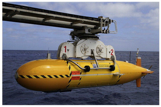
Figure 2.
A specimen of unmanned underwater vehicle (reprinted with permission from [35]).
UUVs are well suited for earth sciences tasks needing unchanged elevation, such as seabed visualization and subbottom profiling, because they can maintain an uninterrupted (linear) trajectory through the water, in contrast to submarine gliders, which are propelled by an inflatable engine and have an undulating trajectory [34]. Although filtering-based methods, such as the Extended Kalman Filter (EKF), provide well-established solutions for irregular issues, their dependence on the linear regression assumption may jeopardize the quality of the results. To overcome this constraint, invariant EKF (IEKF) algorithms based on the idea of smoothing maps have recently surfaced [36]. While inflatable engines allow them to interact in real time and draw more power, from afar, operated vehicles are still connected to the host vessel, which severely restricts their speed, mobility, and geographical range when compared with UUVs [31,32]. When a UUV is in the water, its whole autonomy allows the deploying vessel to be used for other purposes (sometimes even those that are geographically apart from the UUV work area). This greatly increases the volume of information that can be gathered for a particular period of ship time [31,32].
Requiring the use of high-quality video footage, navigational equipment, and sonars, expert human navigators on the surface guide UUV through challenging locations with hot, toxic vent fluids and intricate terrain [31]. Because of the steady energy given by their connections and the high-speed telemetry they receive, UUVs may operate continuously for days [31]. One example of a UUV created especially for scientific research on the deep bottom is the Woods Hole Oceanographic Institution’s Jason UUV. UUVs are widely employed in mapping applications [31]. They are particularly useful for close-quarters, fine-scale sonar, or photographic surveys, where human supervision may enhance safety and efficacy given the tether’s minimal restrictions on vehicle mobility [31]. For larger-scale surveys, UUVs can also yield great findings; however, the vehicle tether restricts speed [31]. Since it isn’t always feasible to add a human touch to all the options in larger elements as well [31], expectations are higher than what our current technology can handle.
Present UUVs for scientific study may function in deeper water of up to 6000 m, contingent upon their pressure resistance (Figure 2) [37,38,39]. The potential for deep-water UUVs to gather seafloor mapping, profiling, and imaging data with a significantly greater spatial resolution (up to a second order of magnitude) and direction accuracy than surface-based vessels and towed instruments, such as side-scan sonar, stems from their ability to fly very close to the seafloor (<5 m altitude in areas of low relief) [38,39]. Thus, UUVs efficiently close the spatial resolution difference between ROV-mounted systems and vessel-mounted or towed systems, such as sidescan sonars (SSSs), subbottom profilers (SBPs), and multibeam echo sounders (MBESs) (Figure 3).
Six levels of vehicle autonomy have been identified by the Office of Naval Research (ONR) [40]:
- (1)
- A system that requires no human intervention when carrying out any of its designed activities is considered fully autonomous.
- (2)
- Mixed initiative refers to an independent framework that permits either the system or a person to respond to data that has been sensed. The system may organize its behavior, both overtly and covertly, with human behavior.
- (3)
- A human-controlled system is capable of carrying out an extensive range of tasks once top-level approval or guidance from a human being is received.
- (4)
- Human-delegated systems are capable of executing restricted control tasks on an assigned foundation.
- (5)
- Human-assisted systems are able to carry out tasks simultaneously with human input. Nevertheless, the system cannot function without supporting human support.
- (6)
- A system that lacks autonomy is referred to as human-operated.
UUVs are also occasionally employed for wireless power transmission in underwater environments. To solve the problem of considerable energy loss in various vehicles during mobile power transfer, an in-depth study based on UUVs using wireless power transfer techniques is required [41]. Through the design of docking devices, adaptive control, and coupling mechanism optimization, the energy degradation during undersea wireless power transmission may be successfully decreased. The difficulties associated with low-loss wireless power transmission for autonomous underwater vehicles, as well as the potential for future research and development areas, serve as a guide for achieving an effective and adaptable energy supply for these vehicles [41].
Diverse sonar infrastructure, laser rangefinders, structured light, and optical odometry are among the sensors that are now in use [42]. None of these numerous sensors are prepared to be developed into controllers that will allow a UUV to quickly adapt to its surroundings changing [42], despite the fact that quite a bit of research is doing just that. Current technology makes it too slow to sense the surroundings or too inefficient to process the data onboard; for these reasons, it is important to research how to create an effective robot vision system for UUVs [43]. Researchers are having difficulty coming up with a novel kind of vehicle that can efficiently build robot vision systems and identify every potential data-collecting avenue [43]. The sensors available today are not good enough to produce underwater robot vision. The amount of time needed to collect and analyze the data is excessive. For a UUV, three knots is regarded as a modest speed [43].

Figure 3.
High-resolution UUV MBES bathymetry of cold-seep structures in the deep-water northern Bay of Mexico (left) and the backscatter mapping (right). (A) abundant heart urchins around the lake margins. (B) while zones of abundant mussels. (C) corresponded to zones of elevated backscatter (dark tones) in the fluid expulsion center to the south. The latter site was also sampled. (D) to investigate orange-stained mud visible on the seafloor (reprinted with permission from [44]).

Since the UUVs must follow a predetermined course or trajectory in many applications, the direction-tracking and path-following difficulties are perhaps the most intriguing and important ones. The main distinction is that a route is independent of time, but a path is parametrized in time. Therefore, in path following, there’s an extra degree of freedom (DOF) in selecting the path attribute and the path-following speed, but in path tracking, the reference location and velocity for a certain time are set [45].
It should be noted that a thorough comprehension of hydrodynamic properties would improve the UUV design, control, and course planning in the deepest oceanic regions. Additionally, a thorough list of the turbulence models utilized in the computer simulations linked to computational fluid dynamics (CFD), hydrodynamics-based geometry improvement, numerical modeling, and drag reduction investigations is included. The best methods for predicting the hydrodynamic variables are the best volatility framework used in computational fluid dynamics and the ideal design of autonomous underwater vehicles based on hydrodynamics [46].
There are several uses of UUVs in dangerous underwater conditions. To be widely used, UUVs must get over a few obstacles. Low-cost underwater communication via wireless technology, durable power sources, sophisticated manufacturing techniques, sophisticated materials, small computer systems on board with powerful computational abilities for improved decision-making, and onboard power production and its effective usage are some of the major obstacles [47].
Recently, the use of PEMFC energy systems for large-class UUVs has drawn the attention of scientists. The study explores the distinct operating difficulties, element requirements, and layout problems that are peculiar to underwater conditions while having not been thoroughly covered in prior years. Furthermore, nations including Canada, Korea, Japan, France, and Germany are creating distinct features for large-class UUVs driven by hydrogen FCES [48].
In order to prevent component failures during functioning, electromagnetic compatibility (EMC) criteria must be adhered to during the manufacture and development stages of UUV power systems. Because of the special underwater setting and the necessity to comply with EMC regulations, incorporating electrical equipment into underwater vehicles is difficult. This kind of vehicle’s efficiency is greatly increased by its good operation, which also keeps other crucial equipment placed in comparable conditions from being disrupted. A thorough grasp of the relevant EMC regulations is becoming more and more important as these vehicles are used in scientific studies, surveillance of the environment, defense, and commercial uses [49].
Supercavitation is also developing in today’s time. In the present research, a compressed air system that can produce supercavitation is used to build a theoretical model for UUVs. Via simulation and theoretical model-solving techniques, the viability of using the compressed air system as the power source is confirmed. Additionally, the main aspects affecting its primary performance are analyzed [50]. Additionally, a comparison between this UUV’s primary functionality and that powered by a lithium battery is conducted. This technology has excellent usage opportunities in comparison with current UUVs. It solves the drawbacks of fuel-based UUVs, including the requirement for oxidant delivery, elevated expenses, and partial combustion [51]. Installing lead–acid batteries in a UUV has significant disadvantages. Lead–acid batteries are quite huge and heavy [52]. They require more time to charge and are nearly impossible to install in larger UUVs than smaller ones [52]. Though we still need to use them appropriately, advancements in fuel cell technology have led to considerably greater efficiency in this specific industry by now [52]. In order to make the fuel cell as efficient as possible for the UUV to operate in the future, scientists are working harder on it [52].
UUVs are used by the offshore survey sector to map the seabed in great detail, which enables oil firms to do maintenance and building [52]. Building undersea constructions in the most economical way and with the least amount of disturbance to the surroundings. Usually, the maintenance task calls for the use of subbottom analysts, substantial visual onboard computing, as well as sensors. The placement of a UUV application entails a region for underwater and mine-detecting applications and replenishment of food, fuel, and weapons [52]. UUVs are used by scientists to investigate the sea and the seafloor employing multibeam, side-scan sonar, INS magnetometers, thermistors, echo sounders, and other underwater sensors, such as water quality sensors and ADCPs [52]. Modern UUVs with their matching maximum speed and depth of operation are seen in Figure 4 [53,54,55,56,57,58,59,60,61,62].
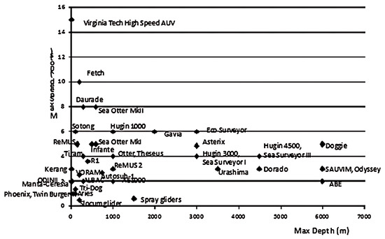
Figure 4.
Unmanned underwater vehicles’ maximum operational speed and altitude (reprinted with permission from [52]).
Recent developments in UUVs may be attributed to several important areas in state-of-the-art underwater robotic technology. Among them are the battery, fuel cells, technology, underwater communication, systems for propulsion, and sensor fusion [52,63]. Important subsystems are categorized into five more broad system categories [52]: mission (world modeling), sensors, computer (SW, HW, fault tolerance), base (hull), propulsion, strength, input fusion, planner, computer work package, emergency, and the sensor for the vehicle directions, navigation, impediment avoidance, communication, self-diagnostic, and support (user interface, simulation, and logistics). As design has evolved, important technological areas have appeared in control, dynamic modeling, and pressure halls/fairings, as well as mechanical systems for manipulators [52]. The continuing investigations are seeking to increase the independence of the underwater vehicle, such as improved designs of increased power density, connectivity, and more dependable deepwater navigation and control action [52].
The main techniques now in use for UUV navigation are inertial navigation and dead reckoning, geophysical systems, and acoustic navigation methods of navigating [33,64,65]. The high cost and electrical consumption of INS and dead reckoning have prevented their widespread usage, particularly for compact UUVs [66,67]. Conversely, INS of lower grades creates an issue with incorrect drift as the vehicle moves with increased separation. An INS integration with additional causes of navigational error-bounding, like Doppler GPS or velocity sonar (DVS) via Kalman [52,68]. It has been demonstrated that filtering is desired as well as a workable resolution. As opposed to the attached ROVs, the UUVs are dependent on the mother ship’s power to function. Electricity is typically supplied by lead–acid batteries. These days, aqueous metal–ion, metal–air, and metal–hydrogen peroxide battery packs, specifically metallic hydrogen peroxide battery packs, have gained popularity because of their oxygen sovereignty, which produces excellent performance while operating in oxygen-free environments like water or space. The energy density of fuel cell technology and fuel cell-like devices is higher, ten to twenty times higher, which has garnered increased interest in the field of UUV strength [63].
2.2. Current Navigation Technologies
The current navigation technologies for UUVs can be divided into three types of sections [15].
2.2.1. Inertial Navigation System
The INS method detects the acceleration of the UUVs using gyroscopic sensors [15]. The first of the biggest scientific and technological challenges is navigating autonomous underwater vehicles. The main challenge is the water media’s opacity against common radiation types, with the exception of acoustic waves. Therefore, the sole instrument for externally measuring the AUV’s attitude and location is an acoustic transducer (array) made of an acoustic sonar. The irregularity of acoustic wave propagation speed, which is influenced by temperature, salinity, and pressure, is another challenge. Therefore, the only way to achieve the required estimate quality and resilience is to fuse the data from the acoustic measurements using data collected by different onboard inertial navigation system sensors [69]. A recent technique proposed by scientists is an analog of the optical flow used in unmanned vehicle video navigation. This technique uses sonar to act as a video camera, creating a picture as a collection of seafloor distances. While the techniques inherent in optical flow require additional refinement and cannot be immediately implemented, this created work will be of great importance in the days ahead [69]. This is frequently used in conjunction with a DVL, which may gauge the vehicle’s relative velocity, and is a major improvement over dead reckoning [15].
While low-cost UUVs can be equipped with inertial navigation systems (INS), high-performance INS can only be found on more expensive UUVs since fiber-optic gyroscope manufacture is challenging [15]. Navigation systems that just employ INS suffer from a progressive loss of location over time because INS accelerometers are prone to drift, particularly if the UUVs maintain a linear trajectory [15]. To enhance efficiency during extended missions, the sea floor’s speed in relation to the UUVs can be determined using a DVL sonar [15]. Comparably, the relative speed of the local current may be determined using an Acoustic Doppler Current Profiler (ADCP) sonar [15]. UUVs can only employ DVL and sonars when they are in close proximity to the bottom of the ocean due to their restricted range. Nonetheless, the location estimate is still susceptible to drift as time goes on when utilizing both DVL and INS [15]. When utilizing a system of that kind for extended missions, it has to find its location in relation to an outside reference point in order to correct any navigational drift [15]. Resurfacing and utilizing a GPS receiver can accomplish this directly, although it is not ideal to do so during deep water surveys, and it is not practicable if the surface is impassable due to ice [15].
In order to prepare for the Atlantic Layer Tracking Experiment (ALTEX), the Monterey Bay Aquarium Research Institute documented the performance of a combined INS and DVL unit with a UUV [70]. The viability of the navigation system for the intended survey was verified, despite issues with calibration encountered with the INS, DVL, and gyrocompass sensors. Utilizing INS, DVL, and ADCP sensors, the Autosub team has also conducted a great deal of study into the functioning of a UUV in ice [71]. Their performance was constrained by the exactness and uniformity of the ADCPs, but they managed to obtain a postprocessed precision that was around 0.2 percent of the assigned distance.
Recently, bio-inspired techniques for underwater location have surfaced. Some characteristics of the light waves remain, enabling more or less trustworthy determination that may be appropriate for navigational purposes, despite early optical technologies not immediately suited for underwater uses owing to the highly rapid capture of electromagnetic radiation in water [69]. The UUV must estimate its location from sensors with extremely varied properties when it combines an INS, DVL, and GPS. Using a KF is a common method of obtaining a location estimate from the sensors [72]. This makes it possible to use GPS fixes to minimize the increasing uncertainty of the location calculation from the INS by giving the GPS signal a constant variance and the INS signal a time-dependent variance [72].
The KF uses a predict–estimate cycle to estimate a system’s state from a series of ambiguous data [15]. First, utilizing an existing physical representation and a mathematical framework that specifies any unknown components, like process noise, a predictive forecast for the future condition and its uncertainty is generated [15]. Then, based on the discrepancy between the forecast and the observation as well as their uncertainties, this prediction is modified using a process observation [15]. A new predicted estimate can be created after this revised estimate has been computed [15].
If the framework is Markovian and linear, and any ambiguities are Gaussian, then the KF is the best Bayesian approximation of the state [73]. In a system like this, the future state is defined as [15] Equation (1).
where represents the physical model and represents the Gaussian uncertainty. This system is characterized by the condition vector and covariance vector at time . Similar to this, ref. [15] the definition of the observation vector is Equation (2).
where denotes the observation process’s physical model and denotes its uncertainty. It is specified that zero-mean Gaussian distributions with the covariances of and , respectively [15], create both vectors, and .
where , and are the updated forecasts, and and are the forecasting estimations of the current condition and covariance vectors [15], respectively, in Equations (3)–(6).
where (Equation (8)) is the covariance of the () term and (Equation (7)) is the Kalman gain. It is evident that based on the disparity between the actual observation and the expected observation , the most recent estimate deviates from the prediction estimate . When the deviation of the prediction is greater than the volatility of the observation , the effect of this disparity depends on the Kalman gain, which is substantial in this case. In this sense, as the findings are more definite, the KF updates the prediction estimations more significantly, which [74] provides a detailed description of a KF appropriate for integration into a UUV navigation system.
Since water absorbs and disperses the majority of electromagnetic signals utilized in terrestrial communications, communication under the sea is severely constrained. This calls for the utilization of acoustic interaction, which is susceptible to interruptions and signal distortion and has a reduced bandwidth. Similar to this, GPS signals cannot pass through water, making navigation more difficult and necessitating the use of sonar and inertial sensors, both of which have chaotic information that will inevitably fluctuate as time passes [75]. It has been demonstrated that the EKF works effectively for steering with an INS and DVL if it receives regular updates from a GPS or another navigational signal. However, in the event that GPS is unavailable, its performance will unavoidably deteriorate [76]. Low-cost sensors will cause this deterioration more quickly, while high-performance INS/DVL sensors can reach 0.01 percent accuracy during short (2.5 km) round missions [77]. Compared with cheaper sensors, this indicates an accuracy gain of an order of magnitude. Statistical linearization is used by the unscented Kalman filter (UKF) instead of the mathematical linearization of the EKF. The unscented transform [78], which resembles a nonlinear function using a collection of points selected systematically to guarantee that higher-order components in the nonlinear function’s Taylor series are approximated, is used in the statistical linearization process. To simulate the higher-order aspects of the underlying uncertainty in this case, more points can be employed [79]. For numerous purposes, especially UUVs, path planning is also crucial. The main challenge is to design and oversee environmentally friendly pathways while using the least amount of energy and money possible. Although the sound-based method was thought to be the primary strategy, there still existed several drawbacks [80]. More recent developments in mobile computing power indicate that a UKF’s higher accuracy for nonlinear systems, rather than its computational efficiency, would be the main driver for its implementation [81]. The issue of inertial navigation can also be solved by particle filters [82]. Nevertheless, these processing needs can be decreased by using novel approaches created for automobiles that alter the number of particles employed in response to the present uncertainty in location [83].
2.2.2. Acoustic Navigation System
The total expense of UUV cluster guidance will rise dramatically with an assortment of submerged acoustic instruments with accurately timed signals, even using conventional acoustic navigation techniques [84]. The UUV may locate itself through the use of acoustic transponder beacons in acoustic navigation [15]. The two most popular techniques for UUV navigation are ultrashort baseline (USBL), which typically utilizes GPS-calibrated transponders aboard a single surface vessel, and long baseline (LBL), which employs at least two transponders spaced widely apart [15]. The UUV is going to navigate the surroundings while carrying out its task, taking routes that enable it to accomplish its goals. A dependable navigating system is necessary to do this [85].
Any technique that makes use of audio beacons that exist in the UUV mission area, irrespective of how they function, is referred to as acoustic navigation here [15]. Although a wide variety of systems have been used, LBL and USBL are the two primary techniques [15]. The range of both techniques is constrained by the size of the transponder network, which is around 4 km for USBL lines in deep water and about 10 km for individual LBLs. Navigation can be facilitated by creating a visual representation of the beacon system using SLAM techniques if the beacon locations are not known beforehand [86]. A stochastic map is required for this kind of map, one that can convey the uncertainty in feature positions resulting from errors in the vehicle’s motion and sensors [86]. The review also refers to CML as the process of figuring out where an autonomous vehicle is located during a mission [87]. It is not necessary to know the beacons’ locations in advance for SLAM methods to create a map based only on observations made of the beacons throughout the mission [87].
Theoretically, autonomous mapping techniques may be used for robot navigation in organized indoor and outdoor areas without the use of artificial landmarks, and they are not just restricted to the usage of artificial beacons [88,89]. Forward-looking multibeam sonar has been used in research where descriptors of particular landmarks are included in the state vector [90]. Although an overall Bayesian structure for recognizing visual landmarks appropriate for SLAM has been put forward [91], the effectiveness of an identical structure in an unstructured submerged atmosphere has not been looked into.
Although mosaics created from side-scan sonar information have been effectively improved by autonomous detection of fake features, the effectiveness of this technique is unknown [92]. A SLAM algorithm continuously determines the precise spot of the vehicle and a related map of its surroundings based on an initial, erratic position and subsequent inspections of beacons. The implementation of such a system is described in detail in [87] using the mapping augmented Kalman filter (MAK) [15] Equation (9).
This enables the implementation of an EKF that can monitor all correlations in one matrix between deviations from the vehicle location and the beacon position [15] Equation (10).
where the off-diagonal vectors , , and represent the vehicle–feature and feature–feature cross-correlations, and is the covariance of the automobile state vector when t = k, is the variance of the beacon vector [93]. The specific CML technique is used to update the augmented matrices and upon the making of a new observation .
The computing demands of a SLAM method might rise as , in which n is the number of points of interest the program uses when vectors such as and are enhanced with more beacons [94]. Utilizing a particle filter and Rao–Blackwell methods, the FastSLAM algorithm decreases the computational cost and achieves , where m is the number of landmarks and n is the number of particles utilized by the filter [95]. It is uncertain how many particles are required to map wider regions. Methods that provide a constant time, complexity increase and converge if the vehicle returns to each small region frequently have been presented [96].
A study on SLAM in an underwater setting was conducted by the Australian Centre for Field Robotics. In [97], SLAM was used to successfully track an array of sonar beacons and determine the precise position of a tethered submersible. A nearby big reef that produced a unique sonar response revealed the SLAM system’s present incapacity to exploit natural cues in practice. Unfortunately, the SLAM algorithm’s navigational performance could not be examined since the vehicle’s location throughout the operation was not externally referenced.
It was shown in a more modern experiment utilizing data obtained from the GOATS ’02 research that a SLAM system could achieve navigation precision equivalent to that attained when beacon positions were known with precision [98]. This implementation employed a voting technique to determine the approximate placements of each beacon and filtering and voting algorithms to eliminate erroneous range estimations. Following this, a state vector supplemented with the beacon placements and the associated covariance matrix was iteratively updated using an EKF.
A detailed performance comparison between an approach that computes all covariances in and the constant time SLAM (CTS) technique is provided in [99]. Leveraging data obtained from the GOATS studies [100], this simulation demonstrated that the CTS method outperformed the traditional technique. However, the algorithm’s association of information was performed by hand, even with the usage of false beacons. The challenge of automatic beacon recognition is unaffected by the CTS algorithm itself, but until this issue is resolved, no such algorithm may be used as an AUV navigation system.
It was successfully demonstrated that an adequate configuration between ASVs and a submerged target can improve the localization precision according to a hypothetical scenario of Gaussian interference. Because of this, the issue is converted into an improved paradigm by applying the D-optimality criteria together with the Monte Carlo approach to obtain the function’s closed-form interpretation [85]. The statistical models that the update filter uses have a significant role in determining the stability and accuracy of such a SLAM system. It could be feasible to destabilize the SLAM method using poorly constructed beginning circumstances, depending on how the system is implemented. By utilizing a set of sub-maps, each cited from a unique, local beacon that contains the most precise, globally referenced position, ref. [96] offers a constant-time approach that avoids this issue. The amount of work required for conventional SLAM techniques grows exponentially with the quantity of beacons employed. An alternate method that lowers computing complexity is to create a sparse matrix of covariance using the data from the form of the EKF [101]. But as ref. [102] demonstrates, imposing sparsity might result in an uneven global map. This is the outcome of the sparsified features’ and the vehicle’s conditional independence assumptions. Using an optical sensor to create a piece of delayed-state information that has precisely sparse yet side-scan sonar is the suggested remedy for this discrepancy. In [97], a tethered submersible successfully tracked and precisely estimated its position using a line of acoustic beacons using SLAM. A big nearby reef that produced a characteristic sonar response served as a demonstration of the SLAM system’s present incapacity to employ natural cues in practice. Regretfully, the vehicle’s position throughout the trip was not externally referenced, making it impossible to assess how well the SLAM algorithm performed in terms of navigation.
This review makes use of information gathered by a Remus UUV [103] while conducting a side-scan sonar ladder search assessment of a section of the sea floor. Since all SLAM algorithms rely on the accurate identification of appropriate features from various vehicle locations, automatic landmark identification is one of the most difficult implementations [103]. As the characteristics of appropriate landmarks differ based on an autonomous vehicle’s sensors and operating environment, suggested approaches are frequently limited to certain scenarios [103]. As naturally occurring underwater characteristics cannot easily be characterized by simple geometric forms, automatic recognition of these features is extremely challenging [103].
2.2.3. Geophysical Navigation System
When a worldwide guidance satellite system is not available, undersea geophysical characteristics might offer significant data for surface navigation. Several submerged characteristics pertaining to terrestrial geophysics can be measured by UUVs fitted with geophysical sensors [104]. This method determines the approximate position of a UUV by utilizing the physical characteristics of its surroundings. These characteristics may be installed on purpose or may already be there [15].
To achieve the best forecast for the vehicle position throughout a mission, the various sensor data from each technique must be analyzed together [15]. Currently, the following methods are employed to estimate the location of the UUV from these data:
- KFs, or Kalman Filters;
- Particle screens;
- Algorithms for contemporaneous mapping and positioning and simultaneous mapping along with localization (SLAM).
Upon superiority, the extended Kalman filter (EKF) is commonly used to jointly estimate unknown model variables and unobserved state variables for stochastic, nonlinear dynamic systems [105]. However, the EKF may become unstable, and the estimates’ accuracy may decline if the equations governing the system’s development contain significant nonlinearities. In this research, we offer an unscented Kalman filtering process and take into consideration recent advances in statistical linearization to improve the results. We demonstrate that the unscented Kalman filter (UKF) performs noticeably better than the EKF in softening solitary degree-of-freedom structural systems when it comes to state tracking and model calibration [106].
Recent research has developed a high-performance method for predicting hydrodynamic coefficients in underwater autonomous vehicles. It is important to use suitable methods to assess and confirm experimental data while modeling an AUV. Hydrodynamic parameter computation is difficult because of the intricacy of the methodologies used for calculation. In order to estimate the hydrodynamic coefficients of an AUV, scientists have proposed analytical methods. The estimation of unknown augmented states (coefficients) is performed using nonlinear Kalman Filter (KF) techniques. The Unscented Kalman Filter (UKF) beats the Extended Kalman Filter (EKF) in terms of performance, according to a comparative analysis [107].
The calculated parameters are compared with the damping coefficient values, which are considered as real values. For hydrodynamic coefficient estimation, the effectiveness of two different recursive state estimation algorithms—UKF and EKF—is investigated. Online estimating techniques are used to estimate the hydrodynamic coefficients, which are supposed to represent an enhanced state in the state space model. According to the results, the UKF coefficient estimate technique has a faster convergence time than the EKF. The UKF estimates these coefficients precisely, despite the fact that the majority of the coefficients predicted by the EKF contain some steady-state errors. As a result, for parameter estimates, the UKF performs better than the EKF [107].
However, OpenSWAP, an inexpensive underwater self-propelled vehicle, is used for geological and geophysical investigations of shallow-water settings. OpenSWAP vehicles can stick to predetermined paths with great precision in suitable climate and water conditions [108]. Certain UUV GPS systems may employ these methods to benefit from their distinct features [15]. Current navigation systems generate a prediction of the UUV’s location and an overview of the positional uncertainty at regular intervals throughout the mission. This information is often presented as a 2D Gaussian distribution. The UUV command system uses this to check if waypoints and other mission goals have been completed [15].
Terrain navigation systems, also known as geophysical navigation systems, estimate the position of a UUV using observable physical elements [15]. This can be accomplished by giving the UUVs an already-existing map of the region or by creating one while the UUV is on a mission. Although approaches for using techniques utilizing local electromagnetic or gravitational changes have been presented [109,110,111], the operational system’s performance has not been documented. Despite a wealth of data suggesting that animals employ comparable mechanisms [112], research in this field has been hindered by the lack of appropriate commercial sensors. Although the combination of various detectors and programmed neural networks has been used to reliably recognize geological features like hydrothermal vents and tidal inlets, such characteristics are rarely seen during a normal UUV voyage [113]. The focus of current research is on using sonar and optical sensors, two types of sensors that are already installed aboard the majority of UUVs, to study physical characteristics.
Due to the weakening of high-frequency electromagnetic frequencies in water, remotely mentioned global navigational aids like GPS are not accessible if the UUV must remain submerged during the operation [15]. Furthermore, it is frequently advantageous from a tactical or financial standpoint to operate a UUV in the absence of surrounding surface boats or acoustic beacons [15]. Certain operations involving mine countermeasures (MCM) and surveys in areas unreachable to surface vehicles require this. The goal of geophysical techniques is to deliver GPS-like navigational performance [15].
Using information from a UUV mission, optical detectors have been studied in combination with automated image registration algorithms [102], and their performance has been reported [102]. Compared with SLAM approaches, registration techniques do not need the explicit categorization of individual features, making them particularly useful in underwater environments [102]. Even though linear mission pathways can yield somewhat better positional results, these approaches work best for missions in which the UUV travels to a recently visited location so that any positional errors resulting from detector drift can be corrected back to initial values [102]. Within a limited range, underwater cameras can serve as dependable, high-quality sensors; any UUV that relies on optical sensors for navigation must function in close proximity to the ocean floor [102]. UUVs used to track seafloor features are not affected by this. Optical approaches, however, need careful lighting, and many of the commercial UUVs already in use are difficult to alter to produce appropriate light sources [102].
An alternative SLAM system with a camera and an augmented-state Kalman filter for automated identification of previously visited regions is described [114]. A mosaic of the camera data collected during the trip is created to determine when the UUV crosses over its mission route [114]. The augmented state Kalman filter (ASKF) is applied as a filter to smooth out the prior position estimates after detecting a crossing. When the UUV approaches a previously visited location, the ASKF [114] may then rectify the UUV’s completely predicted mission route. During a UUV mission, this can be used to verify that the mission goals have been completed [114]. This system’s performance was evaluated with a UUV simulator designed specifically for the [114] GARBI UUV. The capacity of the patchwork system to identify previously visited places using actual UUV mission data—which may contain considerable biases—was not tested in the simulation, though [114].
Even if there are still issues with automatically identifying naturally occurring underwater features, it will be hard to put into practice a trustworthy, ref. [15]-based features, autonomous mapping system. Nonetheless [15], UUV navigation might benefit from the usage of current maps of a region. Underwater feature recognition is made easier when utilizing an existing map since the features’ location and description are known [15]. Survey missions, which are frequently conducted in regions that hadn’t been historically surveyed, are not well served by this strategy [15]. Nonetheless, a present map will frequently be accessible if a UUV has to navigate accurately in a familiar location, such as the vicinity of a harbor [15].
UUV navigation has been extensively investigated with high-detail terrain images of specific regions produced by multibeam sonar studies [115]. It has been demonstrated that a UUV’s position may be determined to be inside a few meters while it is inside one of these zones by using a maximum-likelihood technique in conjunction with a multibeam sonar [116]. Because the system calculates for more than 80 distinct sonar beams, the approach has significant computing needs; however, these expectations may be satisfied by designing the mechanism as a field-programmable gate array (FPGA) [117].
By importing an existing map with appropriate feature positions and covariances, SLAM algorithms can leverage it to enhance navigation performance [117]. However, existing SLAM algorithms demand a single, recognizable point, which makes it difficult to identify genuinely occurring underwater elements [117]. To make the most use of geophysical maps, this indicates that a significant revision of existing SLAM methods is required unless a mechanism is discovered for representing underwater characteristics in this manner [117].
Using current maps, filtering particles have been studied for navigation [83]. In theory, geophysical sensors may offer predictions of the vehicle’s location, heading, and velocity through the use of particle filters [83]; however, if the heading and velocity of the vehicle are provided by the UUV’s current sensors, the filter’s complexity can be reduced. Using current maps, filtering particles have been studied for navigation [83]. It takes time for a particle filter to stabilize if it is initially filled with a large dispersion of particles [118]. This is not an issue for UUV navigation, though, because missions undertaken by UUVs that are deployed from surface vehicles may obtain an initial, GPS-referenced location [118].
The current UUV location estimate is computed using all the particles and weights [118]. A tiny percentage of the elements will have big weights, whereas numerous particle weights may approach zero as additional updates are performed [118]. The term “degeneracy” refers to this process, which is especially significant when the physical process has little noise [118]. Because fewer particles may be utilized to determine the state efficiently due to degeneracy, the calculated value of the state is less accurate [118].
Underwater navigation has been studied with particle filters in conjunction with elevation maps, and simulations indicate that this is a practical strategy [119,120]. This technique has a big benefit in that the filter doesn’t need to explicitly classify different undersea elements [119,120]. The symmetries on the on-board map result in estimations of the UUV’s position that are frequently multimodal [119,120], which makes the particle filter able to describe the vehicle’s location more precisely than a parametrized distribution [119,120]. However, because the efficacy of the particle filter is sensitive to the degree of noise present, the methods employed heavily rely on the preciseness of the detectors and the map [119,120].
The estimation of the UUV’s location is successfully discretized by using a particle filter. A point-mass filter is an older, different technique that discretizes the estimate as well [121]. On the other hand, the application of a particle filter permits the separation of linear components of the estimating process from the estimation issue using established techniques like Rao–Blackwellization and permits the incorporation of new sensor information without substantially altering the system [121]. The Rao–Blackwellization technique uses KFS to estimate the components of the state vector that can be described by linear, Gaussian processes [121]. This approach requires significantly less computation because the integrations necessary to calculate the updated components can be performed analytically [121]. A Rao–Blackwellized approach has been implemented, and its performance has been tested on a simulation using an elevation map from survey data [120].
Using an appropriate distribution at time k, a particle filter generates an enormous number N of state estimates (referred to as particles) along with weights in order to maintain an accurate estimate of the AUV’s location. The particles and their respective weights have been updated employing sequential importance sampling (SIS) at the time of observation . A particle filter takes longer to stabilize if it begins with a large dispersion of particles [118]. Nonetheless, this is not an issue for AUV navigation because surface-based AUV missions may be given a starting, GPS-referenced position.
A re-sampling particle filter uses a starting likelihood density function of the state vector to produce a significant amount of particles and their corresponding weights . The significance density is estimated at time k using the observation . Using the importance density and SIS, it produces N new particles with their weights . The efficient sample size is estimated using = 1/. Use the statistic to re-sample a fresh set of particles with the same weights in addition to the existing weights if , where is the threshold value. Specific particle filters are discussed in greater depth in [122]. The computation of novel particles for geophysical navigation must be based on the variation of an observable physical property in the vector and the value of that attribute on the on-board map of the AUV. The local variance of will have a significant impact on the overall distribution of the significance density that was previously described. Particles will start to become more scattered, and their significance density will be homogeneous in regions where varies slightly.
In its most basic version, the particle filter approach has very high computing needs [120,123], even if its Monte Carlo methodology seems easier to apply than the analytical demands of the KF and SLAM methods when traveling from an existing map [120,123]. Implementation becomes more challenging if methods to decrease the computation are employed, such as Rao–Blackwellization or variable frequency particle filters [120,123]. Selecting the appropriate significance density for filter updates is crucial for non-Gaussian signals and can be challenging to determine [124]. Generally, UUVs are utilized in large-scale exploration scenarios, and because of their small size, they may be readily buried extremely deep in the water for more thorough research.
2.3. Present Challenges
2.3.1. A Framework for Using Sonar Navigation with Existing Systems
Sonar is a major data-collecting tool for UUVs nowadays; however, there is a methodical approach to utilizing sonar systems to facilitate navigation [125,126]. Although the use of particle filters and SLAM to aid in navigation during a UUV mission has been suggested, no formalized procedure for doing so has been devised [15,126]. Aquaculture parameters related to water quality may be monitored in line with established paths based on the AUV’s multi-parameter liquid quality sensors parallel with SLAM. To do this, the UUV’s location in relation to its net pen must be estimated during its inspection [126]. While a KF may be used to merge INS and GPS, sonar-based navigation systems should not employ this method as their estimations do not adhere to a Gaussian distribution [125]. These technologies cannot be employed to enhance the navigating performance of current UUVs without an infrastructure for integrating their estimations with those of already-existing systems like INS or USBL [15]. Consequently, many studies have looked into postprocessing mission data using statistical approaches [15,126], but none have shown how well such a system works when it is incorporated into a UUV and utilized during a simulated trip [15].
2.3.2. Navigationally Optimal Routes
UUVs must follow a course established by the operator, which is typically referred to as a waypoint system, in order to fulfill the mission criteria of contemporary academic and commercial UUV operations [15,127]. Autonomous mission control UUVs are limited to rules for breakdowns in systems and collision avoidance. UUVs need to have the ability to depart from a user-defined course to accomplish their mission objectives, especially if they are to be utilized for more difficult tasks like intelligent surveys, port defense, surveillance, or MCM [15,128]. A more advanced navigation system that is capable of estimating its effectiveness for a specific mission path is needed for these missions [127]. Extended resilience AUVs can enable more difficult mission types than are now feasible. One important technique for extending AUVs’ lifespans beyond what batteries can provide is using fuel cell technology. Yet operating fuel cell devices underwater presents a number of difficulties. These have to do with buoyancy and reduction, the demanding conditions of the surrounding saltwater, and the creation or preservation of hydrogen and oxygen. There are additional difficulties with water retention, cooling, and the buildup of inert gases or reactants when the fuel cell is protected inside an airtight container [127]. A UUV may try to follow a route without a system like this, which would cause a significant loss in navigational accuracy. The literature does not address the assessment of future performance for any UUV positioning system in a particular circumstance [127].
2.3.3. Relative Placement and Reactive Control Using Local Characteristics
UUV missions will increasingly need to route locations concerning underwater structures like harbor walls or pipelines [128,129]. Although UUV navigation systems can monitor their surroundings extensively, employing side-scan and multibeam sonars, they are unable to employ descriptions of those surroundings for relative control [129]. Machine vision technologies are available for optical sensors. Each UUV component (hull and structural components, driving and electrical system, GNC, telemetry, payloads, information management, and ground station) has advanced significantly in recent years, following an evidently experimental starting point with limited options in terms of independence, endurance, payload, energy outputs, etc. Even so, they haven’t been completely optimized lately [129]. Because surface vessels are more constrained by surface weather conditions, operating from a harbor offers lower operating costs and more operational flexibility. Effective frequent patrols will require this manner of operation if UUVs are going to be utilized for port defense [127,128].
2.3.4. Navigating with Little Sonar Use
While few research missions are interested in the topic, many military applications need minimum sonar usage for navigation. While optical sensors, laser scanners [125,130], and passive sonar arrays are viable options, their dependability and range are constrained, necessitating the UUV to operate in close proximity to the ocean floor [125]. Finding the least amount of sonar use required to accomplish a given mission’s level of precision calls for a complex solution that isn’t currently covered in the literature [15,127,130]. The current navigation technique is to employ a high-quality INS in conjunction with an occasional DVL when limited sonar utilization is necessary [15,127,130]. Since this system is an open loop, drift will unavoidably occur during the flight, reducing the UUV’s range. The challenge therefore becomes limiting map consumption while decreasing positional inaccuracy if a topographical map is utilized [15]. A graph-theoretic analysis of the mission’s path and map, as well as an assessment of the most information that can be obtained from the visualization along a certain path, would be required to solve such a task [125,127].
2.3.5. Navigating with Significant Features
Future missions involving close contact with obstructions like docks, pipelines, and manned vehicles are anticipated to employ UUVs [131]. UUVs will need more modern navigation systems in addition to more complex control systems to carry out these tasks [131]. The system to navigate must be able to use image sensors, such as webcams and side-scan sonars, to offer more precise information about adjacent objects to apply instructions necessary for effective operation near these impediments [131]. There is no system in place for organizing the bigger, more planned elements that are probably to be encountered in a busy transporting environment, despite methods having been proposed to extract distinctive characteristics from tiny characteristics and research on the categorization of mine-like underwater things being conducted [131]. It seems doubtful that techniques like side-scan image comparisons, which are produced from models designed for tiny objects, will be effective for bigger features. The UUV’s relative location has a significant impact on the appearance of huge underwater objects [132]. Instead of doing a straight visual study, this recommends a 3D method [132]. On the other hand, it can be challenging to extrapolate 3D information from traditional side-scan sonar data and needs to make assumptions about the environment’s acoustic properties and reflectivity [132].
4. Underwater Navigation Sensors
The envisioned underwater navigation system’s primary components are the IMU, DVL, and USBL. The installation architecture and data computation of these components are crucial to the system’s operation.
4.1. Inertial Measurement Unit (IMU)
The most important sensor in the UUV is the IMU, and the sensor’s accuracy, precision, and stability may all be increased in a number of ways. To lower the IMU’s noise measurements, for example, testing the positioning of the module in an area with less magnetic interference or utilizing various kinds of filters is applied [144]. Additionally, an innovative approach to IMU fault estimation has been developed recently to identify IMU faults and achieve IMU signal reconstruction [145]. When compared with fiber optic gyroscopes, Micro-electro Mechanical Systems (MEMS) IMUs provide notable benefits in terms of power consumption, weight, and volume.
Auxiliary magnetometers, which have a precision level similar to a fiber optic gyroscope, are a feature of certain MEMS IMUs [146]. Certain commercial MEMS IMUs may incorporate magnetic data that generate the directional angle in addition to providing the angular velocity and linear acceleration, which considerably increases accuracy and convenience [146]. Linear complementary processing can be used to determine the attitude of certain MEMS IMUs that are unable to do so directly [146]. Three-axis accelerometers and three-axis magnetometers can be used to determine the stable attitude angle without a cumulative mistake [146].
4.2. Doppler Velocity Log (DVL)
For more than ten years, DVLs have been gaining popularity as navigational aids on ROVs, UUVs, and even human-occupied vehicles. In modern times [147], DVL is the most advanced and accurate velocity navigation device for underwater vehicles. It has different characteristics when tracking the velocity of the movement of underwater vehicles [147]. Although it’s very costly, the DVL comparatively gives much higher accuracy compared with the other velocity sensors [147]. When bottom tracking velocity readings are obtained using acoustic measurements, DVLs can offer updated velocities that can be utilized to compute distance traveled. Traditionally, only bigger trucks and boats with the cargo capacity and data bandwidth to transport the subsea acoustic arrays have been able to deploy DVLs [147]. A recent development by several manufacturers is an emerging category of shorter DVLs that exhibit identical performance attributes to their bigger siblings despite a significant size reduction. As shown in Figure 5, DVL often uses a four-beam Janus design for measuring velocity. This entails setting up the two transducers for each of the four directions before and following the DVL [147], which can significantly reduce the inaccuracies brought on by the front and back of the carrier wobbling.
In the past, DVLs were devices that could only be carried by big underwater vehicles, manned submersibles, and work-class UUVs [147]. These vehicles possess the payload capacity for transporting a DVL in addition to the other instruments and equipment required for their missions. A 3000 m rated DVL typically weighs more than 8 kg when submerged and more than 15 kg in the air [147]. Bigger submersible UUVs and human submersibles are needed to deploy even smaller DVLs that are rated to shorter depths since they weigh more than 9 kg in the air and more than 4.2 kg on land [147]. Sometimes, DVL-denied settings and DVL errors or fallacies can occasionally appear as unanticipated reasons for serious positioning system faults [148]. The model-based method may be replaced with BeamsNet, a complete deep-learning platform that regresses the predicted DVL vector’s velocity to increase its accuracy. Different iterations of BeamsNet are proposed, with different inputs to the network. While the other uses simply DVL data, using both the current and previous DVL readings for the statistical regression procedure, the first uses both the inertial sensor information and the current DVL beam readings [149]. The issue that systematic flaws have a significant impact on irregular terrain as well as are challenging to detect is resolved by using a dead reckoning framework to identify the overall residual and adjust for DVL terrain-assisted navigation, which is based on the consistency principle of sensor hardware [150]. The DVL sensor provides high accuracy in measuring the velocity data for any kind of autonomous underwater vehicle [147].

Figure 5.
DVL velocity measurement schematic diagram (reprinted with permission from [151]).
Figure 5.
DVL velocity measurement schematic diagram (reprinted with permission from [151]).

Doppler velocity measurements are essential for improving underwater vehicle performance and accuracy, especially when combined with Doppler Velocity Logs (DVLs) [152]. These systems are used in a variety of situations, guaranteeing efficient data collection and navigation in submerged settings. Because Doppler velocity measurements give accurate estimations of the vehicle’s velocity in relation to the bottom, they are essential for subsea navigation [153]. This feature is crucial for navigation in situations when Global Navigation Satellite Systems (GNSS) are not accessible, including deep-sea missions or beneath thick water columns. Underwater vehicles can carry out intricate activities like mapping and surveying because of the information generated by DVLs, which includes immediate velocity and positioning data [149].
Underwater vehicles can gather important environmental data through Doppler velocity measurements, which can be utilized in oceanographic and scientific research. Conditions including bottom topography, water currents, and environmental elements impacting marine ecosystems may all be evaluated using DVLs [154]. The knowledge of the underwater realm is improved by this capacity, which enables missions ranging from ecological monitoring to undersea structural inspections. It also makes a substantial contribution to underwater vehicle obstacle avoidance techniques. By supporting real-time evaluations of the vehicle’s environment, these metrics aid in collision avoidance [155]. Vehicles can improve operating safety in challenging underwater settings by identifying possible risks and modifying their routes in response by combining DVL data by adding sensors [149].
Nevertheless, the observer has a direction finder that assesses the target’s azimuth, elevation, and range in order to estimate the target’s coordinates and velocity [156]. Because of the nonlinearity of measurements, nonlinear filters are typically used to alleviate such issues. However, in the lack of accuracy estimates, the majority of filters provide estimates with unknown bias. The target’s unobservability is a significant issue [157]. To convert the estimation issue into a linear problem, a pseudo-measurement technique is suggested. With this method, the unobservability issue may be resolved, and the position and velocity of an evolving objective can be estimated. Computer simulation results demonstrate the effectiveness of the suggested approach in solving the passive target tracking problem [158].
4.3. Ultra-Short Baseline (USBL)
Ultra-Short BaseLine (USBL) acoustic technology is a viable means of correctly detecting the position of UUVs in relation to surface boats, which is a critical need for operational, safety, and budgetary reasons. In consideration of the foregoing, numerous acoustic location techniques have been created in the past. See, for example, the highly effective systems © Ranger 2 and © GAPS [159], as well as the USBL locating system known as POSIDONIA [160]. Though smaller than their predecessors, the Easytrak USBL systems from ® Acoustics [161] and the R-Series USBL [162] from ® nonetheless provide effective solutions for a variety of subsea applications. The USBL system achieves the positioning function by calculating the relative position between the carrier and the transponder [163]. The positioning system for the USBL uses a transmitter to transmit a fixed-frequency acoustic signal to a transponder at a known location on the seabed [163].
Basically, the USBL-based method used a UUV to attach the sensor and function as an alliance to help the underwater robot’s navigation, whereas the DVL-based guidance technique used conventional dead reckoning to navigate [164]. The system determines the tilt distance based on the time difference between the transmitted signal and the received signal and the azimuth angle based on the phase difference between the received signal and different hydrophones to achieve the positioning information for UUVs [163]. The three hydrophones are arranged on two perpendicular baselines (the x and y axes), as depicted in Figure 6. Eustice et al. [65] described recent developments in underwater navigation that rely on synchronized one-way travel periods of acoustic waves, which are accessible via expensive higher precision oscillators [165,166].
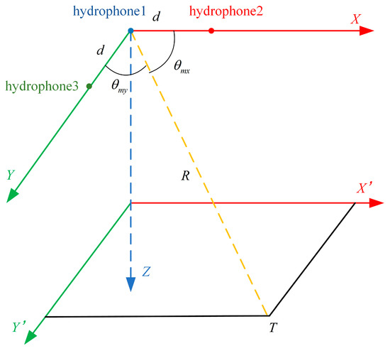
Figure 6.
The USBL positioning measurement schematic illustration (reprinted with permission from [151]).
Furthermore, inverted USBL configurations enable sound speed to be regarded as constant while functioning in the same underwater layer by layer as the transponders [165,166] (e.g., bottom operation while investigating a bottom-placed transponder), opening the door for future fully autonomous vehicles that do not require surface purpose support vessels. Other underwater autonomous regular tasks [165,166], such as underwater interventions and localization and docking to underwater stations, are also made possible by these types of inverted setups [165,166]. A tightly linked USBL/Dead Reckoning (DR) combined localization technique that takes into account the time-varying properties of the measurement error should be utilized in order to increase the positioning reliability of the USBL-based incorporated navigation system [167,168].
4.4. Equipment Configuration and Frame Specifications
The explosive properties of torpedoes are always being enhanced [169]. For neither, a towed or disposable noisemaker continues to be the main line of defense as of right now using an inflatable generator, which creates a substantial cloud of bubbles by a chemical reaction to function as a misleading target [169], continuing to be the major defense against submarines. Figure 7 displays the arrangement of pertinent apparatus as well as the definition of two reference frames [169]. In this two-dimensional body, several specifications are marked for the better conceptualization of the UUV’s characteristics. There are pitch, sway, yaw, and heave, along with roll and surge, displayed in the body for better understanding. The USBL is fitted at the nose of the body here.
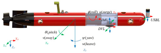
Figure 7.
UUV layout (reprinted with permission from [151]).
The body frame lies in the position of the center of gravity of the UUV, with the X-axis leading in the direction of the vehicle’s forward motion, the Z-axis pointing down, and the Y-axis completing a right-handed regard frame [170]. The navigation frame originates on the outermost layer, and its axes point North, East, and Down [170].
5. Types of Velocity Sensors for UUVs
5.1. Ultrasonic Speed Sensor
The ultrasonic sensor gathers echoes from tiny water particles as they pass beneath two transducers set into the insert using ultrasonic pulses (Figure 8) [157,171]. These transducers keep an eye on the particles within the beams they are assigned. Both transducers see an identical stream of particles as the UUV moves through the water [171,172]. The sensor detects the smallest particles later than the force transducer, as it takes time for nanoparticles to move between the two transducers. The device determines the UUV speed by calculating this time-lapse [171,173]. Water-suspended particles and other contaminants have a significant impact on the sensors’ accuracy; in muddy and aerated environments [157,171,172], the sensors will estimate the speed incorrectly. Special installation requirements also apply, such as the need to mount the device in an area free of water bubbles and fluid flow turbulence. According to studies [157,171,174], an ultrasonic axial speed sensor is employed for a UUV’s inexpensive inertial navigation.
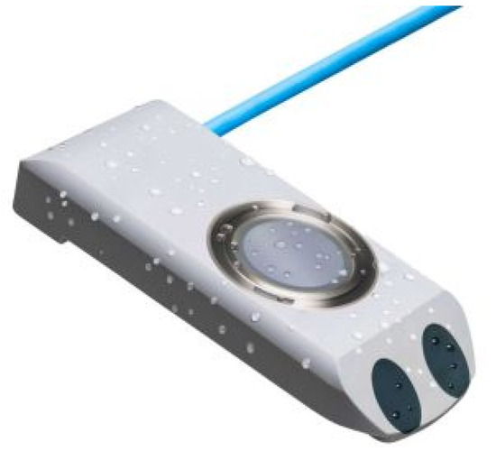
Figure 8.
A simple ultrasonic speed sensor (adopted from [175]).
The general specifications of a simple ultrasonic speed sensor have the following characteristics (Table 2).
Table 2.
Ultrasonic speed sensor characteristics.
5.2. Paddlewheel Speed Sensor
The turbine (paddlewheel) speed sensor (meter) is a kind of flow metering device that is frequently used to measure liquid flow rates [178,179,180]. It is frequently chosen over substitutes in many engineering applications because it has the benefits of being relatively easy to install and operate, being robust, and having sufficient precision for these instruments’ [178] typical applications in the recording of commercials for different drinks. An account of the very first turbine flow meter dates back to 1938. Several turbine flow sensors [179,181,182,183] have been developed in recent decades to measure the flow rate. Numerous researchers have made significant progress using turbine flow sensors [179,181,182,183]. Conventional turbine flow sensors feature several disadvantages, including being large, expensive to manufacture, and susceptible to electromagnetic fields readily contained by the material of turbine blades (Figure 9). Fiber optic flow sensors provide several important benefits over typical turbine flow sensors (electronic and MEMS sensors) [180,184], including being simple to use, having a high sensitivity, having a long lifespan, and being resistant to electromagnetic fields—remote sensors, and so forth [180]. Flow-rate measuring with optical fiber instruments has been more popular recently. This is observed based on the turbine’s blades varying the intensity of the reflected light [184], significant The field of optical fiber flow sensors has advanced. However, the majority of them are challenging in real life as well as their applicability because of the expensive and sophisticated measurement methods and their infancy [184,185].
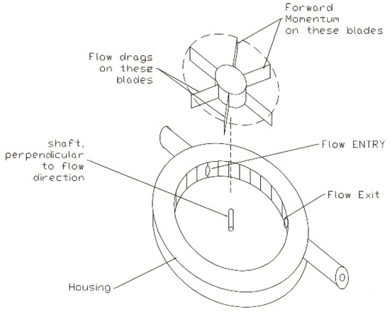
Figure 9.
A small (paddlewheel) speed sensor (reprinted with permission from [186]).
The basic specifications of a sample paddlewheel sensor have the following characteristics (Table 3).
Table 3.
Paddlewheel speed sensor characteristics.
5.3. Doppler Velocity Log (DVL) Sensor
UUVs have a difficult navigation challenge due to the low propagation lengths of radio frequency signals, like GPS [148,188], in water. Periodically, surface UUVs can obtain a GPS fix, but it’s preferable to keep the mission continuing without interfering [188]. Most UUVs that need high-fidelity navigation employ one of two techniques in between GPS fixes: positioning using acoustic transponders or using INS with the help of a DVL [148,188] (Figure 10). Installing and maintaining these navigation solutions can be expensive and time-consuming. Thus, in cost-sensitive applications, lower-fidelity navigation techniques like terrain or propeller-count assistance of MEMS INS are occasionally used [189,190]. The basic quantity that an INS monitors directly is acceleration, which is double integrated to determine position. By sending out several beams of acoustic pulses that reflect off the bottom [190], a Doppler velocity log calculates the difference in speed between the sensor and the water’s surface. Four beams spaced 90 degrees apart in azimuth and raised from perpendicular by an ordinary angle known as the Janus angle make up a typical design [189,190]. After receiving the dispersed sound, each beam’s radial Doppler shift is determined using [190] Equation (11).
where is beam I’s radial velocity, c is the speed of sound, is the received frequency, and is the frequency at which it is transmitted [191]. Eliminating squared Mach number terms—which are minimal for average velocities—gets us to the approximation [188]. Transforming the calculated radial Doppler shifts of the acoustic rays into instrument coordinates yields a three-dimensional velocity vector for each ping [188]. A speed scale-factor error or bias causes a DVL to measure velocity directly, needing just one integration to determine position. This leads to a linear development in the positional error over time, as opposed to a quadratic one [8]. In the past several decades, there has been a significant increase in the development and use of especially UUVs and AUVs [8]. Four-beam DVLs are typically utilized in multibeam DVLs [155].
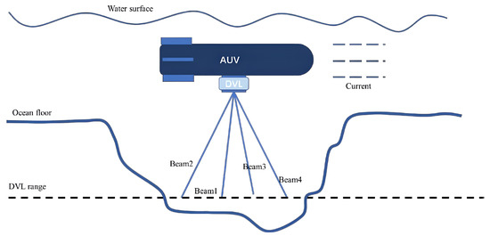
Figure 10.
Doppler velocity log (DVL) sensor working process (reprinted with permission from [192]).
Even though high-end INS may achieve dynamic accuracy of up to 0.1 degrees, their considerable cost can often compel users to adopt less expensive [193] MEMS AHRS (Attitude Heading Reference System) for less important applications [193]. A technique for estimating the optimal attitude (roll, pitch, and yaw) utilizing the gyroscope, accelerometer, and magnetometer data in the AHRS is necessary in order to use the MEMS AHRS [193]. The majority of autonomous vehicles are designed to swim in a predetermined region and pattern [193]; they have no ability to “see” where they are heading. In order to confirm its location and proceed on its pre-programmed route, the UUV will make use of onboard sensors like the Doppler Velocity Log, Global Positioning System, or Inertial Measurement Unit [193]. It may become lost or become stuck if a new object comes to cross its route or if it veers from the intended path [193]. Therefore, for DVL navigation, the estimated attitude estimates are employed [193]. By contrasting the DVL guidance trajectory with the established ground truth trajectory, the attitude assessment performance is therefore assessed indirectly [193].
The most recent development in UUV technology is downsizing; several manufacturers now provide man-portable vehicles [190], which enable quick and inexpensive deployments in shallow water. Fitting inside the 36-inch-long, 4-inch-diameter cylinder of an A-size sonobuoy is a common size restriction for AUVs [190]. The micro-UUV is also appropriate for use cases that call for an inexpensive or disposable UUV, such as multi-vehicle missions [190]. Due to size and budget constraints, these vehicles may employ alternative lower-fidelity navigation techniques depending on the mission; however, they do have limited payload capacity and benefit from INS- and DVL-based navigation [190]. The vehicle’s linear velocity within the vehicle coordinate reference is provided by the DVL sensor. The below equations translate the linear velocity in the vehicle reference frame towards the linear velocity in the global coordinating frame [190].
where R is
Here, , and
The straight-line velocity in the world reference frame is denoted by in Equations (12) and (13) [190], whereas the linear velocity in the motor vehicle coordinate frame, as determined by the DVL, is represented by . The position of the vehicle is obtained by integrating the velocity [190].
DVL sensors have many unique specifications; among them, some are mentioned below (Table 4).
Table 4.
Doppler velocity sensor characteristics.
5.4. Optical Velocity Sensor
Since high-quality photos and video are essential to the majority of ocean scientific studies [195,196], research UUVs are often equipped with broadcast-quality cameras and high-output lighting systems. This creates ideal circumstances for us to employ vision for accurate underwater robot navigation and placement [196]. Additionally, this aligns with several academics and business experts [196]. If we consider applications on land, for example, self-driving automobiles and aerial drones use computer vision and image sensors to solve similar difficulties, which serve as inspiration with precise navigational aids [195,196]. Through identifying contextual elements, the platform’s relative position may be monitored while mapping the actual surroundings at the same time observed [196]. In addition, vision may be used in tandem with various sensors to provide more thorough and reliable navigation and placement [196]. For these reasons, following the development of profound learning, after a period of stasis, UUV underwater navigation dependent on vision may give better information, cheaper pricing, smaller sensor sizes, and reduced energy consumption. In both scientific and industrial circles, it has grown to be a center for study [197,198,199,200]. However, vision is a passive form of perception that might lessen its influence on the delicate ecological environment [201]. Underwater optical navigation and location is a potential technique that can yield outstanding results, particularly in coastal areas with clear water and adequate illumination (visible up to 20 m) [201].
A series of compact, standalone, laser-based optical velocity sensors makes it feasible to monitor surface and underwater vehicle speeds accurately in relation to the surrounding water [202,203]. Diffractive optical elements (DOEs) have allowed for the downsizing of sensors. A “time-of-flight” micro-velocimeter is the type of sensor used in this book to measure the speed of a vessel with the water surrounding it [202,203]. Additional sensors created by MSE include the wall shear stress monitoring ™ and the remote velocity measurement ™. The references section contains papers [202,203] that describe these sensors in Figure 11.
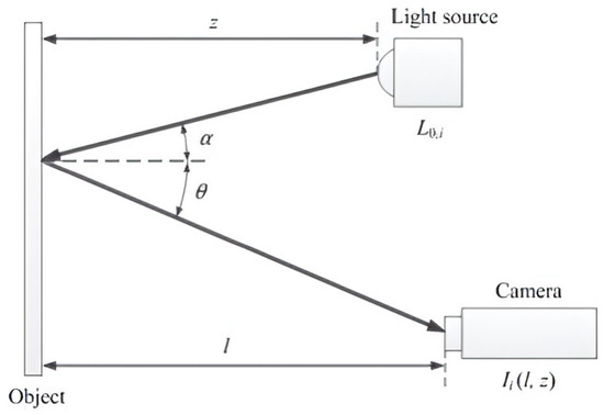
Figure 11.
Optical velocity sensor working principle (reprinted with permission from [204]).
A compact and durable velocity sensor known as ™ [202,203] has been created to measure the instantaneous velocity of minute particles in the water concerning the vessel, allowing for a direct assessment of the velocity of both surface and underwater vessels [202,203]. The transmitting and receiving optics are combined into only one diffractive optical element (DOE) to form the sensor. A laser light source shines two parallel light strips at a distance of 10 mm (7.5 mm in the air) [202,203] from the sensor’s surface to highlight the doe. Two light sheets with 5 μm thickness are apart from 100 μm and display a picture of how the light reflects in the liquid [202,203].
It has employed a variant of the soft-operator iterative-Fourier transform technique [202,203] to create the doe as a beam-shaping generated by the software hologram phase function. The primary option for autonomous location and surroundings perception lacking previous awareness of the surroundings and external supplemental information sources is vision-only approaches, which solely realize placement through photographs [202,203]. Combining vision cameras with additional sensors, such as depth meters, sonar, and inertial navigation, allows vision-based multi-sensor fusion techniques to provide more reliable and precise video-based localization (vSLAM) [202,203]. Figure 12 shows the geometry-based optical navigation system [202,203].
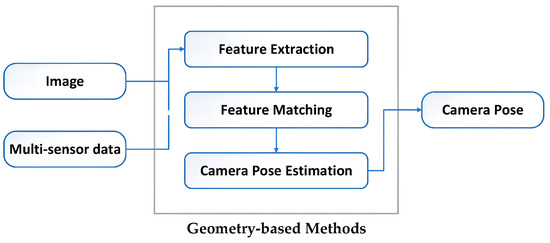
Figure 12.
Visual navigation system layout (reprinted with permission from [12]).
The two primary types of traditional geometry-based vSLAM techniques are feature-based and direct vSLAM techniques. By comparing feature descriptors [205], the feature-based vSLAM approach primarily finds feature points in neighboring pictures and matches them. It then resolves the camera posture based on the matching connection [205]. For a considerable amount of time, enhanced Kalman filter (EKF) SLAM, one of the feature-based vSLAM techniques, dominated the early field [206,207]. The initially developed real-time mono vSLAM system was called MonoSLAM [208]. It tracked sparse points of interest at the front end using EKF to operate the back end and updated the camera posture and mapping frame by frame using a single thread. The issue is that even at the lowest levels of complexity [208], the computing cost rises in direct proportion to the dimension of the environment. The use of vSLAM was significantly constrained by FastSLAM [95]. A significant advancement in the realm of vSLAM, PTAM was introduced by [209] in 2007 and creatively suggested a dual-thread framework for surveillance and mapping [209].
Although the mapping thread had longer processing times since it did not need to be adjusted frame by frame, the location tracking thread was utilized to alter the camera posture in real time. As a result, vSLAM [209] additionally uses the combination adjustment technique, which was previously limited to offline architecture from motion. Since then, this multi-threaded architecture has been used by nearly all vSLAM algorithms [209]. While the projection thread had longer processing times since it did not need to be adjusted frame by frame, the monitoring thread was utilized for modifying the camera posture in real time [209]. As a result, vSLAM additionally uses the bundle adaptation (BA) technique, which was previously limited to offline shape from motion (SfM) [209]. Since then, this multi-threaded design has become the standard for practically all vSLAM algorithms. The three-thread structure of ORB-SLAM2 [210]—tracking, local mapping, and loop closure—achieved extremely strong monitoring and mapping visuals, which can guarantee the worldwide consistency of the map and the trajectory—following the two-thread framework of PTAM [211]. In addition to ORB-SLAM, the monocular version was called ORB-SLAM2 [211]. It served as an example of feature-based vSLAM techniques and supported RGB-D, monocular, and binocular cameras [211].
A 500 mm solid quartz substrate was used for single-sided lithography to create the ™ [212] sensor components. The acetone development process was used after analog direct-write electron-beam lithography to create polymethyl methacrylate (PMMA) diffractive lenses [212].
Light is scattered by tiny particles moving through each light sheet, collecting onto receiving optics built within the sensor [212]. The ™ [212] sensor is permanently embedded in a tiny stainless-steel housing, so it never has to be adjusted. The detector is calibrated at production, thus the user does not need to do any extra calibrations. ™ [212] is insensitive to changes in ocean water temperature, salinity, or pressure because of its linear response. Figure 13 shows a completely assembled sensor [212]. The sensor can be installed flush with the vessel wall to prevent disruption of the flow, or it can be used as a standalone, waterproof sensor that can be inserted into the flow [212].
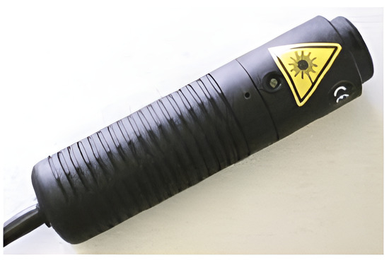
Figure 13.
An optical speed sensor (adopted from [213]).
The flow conditions in which the ™ was actually employed are diverse [214]. The sensor’s analog output for one particle traveling via every one of the two beams is almost identical. By using the measured time-of-flight [214] and the physical spacing between the two fringes, one may determine the particle’s speed. The flow’s instantaneous speed is directly proportional to the measured [214]. The environment’s information richness can be enhanced by the addition of an IMU, enabling high-frequency, robust, short-term, exact placement under challenging conditions for vision cameras [214], like texture-missing and picture blur.
However, the fused vSLAM technique may achieve greater accuracy and resilience because the vision technology can address the cumulative mistake and large drift of the IMU [214]. Furthermore, IMUs’ small size, low power consumption, and affordable price provide a wider range of sensors for a variety of lightweight applications. It is impossible to conceive of autonomous vehicles of this kind, or UUVs, operating without the assistance of an IMU sensor [214]. It is considered the heart of any autonomous underwater vehicle as it measures very significant parameters of the vehicle [214].
Some characteristics of the optical speed sensor have been presented in Table 5.
Table 5.
Optical velocity sensor characteristics.
5.5. Electromagnetic Velocity Sensor
Accurate velocity measurements are provided by electromagnetic velocity sensors with magnetic structures, which are intended to improve autonomous vehicle performance. To increase sensitivity and magnetic field intensity, these sensors usually employ a dual-magnet construction [216]. It consists of a magnetic conducting shaft and two radially magnetized magnet loops. This approach enhances sensitivity by 23.9% and boosts the effective magnetic field [216]. By increasing the magnetic field intensity by 29.18%, the dual-magnet configuration guarantees more precise velocity readings [216]. The sensor’s enhanced magnetic field and design enable it to pick up faint signals, which makes it appropriate for uses such as microtremor research. It gives accurate velocity readings, which are necessary for control and navigation [216].
The characteristics of the electromagnetic velocity sensor are presented in Table 6.
Table 6.
Electromagnetic velocity sensor characteristics.
5.6. A Summary of the Velocity Sensors Specifications
The overall comparison of the velocity sensors’ features is shown in Table 7 below.
Table 7.
Summary of the features of velocity sensors.
5.7. Comparing the Requirements of Commercial Products and Military Contexts of the Sensors
The specifications for sensors that are suitable for both commercial and military applications are covered in Table 8 below.
Table 8.
Comparing the requirements of commercial products and military contexts.
5.8. Low-Cost Non-Commercial Velocity Sensors
Due to the small UUV requirement and the very expensive DVL sensors, in recent days, researchers have been developing some prototyping velocity sensors that can be used instead of DVL in small autonomous underwater vehicles. Researchers showed that differential pressure velocity sensors [225], dual-sided sonar velocity sensors [226], acoustic Doppler-based velocity sensors [227], radar-based IoT velocity sensors [228], and electro-magnatic velocity sensors [216] could be used instead of DVL, although the accuracy is slightly lower than the actual reading of the DVL but is very suitable for the small types of UUVs, AUVs, and ROVs.
5.9. Limitations and Future Prospects of Sensors
The accuracy of ultrasonic sensors may be poorer than that of other kinds of sensors. This results from the reliance on sound speed, which is subject to variations in the undersea environment’s temperature, salinity, and pressure [2]. The range of these sensors is usually restricted. For UUV applications that need long-distance measurements, for instance, their effectiveness may be limited to a few meters [2]. Due to their limited field of vision, ultrasonic sensors may not be able to detect things outside of this range, which might result in blind spots [2]. Other ultrasonic sources may interact with them, reducing accuracy or producing erroneous results [2]. The target object’s surface properties may have an impact on how well ultrasonic sensors work. Ultrasonic waves are better reflected by hard, smooth surfaces than by soft or uneven ones [2].
Battery-operated UUVs may be limited by the high power requirements of certain ultrasonic sensors [2]. Many sensors, such as optical and electromagnetic sensors, can be affected by environmental factors like light changes or magnetic field variations. For example, Doppler Velocity Loggers (DVLs) typically have an accuracy of about 0.1% of the measured velocity [229], although it is very costly. The paddlewheel sensor is not so much compatible with the small type UUV. For precise measurements, they need a turbulent flow profile. Thus, the fluid velocity needs to remain constant [230]. Paddlewheel sensors’ moving components are prone to wear and tear, which over time may reduce accuracy and necessitate routine repair [230]. At low flow rates, these sensors lose accuracy. Some sensors, like variable reluctance sensors, have limited sensing distances and may require precise alignment. For instance, DVLs can measure velocities up to 200 m from the seabed [231].
Most of the speed sensors, while cost-effective, often suffer from wear and tear, impacting their accuracy and lifespan. They may need replacement or recalibration after a few thousand hours of operation [229]. Optical speed sensors, for instance, have more complex circuitry, which can increase design complexity and cost. These sensors can operate at frequencies up to 10 MHz [229]. These sensors can be sensitive to ambient light changes, which can impact their performance. They may require additional shielding or calibration to maintain accuracy [229]. Some sensors, such as accelerometers, require external power and electronic integration for velocity and displacement measurements. High-end accelerometers can consume up to 100 mW of power [232].
The limitations highlighted above need ongoing research and development to improve the performance and reliability of velocity sensors in various applications further.
In a nutshell, regardless of the AUV’s route, calibrated INS can offer adequate precision for survey missions for limited-range operations up to roughly ten km. If more precision is needed, this can be enhanced using an audio navigation system or DVL. The AUV’s route has a significant impact on the precision of the navigation system utilized for missions with a range of up to 100 km. When the AUV returns to an area it has already visited, the SLAM techniques outlined correct incremental errors in its location. Any method that makes use of a map created during a mission must have this feature. These mapping strategies will work effectively if the AUV’s route has a lot of crossing spots.
Theoretically, a particle filter can employ geophysical sensors to estimate the vehicle’s position, heading, and velocity; however, if the AUV’s current sensors are used to determine the vehicle’s heading and velocity, the filter may be made simpler. One benefit of having an on-board map is that the navigation system’s performance is dependent on the local terrain’s variance rather than on the ability to identify previously visited places throughout the operation. Crucially, when the vehicle is running inside the region shown on the on-board map, the technique does not wander. More information on certain particle filters may be found in [122].
For extended missions, inertial and acoustic navigation systems are more advanced than geophysical ones. While lower-grade inertial navigation systems (INS) might only be dependable for a few seconds, high-grade systems can maintain precision over extended distances—up to many months. Depending on the frequency employed, acoustic navigation systems, such as ultra-short baseline (USBL) systems, can offer precise location over up to 10 km. On the other hand, although helpful, geophysical navigation systems frequently fall short in terms of accuracy and dependability over long distances and periods [233]. High-grade INS can maintain an accuracy of about 0.01% of distance traveled over several months. Low drift rates, typically around 0.1 nautical miles per hour of operation.
Ultra-short baseline (USBL) systems can provide accurate positioning over distances up to 10 km. Can achieve positioning accuracy within a few meters over long distances. It is frequently restricted to tens or hundreds of meters, contingent upon environmental factors and the caliber of the geophysical data. Variations in the Earth’s magnetic field and other environmental conditions can make geophysical procedures less accurate.
In conclusion, although geophysical navigation systems have their uses, they often fall short of inertial and acoustic systems in terms of accuracy and dependability, particularly when traveling vast distances and for prolonged periods of time. Because of this, inertial and acoustic navigation systems are better suited for lengthy missions when precision and dependability are essential [233].
Future unmanned underwater vehicle (UUV) navigation sensor systems must overcome a number of obstacles. The performance of sensors is impacted by a number of variables in the extremely fluctuating underwater environments, including salinity, temperature, and pressure. Over time, biofouling and turbulence can also reduce sensor accuracy [234]. Acoustic signals are absorbed and scattered, which limits underwater communication. This makes remote control and real-time data transfer difficult, particularly over large distances [235]. To prolong mission length, UUVs need effective power management.
Performance and power consumption must be balanced by navigation sensors, which are especially difficult for long-duration missions [234]. It’s difficult to combine information from several sensors (such as inertial, acoustic, and optical) to increase navigation accuracy. Computational power and sophisticated algorithms are needed for efficient sensor fusion [236].
One of the biggest challenges is creating autonomous navigation systems that can make judgments in real time and adjust to changing conditions in the water. This entails utilizing machine learning and artificial intelligence methods [236]. High-performance sensors are frequently expensive and large. For these sensors to be widely used, their size and cost must be reduced without sacrificing functionality [234].
6. Present Status of Advanced UUV Development and Application Abroad
6.1. Advanced Navigation-Based UUV in the USA
In this universe, the United States has the most advanced technology [237], extensive development, and skilled implementation in the UUV sector, like armed forces operations, hydrographic inquiries, and the petroleum and gas sector, etc. [238], along with marine research and examination [6,239]. The US has produced improved UUVs in four different sizes: small, medium, big, and ultra-large. Small- and medium-sized UUVs are becoming more and more developed, and they may be used for realistic military tasks including ocean exploration, information gathering, and underwater hazard search and rescue. Three different forms of UUVs are included in one common set called REMUS [237]: REMUS100, REMUS600, and REMUS6000. The ”REMUS100” has the flexibility to design sensors and associated system accessories to carry out activities like hydrological monitoring and underwater danger search [237]. With the REMUS100, the US was able to look for underwater risks for the first time in Umm Qasr Port, Iraq, in 2003 [240].
Considering the scanning sonar, cameras, and other equipment, the REMUS600 is mostly utilized for duties like ocean exploration and intelligence surveillance [241]. On a nuclear submarine of the Virginia class, the US effectively launched and retrieved the REMUS600 underwater in 2015 [241]. The requirement for long-endurance undersea vehicles capable of delivering payloads and effectors upon adversaries for Deep-sea and Seabed Warfare (SSW) and Undersea Warfare (USW) circumstances is one of the LDUUV effort’s key competency areas. In order to address this, the Defense Innovation Unit (DIU) and the U.S. Navy’s Program Office for Advanced Undersea Systems (PMS 394) collaborated to find industrial technology that has the potential to revolutionize certain marine situations [242,243]. One of the US’s self-driving underwater vehicles for preparing combat space, the Bluefin-12, is mostly used for activities like finding underwater dangers [241], conducting offshore investigations, and search and recovery operations [241].
A “Knifefish” [241] prototype based on the “Bluefin-12’’ [241] was shipped to the United States in 2017 for testing and assessment [241]. In noisy situations [244], this kind of UUV detects and identifies subsurface and ground dangers using low-frequency electromagnetic waves. Ships equipped with “Knifefish” [244] have notably decreased the chance of colliding with dangers and successfully increased the detecting range. Furthermore, the US is aggressively encouraging the creation of huge and ultra-large UUVs [244]. 2017 saw the conclusion of hostile unmanned mission testing in challenging maritime conditions with the US big UUV “Proteus” [244]. For sea trials, the ultra-large UUV “Orca” [244] was delivered in 2022. According to its design, this kind of UUV must have a range of more than 2000 nautical miles [244] and be able to be outfitted with suitable weights for various purposes [244].
In Figure 14, the US-advanced UUVs are displayed. UUV technological developments are now being investigated for a range of uses. These uses include monitoring the marine environment [244], conducting oceanographic research, and inspecting undersea infrastructure in addition to standard reconnaissance and data collection [244]. In order to improve abilities in business, research, and development activities within pertinent maritime regions [244], new operational concepts have surfaced that center on the use of UUVs for underwater communication cable safeguarding, scientific surveying, and underwater installation maintenance [244].
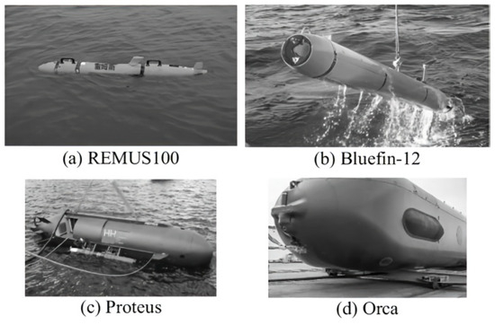
Figure 14.
US-based advanced UUV (reprinted with permission from [245]).
6.2. Advanced Navigation-Based UUV in European Countries
An anti-mine UUV known as the “Talisman” [246] that was able to carry four temporary mine suppressors was successfully constructed in the UK in 2008 [246]. All anti-mine tasks, including mine detection, verification, and suppression, were successfully completed by this aircraft. Another tiny UUV is the reusable mine suppressor “Archerfish” [246], which has a 104 mm diameter and an 880 mm length. Depending on the type of operation, the “talisman” UUV may be adjusted with varying loads and has an open structural design. The “MASTT” [246] ultra-large UUV, developed in the UK in 2014, has a 2.75-m diameter and an 8.85 m long titanium alloy hull.
The UUV can carry a variety of equipment, including miniature frogmen, and has a range of more than 2500 nautical miles [246]. Furthermore, several European nations—Norway’s “Hugin 1000” [247] series, France’s “Alister” [247] series, Sweden’s ”AUV62-MR”, and “MuMNS” [247] series—have also produced UUVs that are appropriate for their real needs [247]. Figure 15 displays the sophisticated UUVs from European nations. European nations started to focus on the establishment of large, ultra-large UUVs in response to the UUV’s limited capabilities, small platform, and other drawbacks [247]. They also took into account the requirements of upcoming missions and the marine environment, which included navigation, image resolution, and other higher requirements [247].
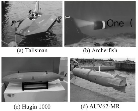
Figure 15.
Advanced UUV in European countries (reprinted with permission from [245]).
European nations started developing large, ultra-large UUVs in response to the UUV’s limited capabilities [247], small platform, and other drawbacks, examining and exploring the oceans while taking safety and dependability into account [6]. According to existing developments, themes, organizers, goals, and kinds, European nations are now the most concerned about autonomous underwater vehicle development [248,249]. They also started to take into account the demands of upcoming missions and the marine environment, which will increase the need for navigation, image resolution, and other capabilities [247].
6.3. Advanced Navigation-Based UUV in Russia
Due to the fall of the Soviet Union, Russia has given the study and creation of UUV applications top priority [247,250]. Russia has created a number of large-scale UUVs since the turn of the twenty-first century in order to meet its own maritime requirements [247,251]. The “harpsichord-2” [251] passed testing in 2018. This particular model of UUV had a 300 km range, could descend to a depth of 6000 m, and was outfitted with an autonomous navigational device that allowed it to stay in contact with the mother ship. It has previously conducted subsurface search and rescue operations in Arctic seas and was mostly utilized for ocean exploration [252]. The design idea for a “Surrogate” [251] UUV, which mimicked the physical field of several underwater vehicle types, was suggested by the Russian Design Bureau of “Ruby” [251] in 2016.
The nuclear-powered UUV “Poseidon” [251] was sent out for testing in 2019. This kind of UUV may travel up to 10,000 km at a velocity of over 100 knots while carrying a variety of payloads [251], including nuclear bombs, thanks to a miniature nuclear power component. It also performs exceptionally well in terms of acoustic stealth. Figure 16 depicts the sophisticated UUVs made in Russia. Following the breakup of the Soviet Union, Russia’s UUV development saw a prolonged period of slow development, mostly due to political and economic factors [251]. Nevertheless, there has been a notable increase in the number of UUVs under development and actively used in service, coinciding with the unmanned platforms’ progressive ascent within Russia’s fleet.
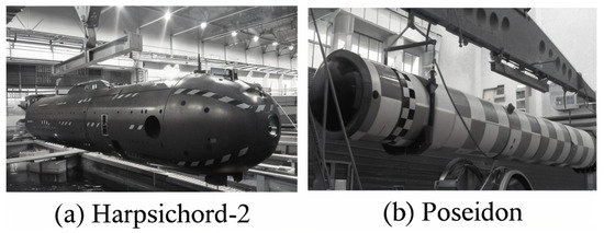
Figure 16.
Advanced UUV in Russia (reprinted with permission from [245]).
Concurrently, Russia’s UUVs have carved out a unique path marked by the prominence of big and ultra-large UUV platforms with nuclear propulsion systems, supplemented by smaller UUVs [247,251]. For this reason, it might be said that Russia is likewise working on building underwater vehicles to compete with other nations [251,253].
Due mainly to political and economic factors, Russia’s development of UUVs had a lengthy period of slow development after the fall of the Soviet Union. However, in tandem with the increasing prominence of unmanned vehicles in Russia’s arsenal, there has also been a notable increase in the number of UUVs under development and actively deployed in operation. Simultaneously, Russia’s UUVs have outlined a unique path marked by the prominence of big and super-large UUV systems equipped with nuclear propulsion systems, supplemented by smaller UUVs.
7. Future Prospects of Navigation Systems and Sensors of UUV
7.1. Sonars’ Suitability for Geophysical Navigation
While multibeam sonars focus on a smaller region, they are nevertheless able to provide an accurate [15], three-dimensional picture of that area. Side-scan sonars capture an image of a large portion of the sea bottom. The majority of commercial UUVs have access to both; however [15,254], it is unclear which is better to be used by the navigational system. Geophysical data can be extracted more easily via a multibeam sonar than from a side-scan sonar, even though side-scan sonar devices have a considerably longer range and may be able to identify more objects [15]. Designing a UUV will need careful consideration of the respective navigational capabilities of various sonars in various settings [15].
7.2. Underwater Map Resolution Requirements
The issue of long-range, precise UUV navigation has been shown to have a practical answer in the form of a geophysically related navigation system [120]. On the other hand, it has been demonstrated that the accuracy and variance of such a map significantly affect the system’s performance [120]. The level of detail in the available charts will determine how feasible it is to use them for UUV operations over wide mission regions, utilizing current surveys and charts. Although a simulation with high-resolution mapping in a region with significant variation has produced good results [120], the performance change with image resolution and variance has not been shown. It is quite desired to have a system that can offer resolution and variety together with a gentle decline in performance.
7.3. Identifying and Categorizing Naturally Existing Underwater Features
The easiest characteristics to identify visually from side-scan sonar studies of bathymetric maps are the ridges and channels running parallel to the sea bottom [255,256]. A striking deficiency exists in many underwater habitats in distinct characteristics that are not sufficiently harmonious to be classified as point features [256]. The challenge of extracting features from sonar has been studied for interior, structured environments where acoustic returns are classed as line features [255,256]. However, bathymetric charts typically lack a relevant density of these features, save in the case of ports and harbors [256]. This suggests that in these kinds of situations, a UUV navigational system has to be able to gather and classify such elements [256].
Underwater sonar returns are unstructured and changeable [257], which calls for the examination of image processing methods such as neural networks, which have been used for the classification of noisy, partly viewable characteristics [257]. Establishing a workable method for obtaining geophysical properties from sonar data that is compatible with current bathymetric surveys is crucial [257]. Nevertheless, the application of these categorization methods to underwater sonar data is not well documented [257].
7.4. Using Contour Alignment in Navigation
A technique of geophysical UUV navigation is suggested by the extraction and matching of contours [258], as many bathymetric charts include data about depth in contour form. A contouring system may have an advantage over a grid-based system in that less precision is needed from the sonar detectors and the onboard map [258]. However, the idea of the Internet of Underwater Things (IoUT) is making a significant impact in a number of places, including average-sized harbors and modest research sites, along with vast uncharted oceanic regions in today’s life [259].
Based on that, a global cost factor is minimized in order to align the extracted outlines [260,261]. Despite being a single-pass approach, this one is limited to huge datasets and computationally costly. In a more appropriate contour extraction technique, a set of B-spline parameters and curve primitives is provided to follow distorted and obscured contours [262]. However, its application to chaotic sonar data indicates that significant pre-processing is required to obtain the paper’s stated performance. In, an alternate approach specifically intended for underwater navigation is put forward [262]. It makes use of bathymetric chart-derived key spots to facilitate navigation. Partial differential equations and an EKF are used to find scale-invariant critical points [262].
The computing needs for this method’s stability need to be further investigated for low-cost vehicles as well (Figure 17). The autonomous section will undergo a revolution if sensors are developed further, become more affordable, and may be used for oceanographic study and exploration. In recent days, scientists have also been working to enhance the qualities of their sensors.
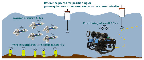
Figure 17.
New technologies for low-cost autonomous underwater vehicles (reprinted with permission from [263]).
A more modern method to improve the autonomous vehicles may be found in the upcoming days [263]. This explains how to use wavelet methods to match noisy data to contours created from 3D bathymetric data [264]. The wavelet methodology is theoretically less susceptible to distortion than gradient methods, and the results are comprehensive. If this technology is appropriate for underwater navigation, it might be studied through simulations with mission data [262,263].
8. Conclusions
A brief analysis of the sensor methodologies and approaches in today’s world in use for underwater mapping has been provided, along with an overview of their appropriateness for the various tasks that UUVs must carry out [265]. UUV navigation, along with sensor present problems, has been noted, and several recommendations for future studies have been made in light of these problems. It has been determined that although inertial and acoustic navigation systems are better developed than geophysical approaches, their performance is essentially constrained by their expense, assortment, and freely circulated correction cycle over long missions.
The growing endurance of UUV systems can be attributed to advancements in energy storage and propulsion technologies as well [266,267]. The navigation system’s precision is now the limiting constraint for UUV operation [234]. Because of this, UUVs are unable to complete lengthy survey missions that call for precise placement. The price and range of UUVs are limited by the employment of costly inertial and acoustic systems as well as sensors, even though they can help lessen the loss of navigational accuracy throughout a UUV mission [268].
By employing current images of a UUV target region, geophysical approaches could provide navigation that may be more accurate and less expensive. Nevertheless, the utility of these techniques is limited by the need for a current map and the challenges associated with feature recognition [234]. Given the chaotic environment of the underwater environment and the lack of thorough investigation into the necessary methodologies for effective geophysical navigation, it is suggested that noise-resistant classifiers, such as neural networks, be used to process incomplete data [269]. These findings are easily applicable to other unstructured situations when GPS isn’t accessible for navigation.
The current issue in UUV guidance is to minimize the time-varying drift of present navigation systems during extended missions by employing techniques that don’t need a significant detour from the mission nor come with a high deployment cost. These issues can be resolved by significantly extending the range of the current acoustic beacon systems; however, this is unlikely given the energy constraints and accuracy issues associated with long-range acoustic transmissions [270]. As a result, long-range underwater navigation requires the UUV to use its immediate surroundings, and its accuracy will inevitably be limited by how suitable the surroundings are for navigation.
In many areas of marine robotics, machine learning is essential and dominates how AI is now seen, although it is now in the planning and building stages. Although the development of autonomous underwater systems is already concentrating on AI principles and techniques, widespread deployment to commercial systems is currently in its early stages [271]. However, significant progress has been made in recent years, particularly in combining several capabilities (perception, navigation, and sophisticated control) into a single system and with the first methods of interaction and self-managing.
Major areas that could benefit from the development of AI are logistics, coordination of multi-robot deployment, spatiotemporal scheduling, mission planning, mission breakdown, task completion [272], action tracking [273], behavior composition using behavior trees, docking and homing [274], underwater obstacle avoidance [275,276], machine learning of system disturbances (e.g., ML-based magnetic field distortion compensation) [277], guidance and navigation, including SLAM and similar probabilistic sensor-fusion approaches [278], environment perception and representation [279], and object detection and classification [280]. The issues of autonomous extraction of features and recognition from pressure sensors, DVL sensors, and acoustic-like sonar detectors that provide the greatest degree of precision and range in the submerged setting must be addressed by future navigational techniques along with proper algorithms to compensate for drifts as much as possible.
Author Contributions
Conceptualization, K.P., M.M.S.; investigation, M.M.S., M.K., N.P.; data curation, M.M.S., M.K.; writing—original draft preparation, M.M.S.; writing—review and editing, M.M.S.; supervision, K.P. All authors have read and agreed to the published version of the manuscript.
Funding
This work is supported by UMass Dartmouth’s Marine and Undersea Technology (MUST) Research Program funded by the Office of Naval Research (ONR) under Grants No. N00014-23-1-2141.
Institutional Review Board Statement
Not applicable.
Informed Consent Statement
Not applicable.
Data Availability Statement
No new data were created or analyzed in this study. Data sharing is not applicable to this review.
Conflicts of Interest
The authors declare no conflicts of interest.
Abbreviations
The following abbreviations are used in this manuscript:
| ADCP | Acoustic Doppler Current Profilers |
| AHRS | Altitude Heading Reference Systems |
| ASKF | Augmented State Kalman Filter |
| AUV | Autonomous Underwater Vehicle |
| BL | Bottom Lock |
| CTS | Constant Time SLAM |
| CML | Concurrent Mapping and Localization |
| DOE | Diffractive Optical Element |
| DVL | Doppler Velocity Logger |
| DVS | Doppler Velocity Sensor |
| DR | Dead Rocking |
| EKF | Extended Kalman Filter |
| EMC | Electromagnetic Compatibility |
| FPGA | Field Programmable Gate Array |
| GNSS | Global Navigation Satellite System |
| GRUs | Gated Recurrent Units |
| IMU | Inertial Measurement Unit |
| INS | Inertial Navigation System |
| IoUT | Internet of Underwater Things |
| KF | Kalman Filter |
| LBL | Long Baseline |
| MAK | Mapping Augmented Kalman |
| MBESs | Multibeam Echo Sounders |
| MCP | Maritime Connectivity Platform |
| MEMS | Micro-electro Mechanical Systems |
| NS | Navigating System |
| ONR | Office of Naval Research |
| PEMFC | Proton Exchange Membrane Fuel Cell |
| ROV | Remotely Operated Vehicle |
| SBPs | Subbottom Profilers |
| SIS | Sequential Importance Sampling |
| SLAM | Simultaneous Localization And Mapping |
| SSSs | Sidescan Sonars |
| TAN | Terrain-aided Navigation |
| UKF | Unscented Kalman Filter |
| USBL | Ultrashort Baseline |
| UUV | Unmanned Underwater Vehicle |
| v-SLAM | Visual Simultaneous Localization And Mapping |
| WL | Water Lock |
References
- Huang, H.M. Autonomy levels for unmanned systems (ALFUS) framework: Safety and application issues. In Proceedings of the 2007 Workshop on Performance Metrics for Intelligent Systems, Washington, DC, USA, 28–30 August 2007; pp. 48–53. [Google Scholar]
- Balestrieri, E.; Daponte, P.; De Vito, L.; Lamonaca, F. Sensors and Measurements for Unmanned Systems: An Overview. Sensors 2021, 21, 1518. [Google Scholar] [CrossRef] [PubMed]
- Wang, X. Active fault tolerant control for unmanned underwater vehicle with sensor faults. IEEE Trans. Instrum. Meas. 2020, 69, 9485–9495. [Google Scholar] [CrossRef]
- Lin, C.; Wang, H.; Fu, M.; Yuan, J.; Gu, J. A gated recurrent unit-based particle filter for unmanned underwater vehicle state estimation. IEEE Trans. Instrum. Meas. 2020, 70, 1000612. [Google Scholar] [CrossRef]
- Martin, B.; Tarraf, D.C.; Whitmore, T.C.; DeWeese, J.; Kenney, C.; Schmid, J.; DeLuca, P. Advancing Autonomous Systems; Rand Corporation: Santa Monica, CA, USA, 2019; pp. 9–11. [Google Scholar]
- Sánchez, P.J.B.; Papaelias, M.; Márquez, F.P.G. Autonomous underwater vehicles: Instrumentation and measurements. IEEE Instrum. Meas. Mag. 2020, 23, 105–114. [Google Scholar] [CrossRef]
- Petillot, Y.R.; Antonelli, G.; Casalino, G.; Ferreira, F. Underwater robots: From remotely operated vehicles to intervention-autonomous underwater vehicles. IEEE Robot. Autom. Mag. 2019, 26, 94–101. [Google Scholar] [CrossRef]
- Paull, L.; Saeedi, S.; Seto, M.; Li, H. AUV Navigation and Localization: A Review. IEEE J. Ocean. Eng. 2014, 39, 131–149. [Google Scholar] [CrossRef]
- Hagen, P.E.; Midtgaard, O.; Hasvold, O. Making AUVs Truly Autonomous. In Proceedings of the OCEANS 2007, Vancouver, BC, Canada, 29 September–4 October 2007; pp. 1–4. [Google Scholar] [CrossRef]
- Du, X.; Hu, X.; Hu, J.; Sun, Z. An adaptive interactive multi-model navigation method based on UUV. Ocean Eng. 2023, 267, 113217. [Google Scholar] [CrossRef]
- Subad, R.A.S.I.; Cross, L.B.; Park, K. Soft robotic hands and tactile sensors for underwater robotics. Appl. Mech. 2021, 2, 356–382. [Google Scholar] [CrossRef]
- Qin, J.; Li, M.; Li, D.; Zhong, J.; Yang, K. A survey on visual navigation and positioning for autonomous UUVs. Remote Sens. 2022, 14, 3794. [Google Scholar] [CrossRef]
- Melo, J.; Matos, A. Survey on advances on terrain based navigation for autonomous underwater vehicles. Ocean Eng. 2017, 139, 250–264. [Google Scholar] [CrossRef]
- McNelly, B.P.; Whitcomb, L.L.; Brusseau, J.P.; Carr, S.S. Evaluating Integration of Autonomous Underwater Vehicles into Port Protection. In Proceedings of the OCEANS 2022, Hampton Roads, VA, USA, 17–20 October 2022; pp. 1–8. [Google Scholar] [CrossRef]
- Stutters, L.; Liu, H.; Tiltman, C.; Brown, D.J. Navigation Technologies for Autonomous Underwater Vehicles. IEEE Trans. Syst. Man Cybern. Part C (Appl. Rev.) 2008, 38, 581–589. [Google Scholar] [CrossRef]
- Bjerkeng, M.; Kirkhus, T.; Caharija, W.; T. Thielemann, J.; B. Amundsen, H.; Johan Ohrem, S.; Ingar Grøtli, E. ROV navigation in a fish cage with laser-camera triangulation. J. Mar. Sci. Eng. 2021, 9, 79. [Google Scholar] [CrossRef]
- González-García, J.; Gómez-Espinosa, A.; Cuan-Urquizo, E.; García-Valdovinos, L.G.; Salgado-Jiménez, T.; Escobedo Cabello, J.A. Autonomous underwater vehicles: Localization, navigation, and communication for collaborative missions. Appl. Sci. 2020, 10, 1256. [Google Scholar] [CrossRef]
- Grenon, G.; An, P.; Smith, S.; Healey, A. Enhancement of the inertial navigation system for the Morpheus autonomous underwater vehicles. IEEE J. Ocean. Eng. 2001, 26, 548–560. [Google Scholar] [CrossRef]
- Hegrenæs, Ø.; Ramstad, A.; Pedersen, T.; Velasco, D. Validation of a new generation DVL for underwater vehicle navigation. In Proceedings of the 2016 IEEE/OES Autonomous Underwater Vehicles (AUV), Tokyo, Japan, 6–9 November 2016; pp. 342–348. [Google Scholar] [CrossRef]
- Medagoda, L.; Kinsey, J.C.; Eilders, M. Autonomous Underwater Vehicle localization in a spatiotemporally varying water current field. In Proceedings of the 2015 IEEE International Conference on Robotics and Automation (ICRA), Seattle, WA, USA, 26–30 May 2015; pp. 565–572. [Google Scholar] [CrossRef]
- Stanway, M.J. Water profile navigation with an Acoustic Doppler Current Profiler. In Proceedings of the OCEANS’10 IEEE SYDNEY, Sydney, Australia, 24–27 May 2010; pp. 1–5. [Google Scholar] [CrossRef]
- Chemori, A.; Kuusmik, K.; Salumäe, T.; Kruusmaa, M. Depth control of the biomimetic U-CAT turtle-like AUV with experiments in real operating conditions. In Proceedings of the 2016 IEEE International Conference on Robotics and Automation (ICRA), Stockholm, Sweden, 16–21 May 2016; pp. 4750–4755. [Google Scholar] [CrossRef]
- Hanson, C.E.; Woo, L.M.; Thomson, P.G.; Pattiaratchi, C.B. Observing the ocean with gliders: Techniques for data visualization and analysis. Oceanography 2017, 30, 222–227. [Google Scholar] [CrossRef][Green Version]
- Allotta, B.; Costanzi, R.; Ridolfi, A.; Colombo, C.; Bellavia, F.; Fanfani, M.; Pazzaglia, F.; Salvetti, O.; Moroni, D.; Pascali, M.A.; et al. The ARROWS project: Adapting and developing robotics technologies for underwater archaeology. IFAC-PapersOnLine 2015, 48, 194–199. [Google Scholar] [CrossRef]
- Liu, H.; Wang, Z.; Shan, R.; He, K.; Zhao, S. Research into the integrated navigation of a deep-sea towed vehicle with USBL/DVL and pressure gauge. Appl. Acoust. 2020, 159, 107052. [Google Scholar] [CrossRef]
- Pararas. Turtle: A Revolutionary Submarine. Available online: https://www.drgeorgepc.com/Turtle.html (accessed on 19 January 2025).
- Allard, Y.; Shahbazian, E.; Isenor, A. Unmanned Underwater Vehicle (UUV) Information Study; Defence Research and Development Canada: Ottawa, ON, Canada, 2014.
- Ignatious, H.A.; Hesham-El-Sayed; Khan, M. An overview of sensors in Autonomous Vehicles. Procedia Comput. Sci. 2022, 198, 736–741. [Google Scholar] [CrossRef]
- Blidberg, D.R. The development of autonomous underwater vehicles (AUV); a brief summary. In Proceedings of the IEEE ICRA, Seoul, Republic of Korea, 21–26 May 2001; Volume 4, pp. 122–129. [Google Scholar]
- Beard, R.; Lawton, J.; Hadaegh, F. A coordination architecture for spacecraft formation control. IEEE Trans. Control Syst. Technol. 2001, 9, 777–790. [Google Scholar] [CrossRef]
- Yoerger, D.R.; Bradley, A.M.; Jakuba, M.; German, C.R.; Shank, T.; Tivey, M. Autonomous and remotely operated vehicle technology for hydrothermal vent discovery, exploration, and sampling. Oceanography 2007, 20, 152–161. [Google Scholar] [CrossRef]
- Yoerger, D.R.; Jakuba, M.; Bradley, A.M.; Bingham, B. Techniques for deep sea near bottom survey using an autonomous underwater vehicle. In Robotics Research: Results of the 12th International Symposium ISRR; Springer: Berlin/Heidelberg, Germany, 2007; pp. 416–429. [Google Scholar]
- Jakuba, M.V.; Roman, C.N.; Singh, H.; Murphy, C.; Kunz, C.; Willis, C.; Sato, T.; Sohn, R.A. Long-baseline acoustic navigation for under-ice autonomous underwater vehicle operations. J. Field Robot. 2008, 25, 861–879. [Google Scholar] [CrossRef]
- McPhail, S. Autosub6000: A deep diving long-range AUV. J. Bionic Eng. 2009, 6, 55–62. [Google Scholar] [CrossRef]
- Wynn, R.B.; Huvenne, V.A.; Le Bas, T.P.; Murton, B.J.; Connelly, D.P.; Bett, B.J.; Ruhl, H.A.; Morris, K.J.; Peakall, J.; Parsons, D.R.; et al. Autonomous Underwater Vehicles (AUVs): Their past, present and future contributions to the advancement of marine geoscience. Mar. Geol. 2014, 352, 451–468. [Google Scholar] [CrossRef]
- Wang, C.; Cheng, C.; Cao, C.; Guo, X.; Pan, G.; Zhang, F. An Invariant Filtering Method Based on Frame Transformed for Underwater INS/DVL/PS Navigation. J. Mar. Sci. Eng. 2024, 12, 1178. [Google Scholar] [CrossRef]
- Murton, B.J.; Rouse, I.P.; Millard, N.W.; Flewellen, C.G. Multisensor, deep-towed instrument explores ocean floor. Eos Trans. Am. Geophys. Union 1992, 73, 225–228. [Google Scholar] [CrossRef]
- Scheirer, D.S.; Fornari, D.J.; Humphris, S.E.; Lerner, S. High-resolution seafloor mapping using the DSL-120 sonar system: Quantitative assessment of sidescan and phase-bathymetry data from the Lucky Strike segment of the Mid-Atlantic Ridge. Mar. Geophys. Res. 2000, 21, 121–142. [Google Scholar] [CrossRef]
- Jones, J.; Chao, Y. Utilizing Ocean Thermal Energy in a Submarine Robot; Technical Report, NASA Tech Briefs; NASA: Washington, DC, USA, 2009.
- National Research Council. Review of ONR’s Uninhabited Combat Air Vehicles Program; National Academies Press: Washington, DC, USA, 2000.
- Zhang, B.; Xu, W.; Lu, C.; Lu, Y.; Wang, X. Review of low-loss wireless power transfer methods for autonomous underwater vehicles. IET Power Electron. 2022, 15, 775–788. [Google Scholar] [CrossRef]
- Kamp, J.; Curtin, T.B.; Dryden, J.; Button, R.W. A Survey of Missions for Unmanned Undersea Vehicles; Coherent Digital: Alexandria, VA, USA, 2009. [Google Scholar]
- Jones, J.A. A New Technique for Robot Vision in Autonomous Underwater Vehicles Using the Color Shift in Underwater Imaging. Ph.D. Thesis, Naval Postgraduate School, Monterey, CA, USA, 2017. [Google Scholar]
- Roberts, H.; Shedd, W.; Hunt, J., Jr. Dive site geology: DSV ALVIN (2006) and ROV JASON II (2007) dives to the middle-lower continental slope, northern Gulf of Mexico. Deep Sea Res. Part II Top. Stud. Oceanogr. 2010, 57, 1837–1858. [Google Scholar] [CrossRef]
- Matouš, J.; Paliotta, C.; Pettersen, K.Y.; Varagnolo, D. The Hand Position Concept for Control of Underactuated Underwater Vehicles. IEEE Trans. Control Syst. Technol. 2024, 32, 2223–2239. [Google Scholar] [CrossRef]
- Panda, J.P.; Mitra, A.; Warrior, H.V. A review on the hydrodynamic characteristics of autonomous underwater vehicles. Proc. Inst. Mech. Eng. Part M J. Eng. Marit. Environ. 2021, 235, 15–29. [Google Scholar] [CrossRef]
- Sahoo, A.; Dwivedy, S.K.; Robi, P. Advancements in the field of autonomous underwater vehicle. Ocean Eng. 2019, 181, 145–160. [Google Scholar] [CrossRef]
- Kwon, L.; Kang, J.G.; Baik, K.D.; Kim, K.; Ahn, C. Advancement and applications of PEMFC energy systems for large-class unmanned underwater vehicles: A review. Int. J. Hydrogen Energy 2024, 79, 277–294. [Google Scholar] [CrossRef]
- Singh, R.K.; Sangeetha, R. Review of EMC standards for underwater vehicles. Results Eng. 2024, 24, 103068. [Google Scholar] [CrossRef]
- He, Y.; Zhang, H. Analysis of Characteristics on a Compressed Air Power System Generating Supercavitation Drag Reduction for Underwater Vehicles. Energies 2024, 17, 1735. [Google Scholar] [CrossRef]
- Akgun, I.; Dincer, I. Development of a smart powering system with ammonia fuel cells and internal combustion engine for submarines. Energy 2024, 294, 130747. [Google Scholar] [CrossRef]
- Budiyono, A. Advances in unmanned underwater vehicles technologies: Modeling, control and guidance perspectives. Indian J. Mar. Sci. 2009, 38, 282–295. [Google Scholar]
- Bandyopadhyay, P.R. Trends in biorobotic autonomous undersea vehicles. IEEE J. Ocean. Eng. 2005, 30, 109–139. [Google Scholar] [CrossRef]
- Yun, X.; Bachmann, E.R.; McGhee, R.B.; Whalen, R.H.; Roberts, R.L.; Knapp, R.G.; Healey, A.J.; Zyda, M.J. Testing and evaluation of an integrated GPS/INS system for small AUV navigation. IEEE J. Ocean. Eng. 1999, 24, 396–404. [Google Scholar] [CrossRef]
- An, P.; Healey, A.; Park, J.; Smith, S. Asynchronous data fusion for AUV navigation via heuristic fuzzy filtering techniques. In Proceedings of the Oceans ’97. MTS/IEEE Conference Proceedings, Halifax, NS, Canada, 6–9 October 1997; Volume 1, pp. 397–402. [Google Scholar] [CrossRef]
- Beis, A.; Marco, D.; Brutzman, D. A Finite Element Analysis of the Nps Autonomous Underwater Vehicle (AUV) Hull Intended to Operate in Deep Waters. Ph.D. Thesis, Naval Postgraduate School, Monterey, CA, USA, 2001. [Google Scholar]
- Podder, T.; Antonelli, G.; Sarkar, N. Fault tolerant control of an autonomous underwater vehicle under thruster redundancy: Simulations and experiments. In Proceedings of the Proceedings 2000 ICRA. Millennium Conference. IEEE International Conference on Robotics and Automation, Symposia Proceedings (Cat. No.00CH37065), San Francisco, CA, USA, 24–28 April 2000; Volume 2, pp. 1251–1256. [Google Scholar] [CrossRef]
- Healey, A.J.; Rock, S.M.; Cody, S.; Miles, D.; Brown, J.P. Toward an improved understanding of thruster dynamics for underwater vehicles. IEEE J. Ocean. Eng. 1995, 20, 354–361. [Google Scholar] [CrossRef]
- Riedel, J.S.; Healey, A.J.; Marco, D.B.; Beyazay, B. Design and development of low cost variable buoyancy system for the soft grounding of autonomous underwater vehicles. In Proceedings of the International Symposium on Unmanned Untethered Submersible Technology, Durham, NH, USA, 22–25 August 1999; pp. 427–438. [Google Scholar]
- Bicho, E.; Mallet, P.; Schöner, G. Target representation on an autonomous vehicle with low-level sensors. Int. J. Robot. Res. 2000, 19, 424–447. [Google Scholar] [CrossRef]
- Caccia, M.; Veruggio, G. Acoustic motion estimation and guidance for unmanned underwater vehicles. Int. J. Syst. Sci. 1999, 30, 929–938. [Google Scholar] [CrossRef]
- Riedel, J.S.; Healey, A.J. Estimation of directional wave spectra from an autonomous underwater vehicle (AUV). In Proceedings of the 11th International Symposium on Unmanned Untethered Submersible Technology (UUST’99), Durham, NH, USA, 22–25 August 1999; pp. 140–149. [Google Scholar]
- Jin, K.; Yan, X.; Li, J.; Zhou, M.; Fu, K.; Wei, X.; Meng, F.; Liu, J. Recent progress in aqueous underwater power batteries. Discov. Appl. Sci. 2024, 6, 441. [Google Scholar] [CrossRef]
- Lee, P.M.; Jun, B.H.; Kim, K.; Lee, J.; Aoki, T.; Hyakudome, T. Simulation of an inertial acoustic navigation system with range aiding for an autonomous underwater vehicle. IEEE J. Ocean. Eng. 2007, 32, 327–345. [Google Scholar] [CrossRef]
- Eustice, R.M.; Singh, H.; Whitcomb, L.L. Synchronous-clock, one-way-travel-time acoustic navigation for underwater vehicles. J. Field Robot. 2011, 28, 121–136. [Google Scholar] [CrossRef]
- Saksvik, I.B.; Alcocer, A.; Hassani, V. A deep learning approach to dead-reckoning navigation for autonomous underwater vehicles with limited sensor payloads. In Proceedings of the OCEANS 2021: San Diego–Porto, San Diego, CA, USA, 20–23 September 2021; pp. 1–9. [Google Scholar]
- Kepper, J.H.; Claus, B.C.; Kinsey, J.C. A navigation solution using a MEMS IMU, model-based dead-reckoning, and one-way-travel-time acoustic range measurements for autonomous underwater vehicles. IEEE J. Ocean. Eng. 2018, 44, 664–682. [Google Scholar] [CrossRef]
- Yoo, T.S. DVL/RPM based velocity filter aiding in the underwater vehicle integrated inertial navigation system. J. Sens. Technol. 2014, 4, 154–164. [Google Scholar] [CrossRef]
- Miller, A.; Miller, B.; Miller, G. Navigation of underwater drones and integration of acoustic sensing with onboard inertial navigation system. Drones 2021, 5, 83. [Google Scholar] [CrossRef]
- McEwen, R.; Thomas, H.; Weber, D.; Psota, F. Performance of an AUV navigation system at Arctic latitudes. IEEE J. Ocean. Eng. 2005, 30, 443–454. [Google Scholar] [CrossRef]
- Griffiths, G.; Millard, N.; McPhail, S.; Riggs, J. Effect of upgrades on the reliability of the Autosub AUV. In Proceedings of the 13th International Symposium on Unmanned Untethered Submersible Technology, Durham, NH USA, 24–27 August 2003. [Google Scholar]
- Grewal, M.S. Global Positioning Systems, Inertial Navigation, and Integration; John Wiley & Sons: Hoboken, NJ, USA, 2007. [Google Scholar]
- Kalman, R.E. A new approach to linear filtering and prediction problems. J. Basic Eng. 1960, 82, 35–45. [Google Scholar] [CrossRef]
- Welch, G.; Bishop, G. An Introduction to the Kalman Filter; University of North Carolina at Chapel Hill: Chapel Hill, NC, USA, 1995. [Google Scholar]
- Song, T.J. Experimental Evaluation of Underwater Semantic SLAM. Ph.D. Thesis, Massachusetts Institute of Technology, Cambridge, MA, USA, 2024. [Google Scholar]
- Healey, A.J.; An, E.; Marco, D. Online compensation of heading sensor bias for low-cost AUVs. In Proceedings of the 1998 Workshop on Autonomous Underwater Vehicles (Cat. No. 98CH36290), Cambridge, MA, USA, 21 August 1998; pp. 35–42. [Google Scholar]
- Bliksted, L.M. High-Performance Doppler-Inertial Navigation-Experimental Result. In Proceedings of the Conference Proceedings of OCEANS 2000 MTS/IEEE, Providence, RI, USA, 11–14 September 2000; Volume 2, pp. 1449–1456. [Google Scholar]
- Julier, S.J.; Uhlmann, J.K.; Durrant-Whyte, H.F. A new approach for filtering nonlinear systems. In Proceedings of the 1995 American Control Conference-ACC’95, Seattle, WA, USA, 21–23 June 1995; Volume 3, pp. 1628–1632. [Google Scholar]
- Julier, S.J.; Uhlmann, J.K. New extension of the Kalman filter to nonlinear systems. In Proceedings of the Signal Processing, Sensor Fusion, and Target Recognition VI; SPIE: Bellingham, WA, USA, 1997; Volume 3068, pp. 182–193. [Google Scholar]
- Jalal, F.; Nasir, F. Underwater navigation, localization and path planning for autonomous vehicles: A review. In Proceedings of the 2021 International Bhurban Conference on Applied Sciences and Technologies (IBCAST), Islamabad, Pakistan, 12–16 January 2021; pp. 817–828. [Google Scholar]
- Wan, E.A.; Van Der Merwe, R. The unscented Kalman filter for nonlinear estimation. In Proceedings of the IEEE 2000 Adaptive Systems for Signal Processing, Communications, and Control Symposium (Cat. No. 00EX373), Lake Louise, AB, Canada, 4 October 2000; pp. 153–158. [Google Scholar]
- Ristic, B.; Arulampalam, S.; Gordon, N. Beyond the Kalman Filter: Particle Filters for Tracking Applications; Artech House: Norwood, MA, USA, 2003. [Google Scholar]
- Gustafsson, F.; Gunnarsson, F.; Bergman, N.; Forssell, U.; Jansson, J.; Karlsson, R.; Nordlund, P.J. Particle filters for positioning, navigation, and tracking. IEEE Trans. Signal Process. 2002, 50, 425–437. [Google Scholar] [CrossRef]
- Zhang, J.; Xu, B.; Wang, Z.; Razzaqi, A.A.; Wang, C.; Liu, X. An Implicit Acoustic Navigation Sensor-Based Method for AUV Cluster Cooperative Navigation and Sensitivity Analysis of DSUA Sensor. IEEE Sens. J. 2024, 24, 32343–32355. [Google Scholar] [CrossRef]
- Menna, B.V.; Villar, S.A.; Acosta, G.G. Particle Filter based Autonomous Underwater Vehicle Navigation System aided thru acoustic communication ranging. In Proceedings of the Global Oceans 2020: Singapore—U.S. Gulf Coast, Biloxi, MS, USA, 5–30 October 2020; pp. 1–10. [Google Scholar] [CrossRef]
- Cheeseman, P.; Smith, R.; Self, M. A stochastic map for uncertain spatial relationships. In Proceedings of the 4th International Symposium on Robotic Research; MIT Press Cambridge: Cambridge, MA, USA, 1987; pp. 467–474. [Google Scholar]
- Csorba, M. Simultaneous Localisation and Map Building. Ph.D. Thesis, University of Oxford, Oxford, UK, 1997. [Google Scholar]
- Newman, P.; Ho, K. SLAM-loop closing with visually salient features. In Proceedings of the 2005 IEEE International Conference on Robotics and Automation, Barcelona, Spain, 18–22 April 2005; pp. 635–642. [Google Scholar]
- Dissanayake, M.G.; Newman, P.; Clark, S.; Durrant-Whyte, H.F.; Csorba, M. A solution to the simultaneous localization and map building (SLAM) problem. IEEE Trans. Robot. Autom. 2001, 17, 229–241. [Google Scholar] [CrossRef]
- Thrun, S. Bayesian landmark learning for mobile robot localization. Mach. Learn. 1998, 33, 41–76. [Google Scholar] [CrossRef]
- Tena Ruiz, I.J. Enhanced Concurrent Mapping and Localisation Using Forward-Looking Sonar. Ph.D. Thesis, Heriot-Watt University, Edinburgh, UK, 2001. [Google Scholar]
- Ruiz, I.T.; Reed, S.; Petillot, Y.; Bell, J.; Lane, D.M. Concurrent mapping & localisation using side-scan sonar for autonomous navigation. In Proceedings of the International Symposium on Unmanned Untethered Submersible Technology, Durham, NH, USA, 24–27 August 2003. [Google Scholar]
- Fenwick, J.W.; Newman, P.M.; Leonard, J.J. Cooperative concurrent mapping and localization. In Proceedings of the Proceedings 2002 IEEE International Conference on Robotics and Automation (Cat. No. 02CH37292), Washington, DC, USA, 11–15 May 2002; Volume 2, pp. 1810–1817. [Google Scholar]
- Tardós, J.D.; Neira, J.; Newman, P.M.; Leonard, J.J. Robust mapping and localization in indoor environments using sonar data. Int. J. Robot. Res. 2002, 21, 311–330. [Google Scholar] [CrossRef]
- Montemerlo, M. FastSLAM: A Factored Solution to the Simultaneous Localization and Mapping Problem. In Proceedings of the AAAI02, Edmonton, AB, Canada, 28 July–1 August 2002. [Google Scholar]
- Leonard, J.; Newman, P. Consistent, convergent, and constant-time SLAM. In Proceedings of the IJCAI, Acapulco, Mexico, 9–15 August 2003; pp. 1143–1150. [Google Scholar]
- Williams, S.; Dissanayake, G.; Durrant-Whyte, H. Towards terrain-aided navigation for underwater robotics. Adv. Robot. 2001, 15, 533–549. [Google Scholar] [CrossRef]
- Olson, E.; Leonard, J.J.; Teller, S. Robust range-only beacon localization. IEEE J. Ocean. Eng. 2006, 31, 949–958. [Google Scholar] [CrossRef]
- Newman, P.M.; Leonard, J.J.; Rikoski, R.J. Towards constant-time SLAM on an autonomous underwater vehicle using synthetic aperture sonar. In Robotics Research. The Eleventh International Symposium: With 303 Figures; Springer: Berlin/Heidelberg, Germany, 2005; pp. 409–420. [Google Scholar]
- Edwards, J.R.; Schmidt, H.; LePage, K.D. Bistatic synthetic aperture target detection and imaging with an AUV. IEEE J. Ocean. Eng. 2001, 26, 690–699. [Google Scholar] [CrossRef]
- Thrun, S.; Liu, Y.; Koller, D.; Ng, A.Y.; Ghahramani, Z.; Durrant-Whyte, H. Simultaneous localization and mapping with sparse extended information filters. Int. J. Robot. Res. 2004, 23, 693–716. [Google Scholar] [CrossRef]
- Eustice, R.M. Large-Area Visually Augmented Navigation for Autonomous Underwater Vehicles. Ph.D. Thesis, Massachusetts Institute of Technology, Cambridge, MA, USA, 2005. [Google Scholar]
- Ruiz, I.T.; De Raucourt, S.; Petillot, Y.; Lane, D.M. Concurrent mapping and localization using sidescan sonar. IEEE J. Ocean. Eng. 2004, 29, 442–456. [Google Scholar] [CrossRef]
- Jung, J.; Park, J.; Choi, J.; Choi, H.T. Navigation of unmanned surface vehicles using underwater geophysical sensing. IEEE Access 2020, 8, 208707–208717. [Google Scholar] [CrossRef]
- Bosov, A.V.; Miller, G.B. Conditionally minimax nonlinear filter and Unscented Kalman filter: Empirical analysis and comparison. Autom. Remote Control 2019, 80, 1230–1251. [Google Scholar] [CrossRef]
- Mariani, S.; Ghisi, A. Unscented Kalman filtering for nonlinear structural dynamics. Nonlinear Dyn. 2007, 49, 131–150. [Google Scholar] [CrossRef]
- Sabet, M.T.; Sarhadi, P.; Zarini, M. Extended and Unscented Kalman filters for parameter estimation of an autonomous underwater vehicle. Ocean Eng. 2014, 91, 329–339. [Google Scholar] [CrossRef]
- Stanghellini, G.; Del Bianco, F.; Gasperini, L. OpenSWAP, an open architecture, low cost class of autonomous surface vehicles for geophysical surveys in the shallow water environment. Remote Sens. 2020, 12, 2575. [Google Scholar] [CrossRef]
- Tyren, C. Magnetic terrain navigation. In Proceedings of the 1987 5th International Symposium on Unmanned Untethered Submersible Technology, Durham, NH, USA, 22–24 June 1987; Volume 5, pp. 245–256. [Google Scholar]
- Tuoy, S.; Maekawa, T.; Patrikalalis, N. Interrogation of geophysical maps with uncertainty for AUV micro-navigation. In Proceedings of the OCEANS’93, Victoria, BC, Canada, 18–21 October 1993; pp. I181–I185. [Google Scholar]
- Zhang, F.; Chen, X.; Sun, M.; Yan, M.; Yang, D. Simulation study of underwater passive navigation system based on gravity gradient. In Proceedings of the IGARSS 2004. 2004 IEEE International Geoscience and Remote Sensing Symposium, Anchorage, AK, USA, 20–24 September 2004; Volume 5, pp. 3111–3113. [Google Scholar]
- Leonard, J.J.; Bahr, A. Autonomous underwater vehicle navigation. In Springer Handbook of Ocean Engineering; Springer: Cham, Switzerland, 2016; pp. 341–358. [Google Scholar]
- Howell, B.P. Evaluation of Neural Networks for Data Classification, Recognition, and Navigation in the Marine Environment. Ph.D. Thesis, Florida Institute of Technology, Melbourne, FL, USA, 2004. [Google Scholar]
- García, R.; Puig, J.; Ridao, P.; Cufi, X. Augmented state Kalman filtering for AUV navigation. In Proceedings of the Proceedings 2002 IEEE International Conference on Robotics and Automation (Cat. No. 02CH37292), Washington, DC, USA, 11–15 May 2002; Volume 4, pp. 4010–4015. [Google Scholar]
- Nygren, I. Terrain Navigation for Underwater Vehicles. Ph.D. Thesis, KTH, Stockholm, Sweden, 2005. [Google Scholar]
- Carlstrom, J.; Nygren, I. Terrain navigation of the Swedish AUV62F vehicle. In Proceedings of the International Symposium on Unmanned Untethered Submersible Technology (UUST), Durham, NH, USA, 21–24 August 2005. [Google Scholar]
- Nygren, I.; Jansson, M. Recursive Terrain Navigation with the Correlation method for High Position Accuracy. In Proceedings of the International Symposium on Unmanned Untethered Submersible Technology (UUST), Durham, NH, USA, 24–27 August 2003. [Google Scholar]
- Bergman, N.; Ljung, L.; Gustafsson, F. Terrain navigation using Bayesian statistics. IEEE Control Syst. Mag. 1999, 19, 33–40. [Google Scholar]
- Bachmann, A.; Williams, S.B. Terrain aided underwater navigation-a deeper insight into generic monte carlo localization. In Proceedings of the Australasian Conference on Robotics and Automation, Brisbane, Australia, 1–3 December 2003. [Google Scholar]
- Karlsson, R.; Gustafsson, F. Particle filter for underwater terrain navigation. In Proceedings of the IEEE Workshop on Statistical Signal Processing, St. Louis, MO, USA, 28 September–1 October 2003; pp. 526–529. [Google Scholar]
- Bergman, N. Bayesian Inference in Terrain Navigation; Citeseer: Princeton, NJ, USA, 1997. [Google Scholar]
- Doucet, A.; De Freitas, N.; Gordon, N.J. (Eds.) Sequential Monte Carlo Methods in Practice; Springer: New York, NY, USA, 2001; Volume 1. [Google Scholar]
- Verma, V.; Thrun, S.; Simmons, R. Variable resolution particle filter. In Proceedings of the IJCAI, Acapulco, Mexico, 9–15 August 2003; pp. 976–984. [Google Scholar]
- Arulampalam, M.S.; Maskell, S.; Gordon, N.; Clapp, T. A tutorial on particle filters for online nonlinear/non-Gaussian Bayesian tracking. IEEE Trans. Signal Process. 2002, 50, 174–188. [Google Scholar] [CrossRef]
- Barker, L.D.; Jakuba, M.V.; Bowen, A.D.; German, C.R.; Maksym, T.; Mayer, L.; Boetius, A.; Dutrieux, P.; Whitcomb, L.L. Scientific challenges and present capabilities in underwater robotic vehicle design and navigation for oceanographic exploration under-ice. Remote Sens. 2020, 12, 2588. [Google Scholar] [CrossRef]
- Bao, J.; Li, D.; Qiao, X.; Rauschenbach, T. Integrated navigation for autonomous underwater vehicles in aquaculture: A review. Inf. Process. Agric. 2020, 7, 139–151. [Google Scholar] [CrossRef]
- Weydahl, H.; Gilljam, M.; Lian, T.; Johannessen, T.C.; Holm, S.I.; Hasvold, J.Ø. Fuel cell systems for long-endurance autonomous underwater vehicles–challenges and benefits. Int. J. Hydrogen Energy 2020, 45, 5543–5553. [Google Scholar] [CrossRef]
- Su, X.; Ullah, I.; Liu, X.; Choi, D. A review of underwater localization techniques, algorithms, and challenges. J. Sensors 2020, 2020, 6403161. [Google Scholar] [CrossRef]
- Barrera, C.; Padron, I.; Luis, F.; Llinas, O. Trends and challenges in unmanned surface vehicles (Usv): From survey to shipping. TransNav Int. J. Mar. Navig. Saf. Sea Transp. 2021, 15, 135–142. [Google Scholar] [CrossRef]
- Köser, K.; Frese, U. Challenges in underwater visual navigation and SLAM. In AI Technology for Underwater Robots; Springer: Cham, Switzerland, 2020; pp. 125–135. [Google Scholar]
- Reed, S.; Petillot, Y.; Bell, J. Model-based approach to the detection and classification of mines in sidescan sonar. Appl. Opt. 2004, 43, 237–246. [Google Scholar] [CrossRef] [PubMed]
- Bell, J.M.; Lane, D.M.; Dura, E. Seafloor Classification Using Contour Maps Recovered from Sidescan Sonar. In Proceedings of the Computer Aided Detection and Computer Aided Classification Conference, Halifax, NS, Canada, 1 November 2001. [Google Scholar]
- Yan, Z.; Zhang, J.; Zeng, J.; Tang, J. Three-dimensional path planning for autonomous underwater vehicles based on a whale optimization algorithm. Ocean Eng. 2022, 250, 111070. [Google Scholar] [CrossRef]
- Zhang, B.; Ji, D.; Liu, S.; Zhu, X.; Xu, W. Autonomous underwater vehicle navigation: A review. Ocean Eng. 2023, 273, 113861. [Google Scholar] [CrossRef]
- Min, H.; Fang, Y.; Wu, X.; Lei, X.; Chen, S.; Teixeira, R.; Zhu, B.; Zhao, X.; Xu, Z. A fault diagnosis framework for autonomous vehicles with sensor self-diagnosis. Expert Syst. Appl. 2023, 224, 120002. [Google Scholar] [CrossRef]
- Zhang, S.; Zhao, S.; An, D.; Liu, J.; Wang, H.; Feng, Y.; Li, D.; Zhao, R. Visual SLAM for underwater vehicles: A survey. Comput. Sci. Rev. 2022, 46, 100510. [Google Scholar] [CrossRef]
- Wang, D.; Wang, B.; Huang, H.; Xu, B.; Zhang, H. A Novel SINS/DVL Integrated Navigation Method Based on Different Track Models for Complex Environment. IEEE Trans. Instrum. Meas. 2024, 73, 8501912. [Google Scholar] [CrossRef]
- Li, H.; Wang, G.; Li, X.; Lian, Y. A Review of Underwater SLAM Technologies. In Proceedings of the 2023 5th International Conference on Robotics, Intelligent Control and Artificial Intelligence (RICAI), Hangzhou, China, 1–3 December 2023; pp. 215–225. [Google Scholar]
- Cheng, M.; Guan, Q.; Ji, F.; Cheng, J.; Chen, Y. Dynamic-detection-based trajectory planning for autonomous underwater vehicle to collect data from underwater sensors. IEEE Internet Things J. 2022, 9, 13168–13178. [Google Scholar] [CrossRef]
- Li, H.; Wu, X.; Zhang, Z.; Tan, X.; Pan, Y.; Dai, C.; Luo, D.; Ahmed, A.; Xu, Y. An extended-range wave-powered autonomous underwater vehicle applied to underwater wireless sensor networks. iScience 2022, 25, 104738. [Google Scholar] [CrossRef]
- Yang, S.; Zhang, X.; Liu, D.; Bai, W.; Liu, F. Geomagnetic Guided Underwater Navigation with Gradient Multi-Attention Neural Networks. IEEE Sens. J. 2024, 24, 40003–40016. [Google Scholar] [CrossRef]
- Nađ, Đ.; Mandić, F.; Mišković, N. Using autonomous underwater vehicles for diver tracking and navigation aiding. J. Mar. Sci. Eng. 2020, 8, 413. [Google Scholar] [CrossRef]
- Sathish, K.; Venkata, R.C.; Anbazhagan, R.; Pau, G. Review of localization and clustering in USV and AUV for underwater wireless sensor networks. Telecom 2023, 4, 43–64. [Google Scholar] [CrossRef]
- Ishak, P.N.I.; Kadir, H.A. An Estimating Orientation Using IMU Module for Autonomous Underwater Vehicle (AUV). Evol. Electr. Electron. Eng. 2022, 3, 987–997. [Google Scholar]
- Liu, X.; Ju, Y.; Liu, X.; Miao, S.; Zhang, W. An IMU fault diagnosis and information reconstruction method based on analytical redundancy for autonomous underwater vehicle. IEEE Sensors J. 2022, 22, 12127–12138. [Google Scholar] [CrossRef]
- Chang, C.W.; Yan, J.L.; Chang, C.N.; Wen, K.A. IMU-based real-time four-type gait analysis and classification and circuit implementation. In Proceedings of the 2022 IEEE Sensors, Dallas, TX, USA, 30 October–2 November 2022; pp. 1–4. [Google Scholar]
- Snyder, J. Doppler Velocity Log (DVL) navigation for observation-class ROVs. In Proceedings of the OCEANS 2010 MTS/IEEE SEATTLE, Seattle, WA, USA, 20–23 September 2010; pp. 1–9. [Google Scholar] [CrossRef]
- Topini, E.; Fanelli, F.; Topini, A.; Pebody, M.; Ridolfi, A.; Phillips, A.B.; Allotta, B. An experimental comparison of Deep Learning strategies for AUV navigation in DVL-denied environments. Ocean Eng. 2023, 274, 114034. [Google Scholar] [CrossRef]
- Cohen, N.; Klein, I. BeamsNet: A data-driven approach enhancing Doppler velocity log measurements for autonomous underwater vehicle navigation. Eng. Appl. Artif. Intell. 2022, 114, 105216. [Google Scholar] [CrossRef]
- Pan, S.; Xu, X.; Yao, Y.; Zhang, L.; Xia, M. A Novel DVL Aided Inertial Navigation Strategy for Long-Endurance Robust Positioning of AUVs. IEEE Trans. Intell. Veh. 2024, 1–14. [Google Scholar] [CrossRef]
- Liu, J.; Yu, T.; Wu, C.; Zhou, C.; Lu, D.; Zeng, Q. A Low-Cost and High-Precision Underwater Integrated Navigation System. J. Mar. Sci. Eng. 2024, 12, 200. [Google Scholar] [CrossRef]
- Tal, A.; Klein, I.; Katz, R. Inertial navigation system/Doppler velocity log (INS/DVL) fusion with partial DVL measurements. Sensors 2017, 17, 415. [Google Scholar] [CrossRef]
- Liu, P.; Wang, B.; Deng, Z.; Fu, M. A correction method for DVL measurement errors by attitude dynamics. IEEE Sensors J. 2017, 17, 4628–4638. [Google Scholar] [CrossRef]
- Yao, Y.; Xu, X.; Hou, L.; Deng, K.; Xu, X. A simple and precise correction method for DVL measurements under the dynamic environment. IEEE Trans. Veh. Technol. 2020, 69, 10750–10758. [Google Scholar] [CrossRef]
- Liu, P.; Wang, B.; Deng, Z.; Fu, M. INS/DVL/PS tightly coupled underwater navigation method with limited DVL measurements. IEEE Sens. J. 2018, 18, 2994–3002. [Google Scholar] [CrossRef]
- Liu, P.; Zhao, S.; Qing, L.; Ma, Y.; Lu, B.; Hou, D. A calibration method for DVL measurement errors based on observability analysis. In Proceedings of the 2019 Chinese Control Conference (CCC), Guangzhou, China, 27–30 July 2019; pp. 3851–3856. [Google Scholar]
- Sabet, M.; Nourmohammadi, H. Water velocity sensor with the ability to estimate the sideslip angle based on Bernoulli’s law for use in autonomous underwater vehicles. Ocean Eng. 2022, 263, 112252. [Google Scholar] [CrossRef]
- Miller, A.; Miller, B. Underwater target tracking using bearing-only measurements. J. Commun. Technol. Electron. 2018, 63, 643–649. [Google Scholar] [CrossRef]
- Napolitano, F.; Cretollier, F.; Pelletier, H. GAPS, combined USBL+ INS+ GPS tracking system for fast deployable & high accuracy multiple target positioning. In Proceedings of the Europe Oceans 2005, Brest, France, 20–23 June 2005; Volume 2, pp. 1415–1420. [Google Scholar]
- Peyronnet, J.P.; Person, R.; Rybicki, F. Posidonia 6000: A new long range highly accurate ultra short base line positioning system. In Proceedings of the IEEE Oceanic Engineering Society. OCEANS’98. Conference Proceedings (Cat. No. 98CH36259), Nice, France, 28 September–1 October 1998; Volume 3, pp. 1721–1727. [Google Scholar]
- Darling. Applied Acoustics Easytrak USBL Systems. Available online: https://www.aaetechnologiesgroup.com/applied-acoustics/products/easytrak-usbl-systems/ (accessed on 11 March 2016).
- Bannasch, R. Evologics R-Series, “usbl”, EvoLogics. Available online: https://www.evologics.com/usbl (accessed on 22 October 2024).
- Wang, W.; Zhu, M.; Yang, B. Positioning combination method of USBL using four-element stereo array. Sensors 2021, 21, 7722. [Google Scholar] [CrossRef]
- Bresciani, M.; Zacchini, L.; Topini, A.; Ridolfi, A.; Costanzi, R. Automatic target recognition and geolocalisation of natural gas seeps using an autonomous underwater vehicle. Control Eng. Pract. 2024, 145, 105864. [Google Scholar] [CrossRef]
- Jaffré, F.M.; Austin, T.C.; Allen, B.G.; Stokey, R.; Von Alt, C.J. Ultra short baseline acoustic receiver/processor. In Proceedings of the Europe Oceans 2005, Brest, France, 20–23 June 2005; Volume 2, pp. 1382–1385. [Google Scholar]
- Sanz, P.J.; Ridao, P.; Oliver, G.; Melchiorri, C.; Casalino, G.; Silvestre, C.; Petillot, Y.; Turetta, A. TRIDENT: A framework for autonomous underwater intervention missions with dexterous manipulation capabilities. IFAC Proc. Vol. 2010, 43, 187–192. [Google Scholar] [CrossRef]
- Ma, J.; Yu, Y.; Zhang, Y.; Zhu, X. An USBL/DR Integrated Underwater Localization Algorithm Considering Variations of Measurement Noise Covariance. IEEE Access 2022, 10, 23873–23884. [Google Scholar] [CrossRef]
- Cho, H.; Jeong, S.K.; Ji, D.H.; Tran, N.H.; Vu, M.T.; Choi, H.S. Study on control system of integrated unmanned surface vehicle and underwater vehicle. Sensors 2020, 20, 2633. [Google Scholar] [CrossRef]
- Ercis, F. Design and Construction of Unmanned Underwater Vehicle. Ph.D. Thesis, Middle East Technical University, Ankara, Türkiye, 2013. [Google Scholar]
- Allotta, B.; Caiti, A.; Costanzi, R.; Fanelli, F.; Fenucci, D.; Meli, E.; Ridolfi, A. A new AUV navigation system exploiting unscented Kalman filter. Ocean Eng. 2016, 113, 121–132. [Google Scholar] [CrossRef]
- Sabet, M.T.; Daniali, H.M.; Fathi, A.; Alizadeh, E. A low-cost dead reckoning navigation system for an AUV using a robust AHRS: Design and experimental analysis. IEEE J. Ocean. Eng. 2017, 43, 927–939. [Google Scholar] [CrossRef]
- Pillai, A.N.; Abhiram, B.; Arun, R.; Harin, B.; Nisha, K.; Sathayadevan, S.; Vyshak, K. Cost-Effective Solutions for Underwater Ultrasonic Flow Rate Sensors in Renewable Energy Applications-an Appraisal. In Proceedings of the 2024 Second International Conference on Smart Technologies for Power and Renewable Energy (SPECon), Ernakulam, India, 2–4 April 2024; pp. 1–6. [Google Scholar]
- Yan, B.; Cao, M.; Zhang, H.; Wang, H. Development of Ultrasonic Measurement System for Underwater Mapping Unmanned Vehicle. In Proceedings of the 2024 IEEE 7th Advanced Information Technology, Electronic and Automation Control Conference (IAEAC), Chongqing, China, 15–17 March 2024; Volume 7, pp. 1480–1485. [Google Scholar]
- Yang, J.; Liu, B.; Ma, F.; Jiao, Q. Target recognition using rotating ultrasonic sensor for an amphibious ROV. Eng. Res. Express 2023, 5, 015038. [Google Scholar] [CrossRef]
- In-Situ. Water Monitoring Equipment, Water Quality Testing, & More|In-Situ. Available online: https://in-situ.com (accessed on 22 October 2024).
- team@sailrace.com. SailRACE - Marine Electronics & Equipment Store. Available online: https://www.sailrace.com (accessed on 22 October 2024).
- Boschet, A. HOME—nke Marine Electronics. Available online: https://nke-marine-electronics.com (accessed on 22 October 2024).
- Kim, C.; Lee, K.; Ryu, S.; Seo, T. Amphibious robot with self-rotating paddle-wheel mechanism. IEEE/ASME Trans. Mechatron. 2023, 28, 1836–1843. [Google Scholar] [CrossRef]
- Shi, Y.X. Optimization Design of Turbine Flow Sensor in Hydrovalve. In Sustainable Construction Materials and Computer Engineering; Trans Tech Publications Ltd.: Wollerau, Switzerland, 2012; Volume 346, pp. 823–827. [Google Scholar] [CrossRef]
- Guo, Z.; Zhang, J.; Zeng, F.; Zuo, Z.; Pan, L.; Li, H. A trajectory tracking control system for paddle boat in intelligent aquaculture. PLoS ONE 2023, 18, e0290246. [Google Scholar] [CrossRef] [PubMed]
- Zheng, G.B.; Jin, N.D.; Jia, X.H.; Lv, P.J.; Liu, X.B. Gas–liquid two phase flow measurement method based on combination instrument of turbine flowmeter and conductance sensor. Int. J. Multiph. Flow 2008, 34, 1031–1047. [Google Scholar] [CrossRef]
- Svedin, N.; Stemme, E.; Stemme, G. A static turbine flow meter with a micromachined silicon torque sensor. J. Microelectromech. Syst. 2003, 12, 937–946. [Google Scholar] [CrossRef]
- Cheesewright, R.; Bisset, D.; Clark, C. Factors which influence the variability of turbine flowmeter signal characteristics. Flow Meas. Instrum. 1998, 9, 83–89. [Google Scholar] [CrossRef]
- Zheng, D.Z.; Wang, F.; Shi, J.Y.; Wang, H. Design and Implementation of Turbine Flow Sensor Based on Photoelectric Detection. In Advanced Measurement and Test; Trans Tech Publications Ltd.: Wollerau, Switzerland, 2011; Volume 301, pp. 1183–1188. [Google Scholar] [CrossRef]
- Li, Z.; Chen, T.; Su, H.; Long, J.; Zhang, Z. Hydrodynamic characteristics of a surfing paddle-wheel used in high-speed amphibious vehicles. IET Conf. Proc. 2023, 2023, 88–95. [Google Scholar] [CrossRef]
- Chen, J.S. On the design of a wide range mini-flow paddlewheel flow sensor. Sens. Actuators A Phys. 2000, 87, 1–10. [Google Scholar] [CrossRef]
- Miller, S. Parts. Available online: https://www.malibuparts.com/collections/parts (accessed on 22 October 2024).
- Nicholson, J.; Healey, A. The present state of autonomous underwater vehicle (AUV) applications and technologies. Mar. Technol. Soc. J. 2008, 42, 44–51. [Google Scholar] [CrossRef]
- Meurer, C.; Fuentes-Pérez, J.F.; Schwarzwälder, K.; Ludvigsen, M.; Sørensen, A.J.; Kruusmaa, M. 2D estimation of velocity relative to water and tidal currents based on differential pressure for autonomous underwater vehicles. IEEE Robot. Autom. Lett. 2020, 5, 3444–3451. [Google Scholar] [CrossRef]
- Underwood, A.; Murphy, C. Design of a micro-AUV for autonomy development and multi-vehicle systems. In Proceedings of the OCEANS 2017—Aberdeen, Aberdeen, UK, 19–22 June 2017; pp. 1–6. [Google Scholar]
- Brokloff, N.A. Matrix algorithm for Doppler sonar navigation. In Proceedings of the OCEANS’94, Brest, France, 13–16 September 1994; Volume 3, pp. III/378–III/383. [Google Scholar]
- Yang, H.; Gao, X.; Huang, H.; Li, B.; Jiang, J. A Tightly Integrated Navigation Method of SINS, DVL, and PS Based on RIMM in the Complex Underwater Environment. Sensors 2022, 22, 9479. [Google Scholar] [CrossRef] [PubMed]
- Ko, N.Y.; Jeong, S. Attitude estimation and DVL based navigation using low-cost MEMS AHRS for UUVs. In Proceedings of the 2014 11th International Conference on Ubiquitous Robots and Ambient Intelligence (URAI), Kuala Lumpur, Malaysia, 12–15 November 2014; pp. 605–607. [Google Scholar]
- Trøite, T. Webshop. Water Linked. Available online: https://waterlinked.com/shop (accessed on 22 October 2024).
- Zhang, D.; N’Doye, I.; Ballal, T.; Al-Naffouri, T.Y.; Alouini, M.S.; Laleg-Kirati, T.M. Localization and tracking control using hybrid acoustic–optical communication for autonomous underwater vehicles. IEEE Internet Things J. 2020, 7, 10048–10060. [Google Scholar] [CrossRef]
- Ran, T.; Yuan, L.; Zhang, J. Scene perception based visual navigation of mobile robot in indoor environment. ISA Trans. 2021, 109, 389–400. [Google Scholar] [CrossRef]
- Zhang, J.; Ila, V.; Kneip, L. Robust visual odometry in underwater environment. In Proceedings of the 2018 OCEANS-MTS/IEEE Kobe Techno-Oceans (OTO), Kobe, Japan, 28–31 May 2018; pp. 1–9. [Google Scholar]
- Nash, J.Z.; Bond, J.; Case, M.; McCarthy, I.; Mowat, R.; Pierce, I.; Teahan, W. Tracking the fine scale movements of fish using autonomous maritime robotics: A systematic state of the art review. Ocean Eng. 2021, 229, 108650. [Google Scholar] [CrossRef]
- Liu, J.; Gong, S.; Guan, W.; Li, B.; Li, H.; Liu, J. Tracking and Localization based on Multi-angle Vision for Underwater Target. Electronics 2020, 9, 1871. [Google Scholar] [CrossRef]
- Kim, J. Cooperative Localization and Unknown Currents Estimation Using Multiple Autonomous Underwater Vehicles. IEEE Robot. Autom. Lett. 2020, 5, 2365–2371. [Google Scholar] [CrossRef]
- Plum, F.; Labisch, S.; Dirks, J.H. SAUV—A Bio-Inspired Soft-Robotic Autonomous Underwater Vehicle. Front. Neurorobotics 2020, 14, 8. [Google Scholar] [CrossRef]
- Modarress, D. Recent and future development of MEMS-based optical sensors. In Proceedings of the 5th International Symposium on MEMS and Nanotechnology, Costa Mesa, CA, USA, 7–10 June 2004. [Google Scholar]
- Fourguette, D.; Modarress, D.; Taugwalder, F.; Wilson, D.; Koochesfahani, M.; Gharib, M. Miniature and MOEMS flow sensors. In Proceedings of the 15th AIAA Computational Fluid Dynamics Conference, Anaheim, CA, USA, 11–14 June 2001; p. 2982. [Google Scholar]
- Lee, D.; Kim, G.; Kim, D.; Myung, H.; Choi, H.T. Vision-based object detection and tracking for autonomous navigation of underwater robots. Ocean Eng. 2012, 48, 59–68. [Google Scholar] [CrossRef]
- Azzam, R.; Taha, T.; Huang, S.; Zweiri, Y. Feature-based visual simultaneous localization and mapping: A survey. SN Appl. Sci. 2020, 2, 224. [Google Scholar] [CrossRef]
- Bailey, T.; Nieto, J.; Guivant, J.; Stevens, M.; Nebot, E. Consistency of the EKF-SLAM algorithm. In Proceedings of the 2006 IEEE/RSJ International Conference on Intelligent Robots and Systems, Beijing, China, 9–15 October 2006; pp. 3562–3568. [Google Scholar]
- Yan, J.; Guorong, L.; Shenghua, L.; Lian, Z. A review on localization and mapping algorithm based on extended kalman filtering. In Proceedings of the 2009 International Forum on Information Technology and Applications, Chengdu, China, 15–17 May 2009; Volume 2, pp. 435–440. [Google Scholar]
- Davison, A.J.; Reid, I.D.; Molton, N.D.; Stasse, O. MonoSLAM: Real-time single camera SLAM. IEEE Trans. Pattern Anal. Mach. Intell. 2007, 29, 1052–1067. [Google Scholar] [CrossRef] [PubMed]
- Klein, G.; Murray, D. Parallel tracking and mapping for small AR workspaces. In Proceedings of the 2007 6th IEEE and ACM International Symposium on Mixed and Augmented Reality, Nara, Japan, 13–16 November 2007; pp. 225–234. [Google Scholar]
- Mur-Artal, R.; Tardós, J.D. Orb-slam2: An open-source slam system for monocular, stereo, and rgb-d cameras. IEEE Trans. Robot. 2017, 33, 1255–1262. [Google Scholar] [CrossRef]
- Mur-Artal, R.; Montiel, J.M.M.; Tardos, J.D. ORB-SLAM: A versatile and accurate monocular SLAM system. IEEE Trans. Robot. 2015, 31, 1147–1163. [Google Scholar] [CrossRef]
- Maker, P.D.; Wilson, D.W.; Muller, R.E. Fabrication and performance of optical-interconnect analog-phase holograms made by electron-beam lithography. In Proceedings of the Optoelectronic Interconnects and Packaging: A Critical Review; SPIE: Bellingham, WA, USA, 1996; Volume 10284, pp. 391–406. [Google Scholar]
- Furness. Omni Instruments Remote Data Loggers. Available online: https://www.omniinstruments.co.uk (accessed on 22 October 2024).
- Jinyu, L.; Bangbang, Y.; Danpeng, C.; Nan, W.; Guofeng, Z.; Hujun, B. Survey and evaluation of monocular visual-inertial SLAM algorithms for augmented reality. Virtual Real. Intell. Hardw. 2019, 1, 386–410. [Google Scholar] [CrossRef]
- Bell, B. ABQ Industrial—Inspection, Precision Measuring & Test Instruments. Available online: https://www.abqindustrial.net/store/ (accessed on 22 October 2024).
- Zhou, X.; Ruan, Y.; Mou, X.; Yuan, Y.; He, Y. A Design of Electromagnetic Velocity Sensor with High Sensitivity Based on Dual-Magnet Structure. Sensors 2022, 22, 6925. [Google Scholar] [CrossRef]
- Xavier. Electromagnetic Sensor Frequency. Available online: https://www.bakerhughes.com/bently-nevada/sensors/acceleration-velocity-sensors (accessed on 17 December 2024).
- Xavier. Electromagnetic Velocity Sensor Accuracy—Google Search. Available online: https://zeroinstrument.com/electromagnetic-flow-meter-accuracy-2/ (accessed on 17 December 2024).
- Xavier. What Are Electromagnetic Flow Meters? Available online: https://www.omega.com/en-us/resources/magmeter (accessed on 17 December 2024).
- Xavier. OTT MF Pro Velocity/Depth Sensor 12 m. Available online: https://prph2o.com/ott-mf-pro-electromagnetic-velocity-depth-sensor-12m-cable/ (accessed on 17 December 2024).
- Doug. Ultrasonic Sensor|Range, Distance, How It Works, and More. Available online: https://senix.com/faqs/ (accessed on 17 December 2024).
- Steve. GF Signet P51530-P0 Type 515 Rotor-X Paddlewheel Flow Sensor. Available online: https://burtprocess.com/gf-signet-p51530-p0-type-515-rotor-x-paddlewheel-flow-sensors (accessed on 17 December 2024).
- Jannicke. Nortek|Innovative Subsea Navigation: Nortek’s DVL Technology. Available online: https://www.nortekgroup.com/subsea-navigation (accessed on 17 December 2024).
- Xavier. Optical sensors|Leuze. Available online: https://www.leuze.com/en-int/products/switching-sensors/optical-sensors (accessed on 17 December 2024).
- Meurer, C.; Fuentes-Pérez, J.F.; Palomeras, N.; Carreras, M.; Kruusmaa, M. Differential pressure sensor speedometer for autonomous underwater vehicle velocity estimation. IEEE J. Ocean. Eng. 2019, 45, 946–978. [Google Scholar] [CrossRef]
- Chen, S.; Chi, C.; Zhang, P.; Wang, P.; Hu, R.; Liu, J.; Huang, H. Estimating AUV Motion Using a Dual-Sided Synthetic Aperture Sonar. IEEE J. Ocean. Eng. 2023, 48, 1078–1095. [Google Scholar] [CrossRef]
- Catsamas, S.; Shi, B.; Deletic, B.; Wang, M.; McCarthy, D.T. A low-cost, low-power water velocity sensor utilizing acoustic doppler measurement. Sensors 2022, 22, 7451. [Google Scholar] [CrossRef]
- Catsamas, S.; Shi, B.; Wang, M.; Xiao, J.; Kolotelo, P.; McCarthy, D. A low-cost radar-based IoT sensor for noncontact measurements of water surface velocity and depth. Sensors 2023, 23, 6314. [Google Scholar] [CrossRef]
- Besta. Speed Sensor Types: Advantages and Disadvantages. Available online: https://www.bestas.com.tr/en/blog/faq/types-of-speed-sensors-advantages-and-disadvantages (accessed on 17 December 2024).
- Bharadwaj. Paddle Wheel Flow Meters—Principle, Advantages, Limitations. Available online: https://instrumentationtools.com/working-principle-of-paddle-wheel-flow-meters/ (accessed on 18 December 2024).
- San Andrés, L.; Den, S.; Jeung, S.H. Transient Response of a Short-Length (L/D = 0.2) Open-Ends Elastically Supported Squeeze Film Damper: Centered and Largely Off-Centered Whirl Motions. J. Eng. Gas Turbines Power 2016, 138, 122503. [Google Scholar]
- Norton, H.N. Transducers For Mechanical Quantities; McGraw-Hill: New York, NY, USA, 2004. [Google Scholar]
- Chris. Underwater Navigation System. Available online: https://www.advancednavigation.com/acoustic-navigation/ (accessed on 17 December 2024).
- Wibisono, A.; Piran, M.J.; Song, H.K.; Lee, B.M. A Survey on Unmanned Underwater Vehicles: Challenges, Enabling Technologies, and Future Research Directions. Sensors 2023, 23, 7321. [Google Scholar] [CrossRef] [PubMed]
- Alexandris, C.; Papageorgas, P.; Piromalis, D. Positioning Systems for Unmanned Underwater Vehicles: A Comprehensive Review. Appl. Sci. 2024, 14, 9671. [Google Scholar] [CrossRef]
- Merveille, F.F.R.; Jia, B.; Xu, Z.; Fred, B. Advancements in Sensor Fusion for Underwater SLAM: A Review on Enhanced Navigation and Environmental Perception. Sensors 2024, 24, 7490. [Google Scholar] [CrossRef] [PubMed]
- Sarda, E.I.; Dhanak, M.R. A USV-based automated launch and recovery system for AUVs. IEEE J. Ocean. Eng. 2016, 42, 37–55. [Google Scholar] [CrossRef]
- Yang, Y.; Xiao, Y.; Li, T. A Survey of Autonomous Underwater Vehicle Formation: Performance, Formation Control, and Communication Capability. IEEE Commun. Surv. Tutorials 2021, 23, 815–841. [Google Scholar] [CrossRef]
- Showalter, S. The legal status of autonomous underwater vehicles. Mar. Technol. Soc. J. 2004, 38, 80–83. [Google Scholar] [CrossRef]
- Miranda, M., II. Mobile Docking of REMUS-100 Equipped with USBL-APS to an Unmanned Surface Vehicle: A Performance Feasibility Study. Ph.D. Thesis, Florida Atlantic University, Boca Raton, FL, USA, 2014. [Google Scholar]
- Zhang, Y. Concept and technical development of autonomous underwater vehicles–beginning with ‘bluefin-21’. China Terminol. 2014, 16, 131–133. [Google Scholar]
- Beck, D. U.S. Navy Selects Vendors for Unmanned Undersea Vehicle Program. Available online: https://www.diu.mil/latest/u-s-navy-selects-vendors-for-unmanned-undersea-vehicle-program (accessed on 1 November 2024).
- Brady, C. Unmanned Underwater Vehicles (UUVs)—General Dynamics Mission Systems. Available online: https://gdmissionsystems.com/underwater-vehicles (accessed on 1 November 2024).
- Wang, J.; Wang, J.; Zheng, L.; Zhang, S.; Wang, S. Analysis of the Current Status of Research on Unmanned Collaborative Equipment Above and Below Water. In Proceedings of the International Conference on Innovative Computing; Springer: Singapore, 2024; pp. 176–183. [Google Scholar]
- Wang, Z.; Qu, X.; Li, L.; Wang, L. Development Overview and Application Prospects of Advanced UUVs. In Proceedings of the 3rd International Conference on Artificial Intelligence, Robotics, and Communication; Yadav, S., Arya, Y., Pandey, S.M., Gherabi, N., Karras, D.A., Eds.; Springer: Singapore, 2024; pp. 35–45. [Google Scholar]
- Jackson, J.E. The US Naval Institute on Naval Innovation; Naval Institute Press: Annapolis, MD, USA, 2015. [Google Scholar]
- Wang, J.Y.; Ke, W. Development plan of unmanned system and development status of uuv technology in foreign countries. J. Robot. Control (JRC) 2022, 3, 187–195. [Google Scholar] [CrossRef]
- Garcia-Soto, C.; Seys, J.J.; Zielinski, O.; Busch, J.A.; Luna, S.; Baez, J.C.; Domegan, C.; Dubsky, K.; Kotynska-Zielinska, I.; Loubat, P.; et al. Marine citizen science: Current state in Europe and new technological developments. Front. Mar. Sci. 2021, 8, 621472. [Google Scholar] [CrossRef]
- Gu, Y.; Goez, J.C.; Guajardo, M.; Wallace, S.W. Autonomous vessels: State of the art and potential opportunities in logistics. Int. Trans. Oper. Res. 2021, 28, 1706–1739. [Google Scholar] [CrossRef]
- Miętkiewicz, R. LNG supplies’ security with autonomous maritime systems at terminals’ areas. Saf. Sci. 2021, 142, 105397. [Google Scholar] [CrossRef]
- Zhong, H.; Li, G.; Song, L.; Mo, C. A review of the development of large unmanned underwater vehicles abroad. J. Unmanned Undersea Syst. 2018, 26, 273–282. [Google Scholar]
- Bendett, S.; Boulègue, M.; Connolly, R.; Konaev, M.; Podvig, P.; Zysk, K. Advanced Military Technology in Russia; Chatham House: London, UK, 2021. [Google Scholar]
- Nadibaidze, A. Russian Perceptions on Military AI, Automation, and Autonomy; Foreign Policy Research Institute: Philadelphia, PA, USA, 2022. [Google Scholar]
- Jain, S.; Ahuja, N.J.; Srikanth, P.; Bhadane, K.V.; Nagaiah, B.; Kumar, A.; Konstantinou, C. Blockchain and autonomous vehicles: Recent advances and future directions. IEEE Access 2021, 9, 130264–130328. [Google Scholar] [CrossRef]
- Whitt, C.; Pearlman, J.; Polagye, B.; Caimi, F.; Muller-Karger, F.; Copping, A.; Spence, H.; Madhusudhana, S.; Kirkwood, W.; Grosjean, L.; et al. Future vision for autonomous ocean observations. Front. Mar. Sci. 2020, 7, 697. [Google Scholar] [CrossRef]
- Jung, M.; Song, J.B. Robust mapping and localization in indoor environments. Intell. Serv. Robot. 2017, 10, 55–66. [Google Scholar] [CrossRef]
- Coolen, A.C.; Kühn, R.; Sollich, P. Theory of Neural Information Processing Systems; OUP: Oxford, UK, 2005. [Google Scholar]
- Kamgar-Parsi, B.; Rosenblum, L.J.; Pipitone, F.J.; Davis, L.; Jones, J. Toward an automated system for a correctly registered bathymetric chart. IEEE J. Ocean. Eng. 1989, 14, 314–325. [Google Scholar] [CrossRef]
- Mohsan, S.A.H.; Li, Y.; Sadiq, M.; Liang, J.; Khan, M.A. Recent advances, future trends, applications and challenges of internet of underwater things (iout): A comprehensive review. J. Mar. Sci. Eng. 2023, 11, 124. [Google Scholar] [CrossRef]
- Igbinenikaro, O.P.; Adekoya, O.O.; Etukudoh, E.A. Emerging underwater survey technologies: A review and future outlook. Open Access Res. J. Sci. Technol. 2024, 10, 071–084. [Google Scholar] [CrossRef]
- Hata, K.; Ohya, J.; Kishino, F.; Nakatsu, R. Automatic extraction and tracking of contours. In Proceedings of the 13th International Conference on Pattern Recognition, Vienna, Austria, 25–29 August 1996; Volume 1, pp. 441–445. [Google Scholar]
- Lucido, L.; Opderbecke, J.; Rigaud, V.; Deriche, R.; Zhang, Z. An integrated multiscale approach for terrain referenced underwater navigation. In Proceedings of the 3rd IEEE International Conference on Image Processing, Lausanne, Switzerland, 19 September 1996; Volume 2, pp. 633–636. [Google Scholar]
- Campagnaro, F.; Steinmetz, F.; Renner, B.C. Survey on low-cost underwater sensor networks: From niche applications to everyday use. J. Mar. Sci. Eng. 2023, 11, 125. [Google Scholar] [CrossRef]
- Yu, Q.; Tian, J.; Liu, J. A novel contour-based 3D terrain matching algorithm using wavelet transform. Pattern Recognit. Lett. 2004, 25, 87–99. [Google Scholar] [CrossRef]
- Ramírez, I.S.; Bernalte Sánchez, P.J.; Papaelias, M.; Márquez, F.P.G. Autonomous underwater vehicles and field of view in underwater operations. J. Mar. Sci. Eng. 2021, 9, 277. [Google Scholar] [CrossRef]
- Tholen, C.; El-Mihoub, T.A.; Nolle, L.; Zielinski, O. Artificial Intelligence Search Strategies for Autonomous Underwater Vehicles Applied for Submarine Groundwater Discharge Site Investigation. J. Mar. Sci. Eng. 2021, 10, 7. [Google Scholar] [CrossRef]
- Wübben, D.; Könsgen, A.; Udugama, A.; Dekorsy, A.; Förster, A. Challenges and opportunities in communications for autonomous underwater vehicles. In AI Technology for Underwater Robots; Springer: Cham, Switzerland, 2020; pp. 83–93. [Google Scholar]
- Al-Bzoor, M.; Al-assem, E.; Alawneh, L.; Jararweh, Y. Autonomous underwater vehicles support for enhanced performance in the Internet of underwater things. Trans. Emerg. Telecommun. Technol. 2021, 32, e4225. [Google Scholar] [CrossRef]
- Griffiths, G.; Jamieson, J.; Mitchell, S.; Rutherford, K. Energy storage for long endurance AUVs. In Proceedings of the Autonomous Underwater Vehicle Design Considering Energy Source Selection and Hydrodynamics; The Institute of Marine Engineering, Science and Technology: London, UK, 2004. [Google Scholar]
- Yan, J.; Yang, X.; Zhao, H.; Luo, X.; Guan, X. Autonomous Underwater Vehicles: Localization, Tracking, and Formation; Springer Nature: Singapore, 2021. [Google Scholar]
- Christensen, L.; de Gea Fernández, J.; Hildebrandt, M.; Koch, C.E.S.; Wehbe, B. Recent advances in ai for navigation and control of underwater robots. Curr. Robot. Rep. 2022, 3, 165–175. [Google Scholar] [CrossRef]
- Schillinger, P.; Bürger, M.; Dimarogonas, D.V. Simultaneous task allocation and planning for temporal logic goals in heterogeneous multi-robot systems. Int. J. Robot. Res. 2018, 37, 818–838. [Google Scholar] [CrossRef]
- Cashmore, M.; Fox, M.; Long, D.; Magazzeni, D.; Ridder, B.; Carrera, A.; Palomeras, N.; Hurtos, N.; Carreras, M. Rosplan: Planning in the robot operating system. In Proceedings of the International Conference on Automated Planning and Scheduling, Jerusalem, Israel, 7–11 June 2015; Volume 25, pp. 333–341. [Google Scholar]
- Hildebrandt, M.; Christensen, L.; Kirchner, F. Combining cameras, magnetometers and machine-learning into a close-range localization system for docking and homing. In Proceedings of the OCEANS 2017-Anchorage, Anchorage, AK, USA, 18–21 September 2017; pp. 1–6. [Google Scholar]
- Braginsky, B.; Guterman, H. Obstacle avoidance approaches for autonomous underwater vehicle: Simulation and experimental results. IEEE J. Ocean. Eng. 2016, 41, 882–892. [Google Scholar] [CrossRef]
- Yuan, J.; Wang, H.; Zhang, H.; Lin, C.; Yu, D.; Li, C. AUV obstacle avoidance planning based on deep reinforcement learning. J. Mar. Sci. Eng. 2021, 9, 1166. [Google Scholar] [CrossRef]
- Christensen, L.; Krell, M.; Kirchner, F. Learning magnetic field distortion compensation for robotic systems. In Proceedings of the 2017 IEEE/RSJ International Conference on Intelligent Robots and Systems (IROS), Vancouver, BC, Canada, 24–28 September 2017; pp. 3516–3521. [Google Scholar]
- Thrun, S. Probabilistic robotics. Commun. ACM 2002, 45, 52–57. [Google Scholar] [CrossRef]
- Hidalgo-Carrió, J.; Arnold, S.; Böckmann, A.; Born, A.; Domínguez, R.; Hennes, D.; Hertzberg, C.; Machowinski, J.; Schwendner, J.; Yoo, Y.H.; et al. EnviRe-Environment Representation for Long-Term Autonomy; Verlag Nicht Ermittelbar: 2016. Available online: https://www.semanticscholar.org/paper/EnviRe-Environment-Representation-for-Long-term-Hidalgo-Carri%C2%B4o-Arnold/0bfcf125c9badfdf3942f128edbecdda14fa3a5b (accessed on 1 November 2024).
- Moniruzzaman, M.; Islam, S.M.S.; Bennamoun, M.; Lavery, P. Deep learning on underwater marine object detection: A survey. In Proceedings of the Advanced Concepts for Intelligent Vision Systems: 18th International Conference, ACIVS 2017, Antwerp, Belgium, 18–21 September 2017; Proceedings 18. Springer: Cham, Switzerland, 2017; pp. 150–160. [Google Scholar]


Disclaimer/Publisher’s Note: The statements, opinions and data contained in all publications are solely those of the individual author(s) and contributor(s) and not of MDPI and/or the editor(s). MDPI and/or the editor(s) disclaim responsibility for any injury to people or property resulting from any ideas, methods, instructions or products referred to in the content. |
© 2025 by the authors. Licensee MDPI, Basel, Switzerland. This article is an open access article distributed under the terms and conditions of the Creative Commons Attribution (CC BY) license (https://creativecommons.org/licenses/by/4.0/).