Enhancing Microwave Photonic Interrogation Accuracy for Fiber-Optic Temperature Sensors via Artificial Neural Network Integration

Abstract

In this paper, an application of an artificial neural network algorithm is proposed to enhance the accuracy of temperature measurement using a fiber-optic sensor based on a Fabry–Perot interferometer (FPI). It is assumed that the interrogation of the FPI is carried out using an optical comb generator realizing a microwave photonic approach. Firstly, modelling of the reflection spectrum of a Fabry–Perot interferometer is implemented. Secondly, probing of the obtained spectrum using a comb-generator model is performed. The resulting electrical signal of the photodetector is processed and is used to create a sample for artificial neural network training aimed at temperature detection. It is demonstrated that the artificial neural network implementation can predict temperature variations with an accuracy equal to 0.018 °C in the range from −10 to +10 °C and 0.147 in the range from −15 to +15 °C.

1. Introduction

Microwave photonics is a scientific and technical discipline at the interface of radio electronics and photonics, which deals with the study of technologies for the generation, transmission, processing and reception of signals using the transfer of optical signal processing into the radio frequency range. The original goal of microwave photonics was to combine the advantages of photonic (laser) technologies with mature microwave technologies. Microwave photonic techniques can significantly increase transmission capacity and range, reduce signal loss and interference, improve accuracy and significantly reduce the cost of both transmission and measurement systems [1,2,3]. Microwave photonic techniques have applications in various fields including telecommunications [4], radar systems [5,6], wireless communications, measurement technology [7,8] and fiber-optic sensing [9,10,11]. The use of microwave photonic methods in fiber-optic sensing allows not only to significantly reduce the cost of interrogation equipment but at the same time to increase both the speed and accuracy of measurements [10,11,12,13].

In modern optical and photonic engineering, the task of accurately measuring physical environmental parameters, such as temperature, pressure and chemical composition, is becoming critical. For example, accurate temperature measurement is a key factor in a number of biomedical applications and is crucial in various industrial applications [14]. Classical electrical sensors are among the most common [15], but their application is a challenge when used in corrosive, explosive or flammable environments. Mechanical sensors are inexpensive devices that meet safety requirements, but their low resolution and vulnerability to mechanical damage limit their applicability [16]. There is great interest in developing new measurement devices based on fiber-optic sensor systems. Given their fundamental advantages, such sensors have high reliability, sensitivity and are becoming affordable. The development of fiber-optic sensing technologies opens up new opportunities to improve patient care, health status and quality of life [17], in particular in the field of new more sensitive and accurate fiber-optic temperature sensors. Optical interferometers, such as Fabry–Perot interferometers, are known for their high sensitivity and resolution, which makes them very promising for use as sensors in various fields of science and technology. However, interpretation of data obtained with these devices can be difficult due to their high cross-sensitivity to a wide range of external factors [18].

Another rapidly developing modern research area is artificial neural networks (ANN) and fuzzy logic algorithms, which among other things are also applied in sensor networks [19,20,21,22]. Artificial neural networks are also used as a control tool [22] and in signal processing devices [23,24]. In [25], an ANN was used to effectively analyze the effect of temperature and acidity level (pH) on the sensor sensitivity, providing a stable response under different physical conditions. Machine learning-based models excel in analyzing large amounts of information to predict data outcomes they have not previously encountered, demonstrating a significant ability to improve the efficiency of fiber-optic systems in the task of processing and interpreting complex signals [26]. For example, an artificial neural network apparatus has been used to measure the salinity and temperature of seawater [27]. Experiments have shown that linear ANNs provide high accuracy and stability of temperature measurements [28,29] when processing a small number of samples.

The aim of this work is to evaluate the advantages of integrating two key technologies (microwave photonics and artificial neural networks) to solve the problems of improving the accuracy and speed of interrogation in fiber-optic measurement systems. One of the first approaches to the application of the artificial neural network apparatus in fiber-optic sensing, undertaken by the authors, was the developed algorithm for determining the central wavelength of fiber Bragg gratings as key elements of sensor networks [30]. Despite the fact that the authors obtained good results on the determination of the spectral shift of a fiber Bragg grating obtained under conditions of low spectral resolution, the work did not use microwave photonic methods, and the measurement system required a full-fledged spectrum analyzer for the wavelength range 1510–1590 nm.

2. Problem Statement

It was decided to analyze the possibility of a complete refusal from optical spectrum analyzers with simultaneous high-precision determination of the spectrum shift completely by means of microwave photonic methods on a model which was formulated as follows. Let a thin polymer film with refractive index and thickness linearly depending on temperature be applied to the end of an optical fiber. The difference between the refractive indices of the optical fiber and the thin film deposited on the fiber end face forms a Fabry–Perot interferometer (FPI) [31,32,33]. One of the mirrors of the interferometer is the interface between the optical fiber and the polymer film, and the second mirror is the interface between the polymer film and the environment. The resulting Fabry–Perot end-face interferometer, as well as any interferometric system, is extremely sensitive to changes in the phase overlap between the mirrors, which in turn depends on both the refractive index of the material and the distance between the mirrors [34], which, as mentioned above, depend on the ambient temperature. In this work, it is assumed that the FPI is isolated from all the external factors, such as humidity, pressure, dust, etc., except for the temperature variation.

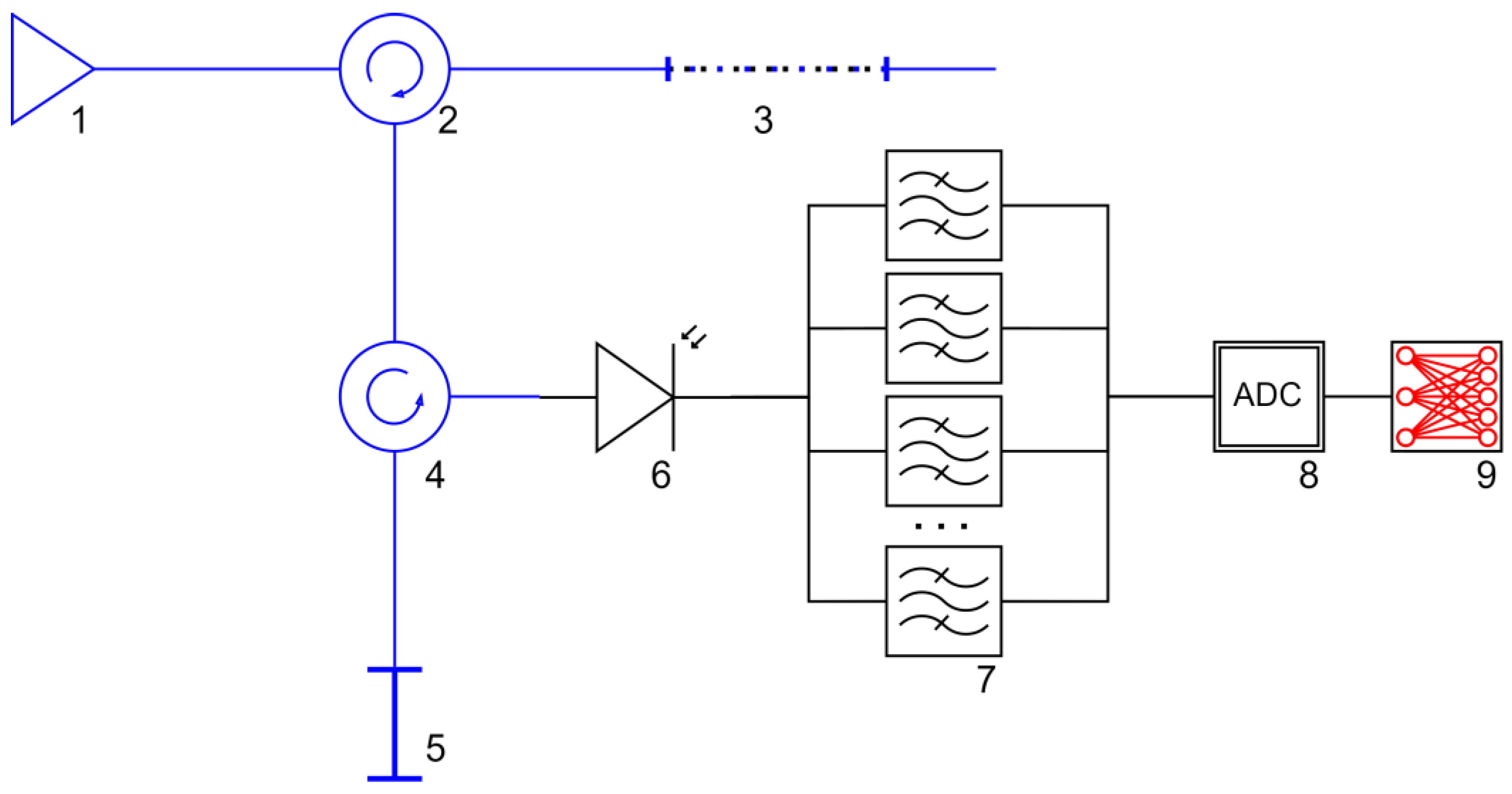
According to the proposed microwave photonic interrogation approach, the scheme of which is presented in Figure 1, the probing of the FPI reflection spectrum is carried out by an optical frequency comb including five–seven optical spectral components in the optical part of the spectrum with a step of 5–10 GHz (40–80 pm) and full width at half height up to 30–35 GHz (240–280 pm). The considered wavelength range of the FPI reflection spectrum is from 1520 nm to 1595 nm. The optical frequency comb can be formed using a wideband optical source (denoted as 1 in Figure 1), the radiation from which is reflected from the superstructured fiber Bragg grating 3 (described in detail in Section 3.3) and directed to the Fabry–Perot interferometer through the circulators 2 and 4.

The signal reflected from the FPI is directed to the photodetector through the circulator 4. On the photodetector, as on the element with a quadratic transfer characteristic, the cross-beating of all frequency components forming the optical frequency comb will be formed, and the frequency of beating components will be a multiple of the frequency spacing of the optical comb. The amplitude of the beating components is a multiple of the product of the amplitudes of the probing components of the optical frequency comb and the Fabry–Perot reflection spectrum. The flat shift of the comb spectrum leads to a change in the resulting amplitudes of the probing radiation and, as a consequence, in the amplitudes of the beating signal at the photodetector’s output. The beating signal is filtered using seven bandpass filters, the number of which corresponds to the number of the considered beating components, and is processed by the analog-to-digital converter 8. The obtained data is processed in the ANN-based unit 9 defining the measured value of temperature. Such a microwave photonic interrogation approach does not rely on the spectrometer, the resolution of which is limited by the CCD array, thereby enhancing the maximum achievable measurement resolution.

In the present work, the task was set to analyze the possibility and limits of applicability of determining the temperature of the Fabry–Perot sensing element by a set of amplitudes of the photodetector output signal obtained at multiple frequencies of the difference frequencies of the probing optical frequency comb.

3. Mathematical Model

The mathematical model of the FPI sensing element probing (a polymer film applied to the end of an optical fiber) includes the following: a model of the reflection spectrum of the Fabry–Perot interferometer, along with the dependence of its parameters on temperature; a model of the resulting spectrum of the probing optical frequency comb; a model of their interaction spectrum; a model of the electrical signal spectrum obtained at the photodetector; and a model of the amplitude detector at difference frequencies.

The mathematical model will enable the creation of a digital twin of the measurement conversion process of a fiber-optic sensor based on an FPI with a microwave photonic interrogation method at multiple difference frequencies. The susceptibility of the spectral response of the interferometer to environmental parameters, incorporated in the mathematical model, makes it possible to study the system at different values of temperature in the required range. The proposed mathematical model makes it possible to form a continuous set of training data for the artificial neural network.

3.1. Model of the Fabry–Perot Reflection Spectrum

The mathematical apparatus of scattering and transmission matrices was used to model the reflection spectrum of the Fabry–Perot interferometer [35]. In general, the reflection and transmission spectra of the Fabry–Perot interferometer are modelled by the product of three transmission matrices: (a) a discontinuous change in the propagation medium parameters (from the optical fiber core to the interferometer inner cavity); (b) a continuous medium of the interferometer inner cavity; and (c) a discontinuous change in the propagation medium parameters (from the interferometer inner cavity to the external medium). The scattering matrix of a continuous medium is a function of the radiation wavelength, permittivity, permeability and thickness of the medium:

$$S_{\mathrm{M}}=\left[\begin{array}{cc}0& e^{-j\cdot H\cdot \gamma }\\ e^{-j\cdot H\cdot \gamma }& 0\end{array}\right] ,$$

(1)

where

$$\gamma =\frac{\mathsf{\pi }}{\mathsf{\lambda }}\sqrt{2\mathrm{Re}\mathsf{\epsilon }\cdot \mathrm{Re}\mathsf{\mu }}\left(\sqrt{\sqrt{1-{\left(\frac{\mathrm{Im}\mathsf{\epsilon }}{\mathrm{Re}\mathsf{\epsilon }}\right)}^2}+1}-j\sqrt{\sqrt{1-{\left(\frac{\mathrm{Im}\mathsf{\epsilon }}{\mathrm{Re}\mathsf{\epsilon }}\right)}^2}-1}\right) ,$$

(2)

ε and μ are the permittivity and permeability of the solid medium, H is the thickness of the solid medium, and λ is the wavelength of radiation.

The scattering matrices of the discontinuity of the medium parameters at the boundaries of propagation media are a function of the permittivities and permeabilities of the media:

$$S_{\mathrm{J}}^{12}=\left[\begin{array}{cc}\frac{\sqrt{{\mathsf{\epsilon }}_1{\mathsf{\mu }}_2}-\sqrt{{\mathsf{\mu }}_1{\mathsf{\epsilon }}_2}}{\sqrt{{\mathsf{\mu }}_1{\mathsf{\epsilon }}_2}+\sqrt{{\mathsf{\epsilon }}_1{\mathsf{\mu }}_2}}& \frac{2\cdot \sqrt[4]{{\mathsf{\epsilon }}_1{\mathsf{\mu }}_1{\mathsf{\epsilon }}_2{\mathsf{\mu }}_2}}{\sqrt{{\mathsf{\mu }}_1{\mathsf{\epsilon }}_2}+\sqrt{{\mathsf{\epsilon }}_1{\mathsf{\mu }}_2}}\\ \frac{2\cdot \sqrt[4]{{\mathsf{\epsilon }}_1{\mathsf{\mu }}_1{\mathsf{\epsilon }}_2{\mathsf{\mu }}_2}}{\sqrt{{\mathsf{\mu }}_1{\mathsf{\epsilon }}_2}+\sqrt{{\mathsf{\epsilon }}_1{\mathsf{\mu }}_2}}& \frac{\sqrt{{\mathsf{\epsilon }}_1{\mathsf{\mu }}_2}-\sqrt{{\mathsf{\mu }}_1{\mathsf{\epsilon }}_2}}{\sqrt{{\mathsf{\mu }}_1{\mathsf{\epsilon }}_2}+\sqrt{{\mathsf{\epsilon }}_1{\mathsf{\mu }}_2}}\end{array}\right] , S_{\mathrm{J}}^{23}=\left[\begin{array}{cc}\frac{\sqrt{{\mathsf{\epsilon }}_2{\mathsf{\mu }}_3}-\sqrt{{\mathsf{\mu }}_2{\mathsf{\epsilon }}_3}}{\sqrt{{\mathsf{\mu }}_2{\mathsf{\epsilon }}_3}+\sqrt{{\mathsf{\epsilon }}_2{\mathsf{\mu }}_3}}& \frac{2\cdot \sqrt[4]{{\mathsf{\epsilon }}_2{\mathsf{\mu }}_2{\mathsf{\epsilon }}_3{\mathsf{\mu }}_3}}{\sqrt{{\mathsf{\mu }}_2{\mathsf{\epsilon }}_3}+\sqrt{{\mathsf{\epsilon }}_2{\mathsf{\mu }}_3}}\\ \frac{2\cdot \sqrt[4]{{\mathsf{\epsilon }}_2{\mathsf{\mu }}_2{\mathsf{\epsilon }}_3{\mathsf{\mu }}_3}}{\sqrt{{\mathsf{\mu }}_2{\mathsf{\epsilon }}_3}+\sqrt{{\mathsf{\epsilon }}_2{\mathsf{\mu }}_3}}& \frac{\sqrt{{\mathsf{\epsilon }}_2{\mathsf{\mu }}_3}-\sqrt{{\mathsf{\mu }}_2{\mathsf{\epsilon }}_3}}{\sqrt{{\mathsf{\mu }}_2{\mathsf{\epsilon }}_3}+\sqrt{{\mathsf{\epsilon }}_2{\mathsf{\mu }}_3}}\end{array}\right] ,$$

(3)

where ε₁ and μ₁ are the permittivity and permeability of the optical fiber, ε₂ and μ₂ are the permittivity and permeability of the Fabry–Perot interferometer cavity (polymer film), and ε₃ and μ₃ are the permittivity and permeability of the external medium.

The scattering matrices S are transformed into the transmission matrix T and back by operators of the form

$$\overleftrightarrow{\mathbf{T}}\left(S\right)=\frac{1}{S_{2,1}}\left(\begin{array}{cc}{S}_{2,1}{S}_{1,2}-S_{1,1}{S}_{2,2}& S_{1,1}\\ -S_{2,2}& 1\end{array}\right),\overleftrightarrow{\mathbf{S}}\left(T\right)=\frac{1}{T_{2,2}}\left(\begin{array}{cc}{T}_{1,2}& T_{1,1}{T}_{2,2}-T_{1,2}{T}_{2,1}\\ 1& T_{2,1}\end{array}\right).$$

(4)

The Fabry–Perot transmission matrix is the result of successive multiplication of the transmission matrices of the partition boundaries and the internal cavity of the interferometer (continuous medium) and is a function depending on the radiation wavelength, dielectric and magnetic permeability of the media, and cavity length:

$$T^{\mathrm{FP}}=T_{\mathrm{J}}^{12}\times T_{\mathrm{M}}^2\times T_{\mathrm{J}}^{23} .$$

(5)

In (5), the lower index defines the transmission matrix (“J”—discontinuous change of parameters, “M”—continuous medium), the upper index of the matrix “J” indicates the direction of radiation transition from the i-th layer to the (i + 1)-th layer, and the upper index of the matrix “M” defines the parameters of the interferometer cavity.

The S^FP scattering matrix of the Fabry–Perot interferometer is obtained by inverse transformation of the T^FP transmission matrix by (4):

$$S^{\mathrm{FP}}=\frac{1}{{\left(T^{\mathrm{FP}}\right)}_{2,2}}\left(\begin{array}{cc}{\left(T^{\mathrm{FP}}\right)}_{1,2}& ‖T^{\mathrm{FP}}‖\\ 1& {\left(T^{\mathrm{FP}}\right)}_{2,1}\end{array}\right) .$$

(6)

The (S^FP)_1,1 element of the resulting scattering matrix defines the dependence of the Fabry–Perot interferometer reflection coefficient for radiation directed into it from the optical fiber side; (S^FP)_2,2 is the reflection coefficient from the external boundary for radiation directed from the external medium; (S^FP)_1,2 is the transmittance coefficient for radiation directed from the optical fiber side; and (S^FP)_2,1 is the transmittance coefficient for radiation directed from the external medium side.

In general, all reflection and transmission coefficients are functions of the wavelength, of the dielectric and magnetic permeabilities of all media and of the length of the internal cavity of the interferometer.

3.2. Controlling the Parameters of the Fabry–Perot Interferometer with Temperature Changes

A change in ambient temperature directly affects all seven parameters of the interferometer, namely the dielectric and magnetic permeabilities of the three media as well as the length of the interferometer’s internal cavity. As our previous studies have shown, if the propagation medium is a quartz fiber, the interferometer inner cavity is a polymer (dielectric), and the external medium is air; then the temperature effect on the Fabry–Perot spectrum shift has a change only in the dielectric permittivity and the length of the interferometer inner cavity [34].

To model the temperature change of the interferometer inner cavity, the linear dependence of its dielectric permittivity and length on the temperature change was used:

$${\mathsf{\epsilon }}_2\left(T\right)={\mathsf{\epsilon }}_{20}\left(1+K_{\mathsf{\epsilon }2}\cdot \Delta T\right), H\left(T\right)=H_0\left(1+\mathsf{\alpha }\cdot \Delta T\right),$$

(7)

where K_ε2 is the temperature coefficient of dielectric constant of the interferometer inner cavity, α is the coefficient of thermal expansion of the polymer film, ε₂₀ is the value of dielectric constant, and H₀ is the length of the interferometer inner cavity at the reference temperature. The permittivity of the optical fiber ε₁ also has a linear temperature dependence similar to (7) with the temperature coefficient K_ε1.

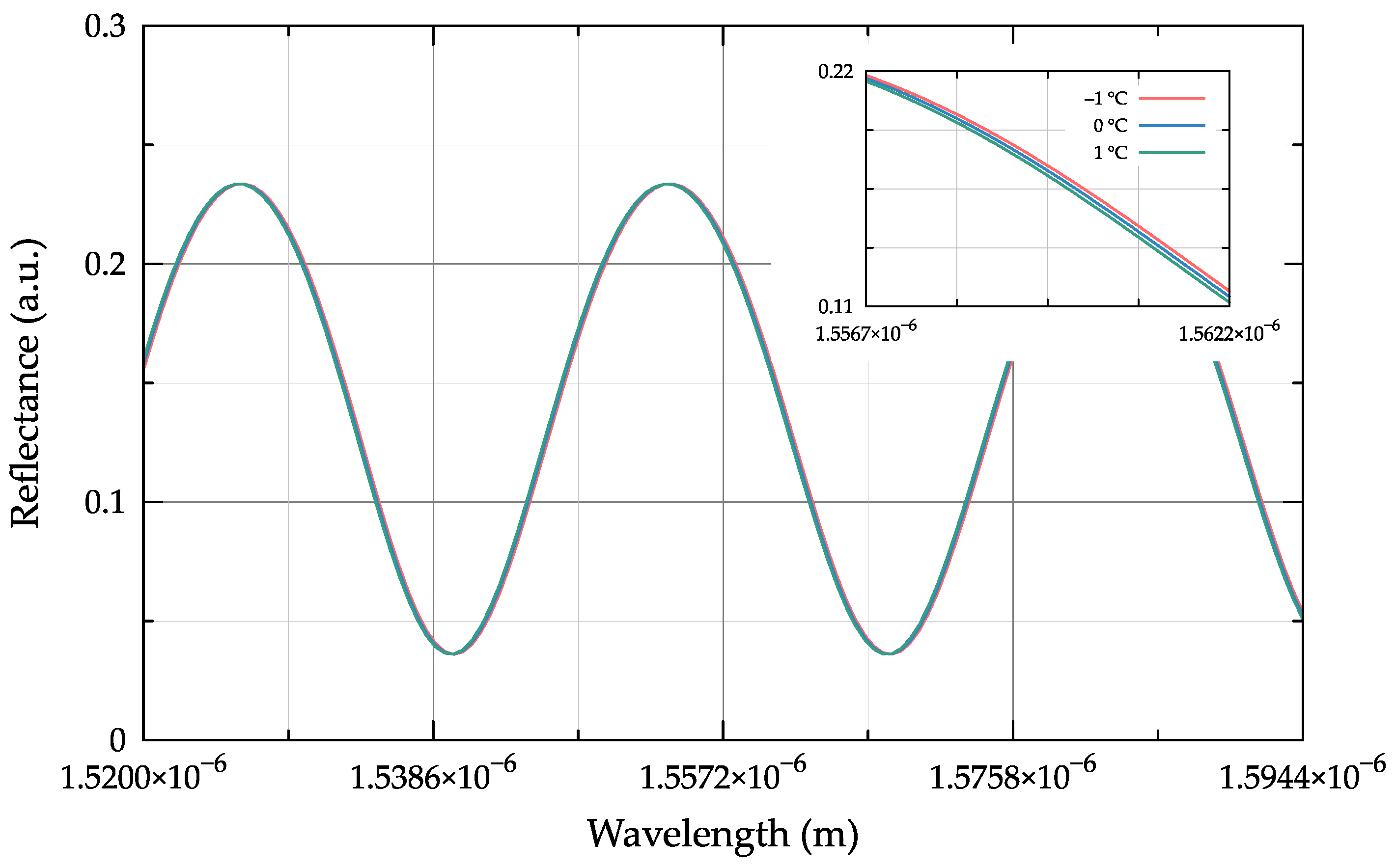
The modelling result of the Fabry–Perot interferometer reflection spectrum obtained at ±1 °C temperature change is shown in Figure 2 (data obtained at ε₁ = 2.1556, μ₁ = 1.0, ε₂₀ = 4.2025, μ₂ = 1.0, ε₃ = 1.0, μ₃ = 1.0, H₀ = 21 μm, K_ε2 = 15 × 10⁻⁶ T⁻¹, K_ε1 = 8.6 × 10⁻⁶ T⁻¹, α = 1 × 10⁻⁶ T⁻¹).

3.3. Probing Radiation

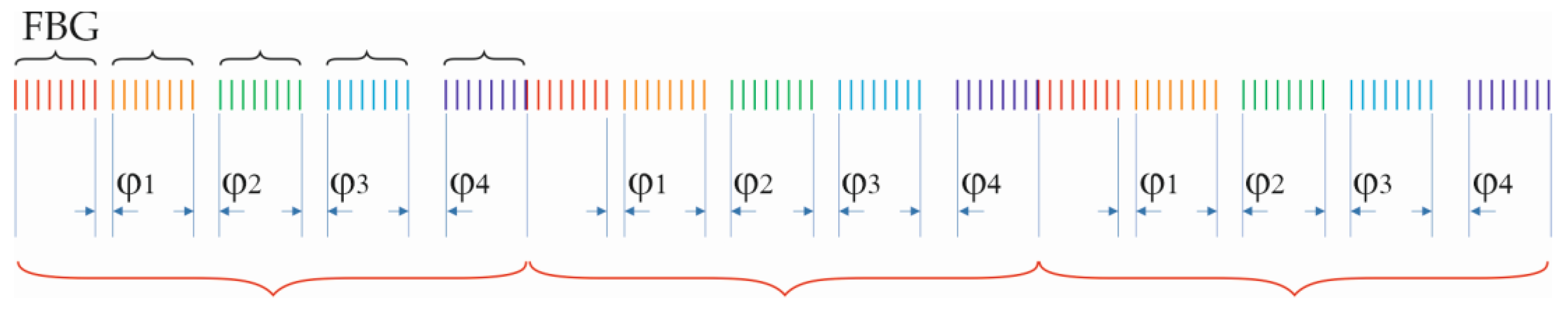
Optical frequency comb or spectral comb is an optical radiation, the spectrum of which consists of discrete and evenly spaced spectral lines. Optical oscillators are capable of generating several evenly spaced optical carriers with a minimum number of components. Another method of optical frequency comb formation can be implemented based on a superstructured array of homogeneous weakly reflective Bragg fiber gratings with phase shifts between them. The superstructure consists of a periodically repeating nested structure, which is a combination of homogeneous weakly reflecting Bragg gratings arranged with phase inhomogeneities of the form

$$\left\{{\mathsf{\phi }}_i\right\}=2\mathsf{\pi }\frac{i}{n} , i\in \mathbb{N},$$

(8)

determining the phase shift between the gratings, where n is the number of partitions of the full circle [0, 2π] into sections φ_i. An example of a superstructure scheme consisting of three separate structures, each formed from five homogeneous fiber Bragg gratings, is shown in Figure 3. The red curly braces in the figure denote the structures, and the black curly braces denote the homogeneous Bragg fiber gratings; φ_i denotes the phase shifts configured by (8).

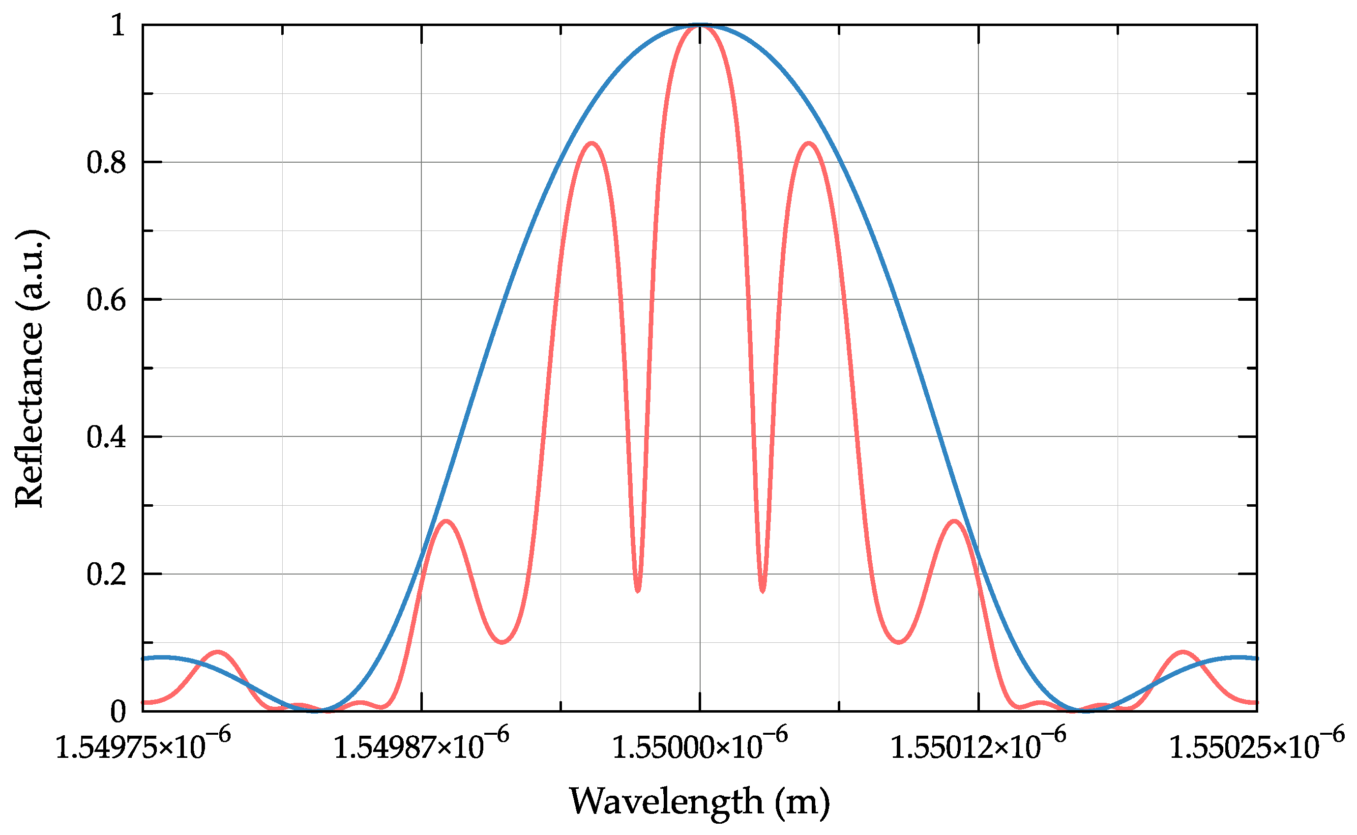
This approach to structure creation allows to form a frequency comb in the optical range and at the same time significantly increase the reflectivity of its individual components, as shown in Figure 4 obtained via numerical simulation using the transfer matrix method. The model was implemented under the assumption of the structure implementation within a single-mode optical fiber with a core refractive index of 1.4586, induced refractive index of 1 × 10⁻⁴, n = 4, homogeneous segment length of 5 mm and grating period of 5.3129 × 10⁻⁷ m.

The envelope of the optical frequency comb spectrum coincides with the reflection spectrum of the Bragg fiber array with a length corresponding to the length of one homogeneous segment, as shown in Figure 4. Varying the number of homogeneous segments in the structure, as well as the number of structures in the superstructure, allows controlling the number of frequency components in the reflection spectrum while maintaining the total length of the structure. Thus, for example, at n = 1 (φ_i = 0) a single-frequency structure is formed; at n = 1 (φ_i = π), a two-frequency structure with a difference frequency Ω between the components; at n = 2 (φ_i = 0, π), a four-frequency comb with a difference frequency Ω/2; at n = 3 (φ_i = 0, 2π/3, 4π/3), an eight-frequency comb with a difference frequency Ω/3; etc.

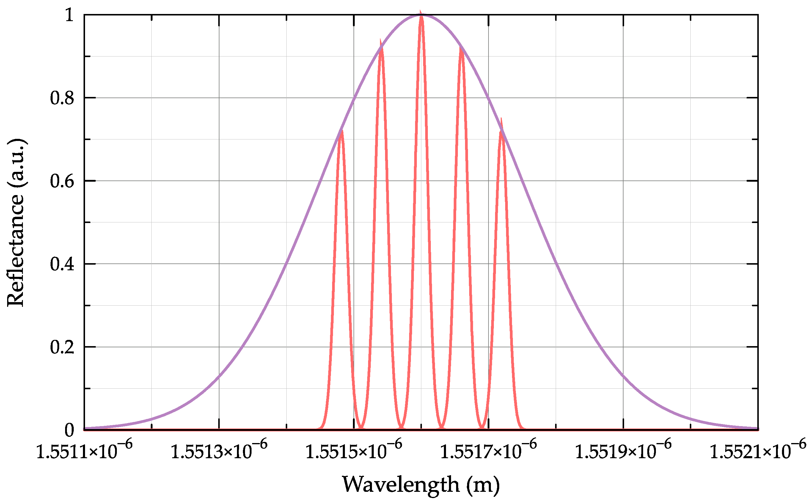
Based on the analysis of works devoted to the implementation of optical frequency combs [36,37,38], we can conclude that, in general, the spectrum of an optical frequency comb can be considered a set of evenly spaced spectral components with a common envelope. In the present work, we used a mathematical model of the optical frequency comb spectrum, each component of which is described by a normal distribution function, with a common envelope also described by a normal distribution function. This description of the optical frequency comb spectrum allows controlling both the number of spectral components and the distance between them, as well as the shape and parameters of the spectral components and the common envelope. The mathematical model also allows replacing the normal distribution function, for example, by a Lorentz function or similar. An example of an optical frequency comb spectrum with a spectral width of 5 nm, a total number of optical components equal to 5, a center wavelength of λ = 1551.8 nm, and a common envelope with σ = 1.1 × 10⁻¹⁰ is shown in Figure 5.

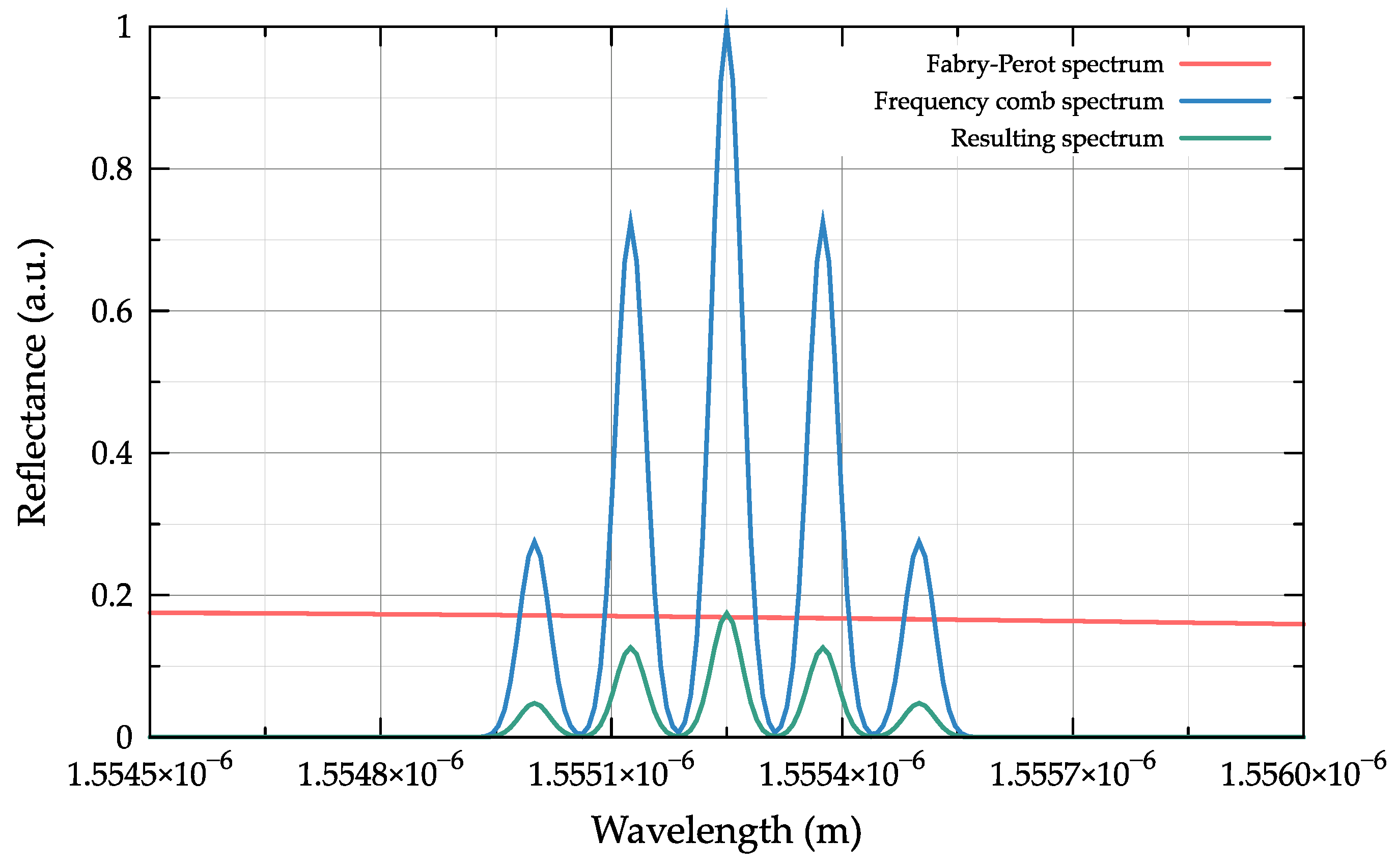
The interaction spectrum of the probing radiation and the Fabry–Perot interferometer is modelled by multiplication at the same wavelengths (frequencies) of the spectra of the interferometer and the optical frequency comb, as shown in Figure 6.

The displacement of the Fabry–Perot interferometer spectrum at temperature change entails a change in the amplitudes of the spectral components of the probing study of the optical frequency comb, the spectral position of which is assumed to be stabilized at the middle of the linear section of the spectral response of the interferometer.

3.4. Photodetector

A photodetector is a nonlinear quadratic element, the output current of which is proportional to the square of the modulus of the optical radiation incident on it. As a result, on the photodetector there are cross-beatings of all components of the optical frequency comb radiation falling on it. The spectrum of radiation falling on the photodetector is modelled by a linear discrete spectrum, the detail of discretization of which can be chosen as practically any. In practice, the sampling frequency is determined by the criterion of model signal correspondence to the real one. The spectrum of the signal arriving at the photodetector can be described as a discrete set of amplitudes {A_k}, k = 0, N; hence, the light flux can be described as a set of monochromatic emissions at discrete frequencies:

$$Z\left(t\right)={\displaystyle \sum _{k=0}^N{A}_k\cdot e^{j\cdot \frac{2\mathsf{\pi }c}{{\mathsf{\lambda }}_k}\cdot t}}={\displaystyle \sum _{k=0}^N{A}_k\cdot e^{j\cdot {\mathsf{\omega }}_k\cdot t}},$$

(9)

where N is the number of spectrum discretization points, A_k is the spectrum amplitude at wavelength λ_k = λ₀ + k·Δλ, Δλ is the discretization step of the spectrum wavelength, c is the speed of light, ω_k = 2π·c/λ_k is the frequency, and Δω = 2π·c∙Δλ/(λ²) is the frequency discretization step. The output current of the photodetector is proportional to the square of the modulus of the light flux incident on it:

$$P\left(t\right)\sim {\left|Z\left(t\right)\right|}^2=Z\left(t\right)\overline{Z\left(t\right)}={\displaystyle \sum _{i=0}^N{A}_i\times e^{j{\mathsf{\omega }}_{i}t}}\overline{{\displaystyle \sum _{k=0}^N{A}_k\times e^{j{\mathsf{\omega }}_{k}t}}}$$

(10)

If we open the brackets, we obtain

$$P\left(t\right)\sim {\displaystyle \sum _{i=0}^N{A}_i^2}+2\cdot {\displaystyle \sum _{n=1}^{N-1}{\displaystyle \sum _{i=0}^{N-n}{A}_i\cdot A_{i+n}\cdot \cos \left(n\cdot \Delta \mathsf{\omega }\cdot t\right)}}.$$

(11)

Consequently, the photodetector output current at frequency Ω_n = n·Δω is proportional to the sum of products of all amplitudes whose difference frequency coincides with the frequency Ω_n:

$$P_n\left({\mathsf{\Omega }}_n\right)\sim 2\cdot {\displaystyle \sum _{n=1}^N{\displaystyle \sum _{i=0}^{N-n}{A}_i\cdot A_{i+n}}}.$$

(12)

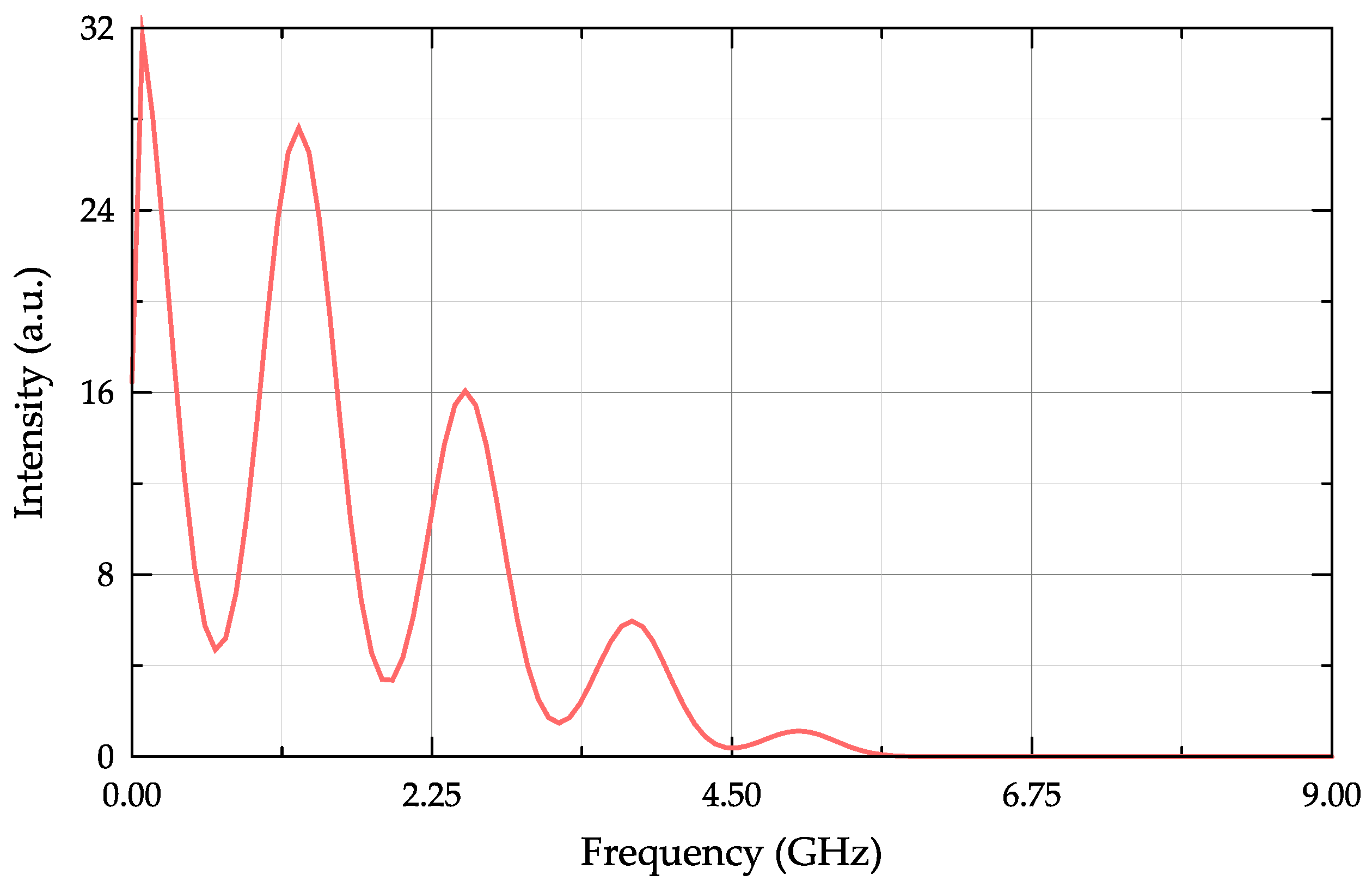
The increase in the number of points of modelling the reflection spectrum and the photodetector output current spectrum is directly proportional to the approximation accuracy and inversely proportional to the modelling time, and within the model any number of points in the spectra can be chosen, with it being an adjustable parameter. An example of the photodetector spectrum model corresponding to the presented reflectance spectra of the Fabry–Perot interferometer and the probing radiation shown in the previous figures is presented in Figure 7.

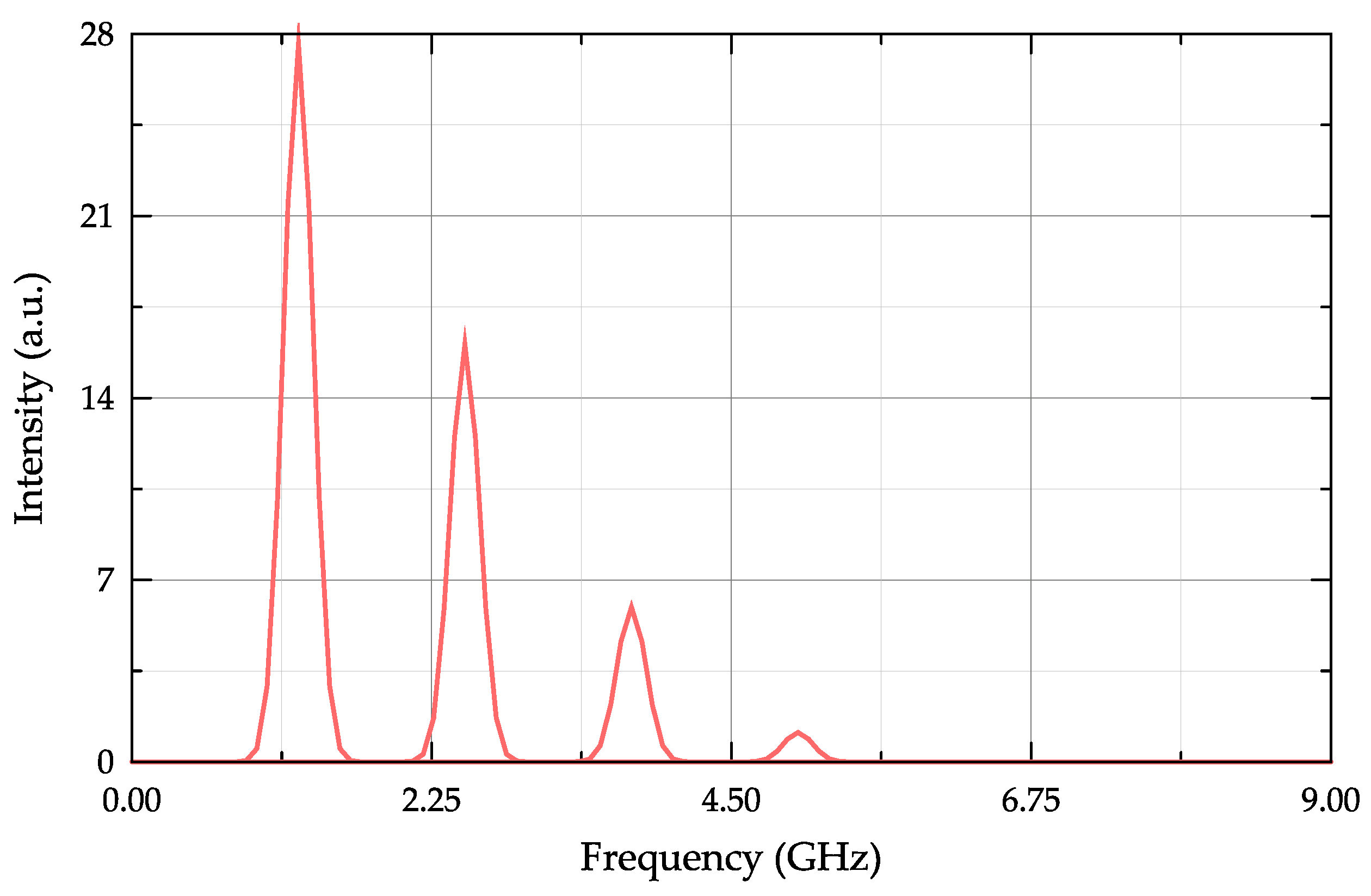
The microwave photonic method involves the analysis of the photodetector output signal at the difference frequencies of the optical frequency comb, which correspond to the maximum peaks of the photodetector output current peaks. To select the amplitudes of the photodetector output current at differential frequencies of the optical frequency comb, it is necessary to filter the output current signal at multiple frequencies of the comb step. The model uses a bandpass frequency filter whose amplitude–frequency response is described by a normal distribution function. An example of the resulting spectrum, when selecting frequencies by the bandpass filter, is shown in Figure 8.

The parameters of the frequency bandpass filter at the output of the photodetector are flexibly adjustable, which allows us to use the model of this tool to build various signal processing tools. Theoretically, it would be possible to choose a bandpass filter with an arbitrary frequency response, but, as numerical experiments have shown, the influence of its shape is negligible.

4. Data Format

When starting work on this topic, the authors were guided by the hypothesis that the position of the Fabry–Perot reflection spectrum can be put in unambiguous correspondence from the mutual ratio of amplitudes obtained by microwave photonic probing of the interferometer optical frequency comb with their separation at differential frequencies. A change in the external temperature leads to a change in the dielectric permittivity and film thickness of the Fabry–Perot interferometer and, as has already been shown, to a shift in the spectrum, and the shift in the spectrum, in turn, will lead to a change in the amplitudes of the probing signal and, as a consequence, to a change in the amplitudes of the beats of the photodetector output current at differential frequencies of the optical frequency comb. Thus, the task was to unambiguously compare the ratio of the photodetector output current amplitudes at differential frequencies to the temperature value.

To train the artificial neural network, microwave photonic processing data were generated for temperature values varying in the range from −15 to +15 °C with a discrete step of ΔT = 0.001 °C. The small data discretization step is due to the need to obtain a large amount of data required for training the artificial neural network in order to improve its accuracy. This resulted in a marked-up set of 30,100 data which were normalized into a dimensionless interval [0; 1] for input and output data, finally giving a normalized set of input and output data for training.

5. Artificial Neural Network Model

In general, to build an artificial neural network corresponding to the task at hand, we need a fully connected ANN designed for processing one-dimensional signals [39,40,41], having at the input the number of neurons per unit less than the number of frequency components of the optical frequency comb (equal to the number of frequencies of cross-beats of the comb components) and the output (last) layer in the network must contain one neuron that determines the temperature value. There are no special recommendations for selecting the number of hidden (computational) layers and neurons in them; various configurations have been tested in this work.

The logistic activation function was used for training. The accuracy of the model performance was assessed simultaneously by two parameters: mean absolute error, MAE, and mean relative error, MRPE, which were calculated using the formulas

$$MAE=\frac{1}{M}{\displaystyle \sum _{i=1}^M\left|y_i-p_i\right|} , MRPE=\frac{1}{M}{\displaystyle \sum _{i=1}^M\frac{\left|y_i-p_i\right|}{y_i}\cdot 100 \%} ,$$

(13)

where M is the number of data in the dataset, y_i is the actual value, and p_i is the predicted value for the i-th dataset. Several of the tested configurations of the ANN are listed in

Table 1. Error values for various configurations of ANN.

No. of ANN	No. of Hidden Layers	No. of Neurons in Each Hidden Layer	MAE, °C
(1)	1	50	4
(2)	1	200	3.5
(3)	2	50/20	1.5
(4)	2	100/50	1
(5)	3	50/20/20	0.5
(6)	3	150/100/50	0.48
(7)	4	100/100/50/50	0.39
(8)	4	700/500/300/200	0.15
(9)	4	1500/1000/500/400	0.12

with the corresponding MAE values obtained in the temperature range from −15 to +15 °C. In all of the configurations, the input layer consisted of four neurons, and the output layer included one neuron.

The configuration No. 8 from Table 1 was used in the current study, which is a fully connected ANN corresponding to probing with an optical frequency comb containing five frequency components, the input layer of which consisted of four neurons, followed sequentially by hidden layers containing 700, 500, 300 and 200 neurons, respectively. The output layer consisted of one neuron. The activation function for all hidden layers was LeakyReLU with a negative slope coefficient of 0.3, while for the output layer tanh function was used. The ANN was implemented using Python 3.11 with the TensorFlow library.

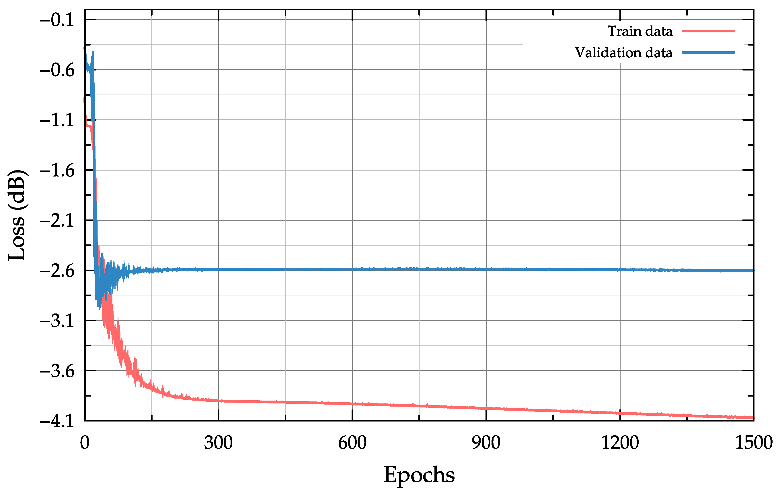
As part of the input data, as required by the training algorithms, the labelled dataset was divided into a training dataset (90%) and a control dataset (10%). The training dataset was used directly to adjust the weights, while the control dataset was used to determine the accuracy of model performance between training iterations and was not used to adjust the weights. Already after 1500 epochs of training, the value of the loss function did not exceed 0.001, as shown in Figure 9.

Values of absolute and relative errors of temperature determination are given in

Table 2. Error values for temperature determination in various ranges for the developed ANN.

Range, °C	MAE, °C	MRPE, %
from −15 to +15	0.14698	2.508
from −14 to +14	0.0866	2.2023
from −13 to +13	0.064	2.1564
from −12 to +12	0.0467	2.1547
from −11 to +11	0.0291	2.1605
from −10 to +10	0.01859	2.2488

below.

The obtained data show that the trained artificial neural network model has the maximum error at the largest verifiable range, and as the range decreases, the error value decreases significantly to 0.08 °C, which is good accuracy.

6. Conclusions

According to the results of the work, the following set of conclusions can be made. Firstly, the empirical method was used to confirm the assumption that the position of the Fabry–Perot reflection spectrum can be unambiguously compared with the amplitudes of the signal obtained by microwave photonic probing of the Fabry–Perot interferometer by an optical frequency comb with separation of the amplitudes of the photodetector output current at differential frequencies. Secondly, the prospect of using the Fabry–Perot end-face interferometer, implemented on the end of an optical fiber in the form of a thin polymer film as a temperature sensor, which can be interrogated by microwave photonic methods, is confirmed. Thirdly, it is shown that due to the choice of the network configuration and probing radiation, it is possible to achieve an accuracy of temperature determination from 0.146 to 0.018 °C, and a reduction in the range of temperature variation by two degrees leads to a reduction in the average absolute error of temperature determination by 1.75 times.

In conclusion, the combination of artificial intelligence algorithms with microwave photonic interrogation methods has great potential in the field of fiber-optic sensing. The combination of microwave photonic methods together with artificial intelligence algorithms can potentially produce more accurate results with higher frequency and at lower cost. The proposed innovative approach can significantly contribute to the development of high-precision measurement systems.

References

- Capmany, J.; Novak, D. Microwave Photonics Combines Two Worlds. Nat. Photonics 2007, 1, 319–330. [Google Scholar] [CrossRef]
- Minasian, R.A. Photonic Signal Processing of Microwave Signals. IEEE Trans. Microw. Theory Tech. 2006, 54, 832–846. [Google Scholar] [CrossRef]
- Seeds, A.J. Microwave Photonics. IEEE Trans. Microw. Theory Tech. 2002, 50, 877–887. [Google Scholar] [CrossRef]
- Yamaoka, S.; Diamantopoulos, N.-P.; Nishi, H.; Nakao, R.; Fujii, T.; Takeda, K.; Hiraki, T.; Tsurugaya, T.; Kanazawa, S.; Tanobe, H.; et al. Directly Modulated Membrane Lasers with 108 GHz Bandwidth on a High-Thermal-Conductivity Silicon Carbide Substrate. Nat. Photonics 2021, 15, 28–35. [Google Scholar] [CrossRef]
- Rostokin, I.N.; Fedoseeva, E.V.; Rostokin, E.A.; Kariaev, V.V.; Morozov, O.G.; Sakhabutdinov, A.Z.; Nureev, I.I.; Morozov, G.A. Design Features of Microwave Photonic Radars. In Proceedings of the XVII International Scientific and Technical Conference “Optical Technologies for Telecommunications”; Andreev, V.A., Bourdine, A.V., Burdin, V.A., Morozov, O.G., Sultanov, A.H., Eds.; SPIE: Cergy, France, 2020; Volume 11516. [Google Scholar]
- Ivanov, A.; Morozov, O.; Sakhabutdinov, A.; Kuznetsov, A.; Nureev, I. Photonic-Assisted Receivers for Instantaneous Microwave Frequency Measurement Based on Discriminators of Resonance Type. Photonics 2022, 9, 754. [Google Scholar] [CrossRef]
- Wang, D.; Zhang, X.; An, X.; Ding, Y.; Li, J.; Dong, W. Microwave Frequency Measurement System Using Fixed Low Frequency Detection Based on Photonic Assisted Brillouin Technique. IEEE Trans. Instrum. Meas. 2023, 72, 1–10. [Google Scholar] [CrossRef]
- Kim, D.-W.; Kodama, S.; Sekiguchi, H.; Park, D.-W. Formation Phenomena of Iron Oxide-Silica Composite in Microwave Plasma and DC Thermal Plasma. Adv. Powder Technol. 2018, 29, 168–179. [Google Scholar] [CrossRef]
- Agliullin, T.; Il’In, G.; Kuznetsov, A.; Misbakhov, R.; Misbakhov, R.; Morozov, G.; Morozov, O.; Nureev, I.; Sakhabutdinov, A. Addressed Fiber Bragg Structures: Principles and Applications Overview. Preprints 2022, 2022100109. [Google Scholar] [CrossRef]
- Ricchiuti, A.L.; Barrera, D.; Sales, S.; Thévenaz, L.; Capmany, J. Long Weak FBG Sensor Interrogation Using Microwave Photonics Filtering Technique. IEEE Photonics Technol. Lett. 2014, 26, 2039–2042. [Google Scholar] [CrossRef]
- Xu, O.; Zhang, J.; Yao, J. High Speed and High Resolution Interrogation of a Fiber Bragg Grating Sensor Based on Microwave Photonic Filtering and Chirped Microwave Pulse Compression. Opt. Lett. 2016, 41, 4859–4862. [Google Scholar] [CrossRef]
- Nasybullin, A.R.; Anfinogentov, V.I.; Lipatnikov, K.A.; Smirnov, S.V. Multi-Sensor Temperature and Humidity Measuring System for Technological Process of Organic Livestock Waste Microwave Treatment Monitoring. In Proceedings of the 2021 Wave Electronics and Its Application in Information and Telecommunication Systems (WECONF), St. Petersburg, Russia, 31 May–4 June 2021. [Google Scholar]
- Jin, Y.; Dong, X.; Gong, H.; Shen, C. Refractive-Index Sensor Based on Tilted Fiber Bragg Grating Interacting with Multimode Fiber. Microw. Opt. Technol. Lett. 2010, 52, 1375–1377. [Google Scholar] [CrossRef]
- Roriz, P.; Silva, S.; Frazão, O.; Novais, S. Optical Fiber Temperature Sensors and Their Biomedical Applications. Sensors 2020, 20, 2113. [Google Scholar] [CrossRef]
- A Review on Capacitive-Type Sensor for Measurement of Height of Liquid Level—Brajesh Kumar, G Rajita, Nirupama Mandal. 2014. Available online: https://journals.sagepub.com/doi/full/10.1177/0020294014546943 (accessed on 12 February 2024).
- Sensors|Free Full-Text|Design and Implementation of an Intrinsically Safe Liquid-Level Sensor Using Coaxial Cable. Available online: https://www.mdpi.com/1424-8220/15/6/12613 (accessed on 12 February 2024).
- Singh, A.; Mittal, S.; Das, M.; Saharia, A.; Tiwari, M. Optical Biosensors: A Decade in Review. Alex. Eng. J. 2023, 67, 673–691. [Google Scholar] [CrossRef]
- Huang, Y.; Guo, T.; Tian, Z.; Yu, B.; Ding, M.; Li, X.; Guan, B.-O. Nonradiation Cellular Thermometry Based on Interfacial Thermally Induced Phase Transformation in Polymer Coating of Optical Microfiber. ACS Appl. Mater. Interfaces 2017, 9, 9024–9028. [Google Scholar] [CrossRef]
- Abdeljaber, O.; Avci, O.; Kiranyaz, M.S.; Boashash, B.; Sodano, H.; Inman, D.J. 1-D CNNs for Structural Damage Detection: Verification on a Structural Health Monitoring Benchmark Data. Neurocomputing 2018, 275, 1308–1317. [Google Scholar] [CrossRef]
- Avci, O.; Abdeljaber, O.; Kiranyaz, S.; Inman, D. Convolutional Neural Networks for Real-Time and Wireless Damage Detection. In Proceedings of the Dynamics of Civil Structures; Pakzad, S., Ed.; Springer International Publishing: Cham, Switzerland, 2020; Volume 2, pp. 129–136. [Google Scholar]
- Cha, Y.-J.; Choi, W.; Büyüköztürk, O. Deep Learning-Based Crack Damage Detection Using Convolutional Neural Networks: Deep Learning-Based Crack Damage Detection Using CNNs. Comput. Aided Civ. Infrastruct. Eng. 2017, 32, 361–378. [Google Scholar] [CrossRef]
- Cochocki, A.; Unbehauen, R. Neural Networks for Optimization and Signal Processing, 1st ed.; John Wiley & Sons, Inc.: Hoboken, NJ, USA, 1993; ISBN 978-0-471-93010-5. [Google Scholar]
- Eren, L. Bearing Fault Detection by One-Dimensional Convolutional Neural Networks. Math. Probl. Eng. 2017, 2017, e8617315. [Google Scholar] [CrossRef]
- Jiang, H.; Zeng, Q.; Chen, J.; Qiu, X.; Liu, X.; Chen, Z.; Miao, X. Wavelength Detection of Model-Sharing Fiber Bragg Grating Sensor Networks Using Long Short-Term Memory Neural Network. Opt. Express 2019, 27, 20583. [Google Scholar] [CrossRef]
- Yang, W.; Tan, Z.; Yu, S.; Ren, Y.; Pan, R.; Yu, X. A Highly Sensitive Optical Fiber Sensor Enables Rapid Triglycerides-Specific Detection and Measurement at Different Temperatures Using Convolutional Neural Networks. Int. J. Biol. Macromol. 2024, 256, 128353. [Google Scholar] [CrossRef]
- Lu, H.; Fang, N.; Wang, L. Signal Identification Based on Modified Filter Bank Feature and Generalized Regression Neural Network for Optical Fiber Perimeter Sensing. Opt. Fiber Technol. 2022, 72, 102993. [Google Scholar] [CrossRef]
- Ren, L.; Zhao, J.; Zhou, Y.; Li, L.; Zhang, Y. Artificial Neural Network-Assisted Optical Fiber Sensor for Accurately Measuring Salinity and Temperature. Sens. Actuators Phys. 2024, 366, 114958. [Google Scholar] [CrossRef]
- Djurhuus, M.S.E.; Werzinger, S.; Schmauss, B.; Clausen, A.T.; Zibar, D. Machine Learning Assisted Fiber Bragg Grating-Based Temperature Sensing. IEEE Photonics Technol. Lett. 2019, 31, 939–942. [Google Scholar] [CrossRef]
- Liu, T.; Chen, Y.; Han, Q.; Liu, F.; Yao, Y. Sensor Based on Macrobent Fiber Bragg Grating Structure for Simultaneous Measurement of Refractive Index and Temperature. Appl. Opt. 2016, 55, 791. [Google Scholar] [CrossRef]
- Agliullin, T.; Anfinogentov, V.; Misbakhov, R.; Morozov, O.; Nasybullin, A.; Sakhabutdinov, A.; Valeev, B. Application of Neural Network Algorithms for Central Wavelength Determination of Fiber Optic Sensors. Appl. Sci. 2023, 13, 5338. [Google Scholar] [CrossRef]
- Aref, S.H.; Latifi, H.; Zibaii, M.I.; Afshari, M. Fiber Optic Fabry–Perot Pressure Sensor with Low Sensitivity to Temperature Changes for Downhole Application. Opt. Commun. 2007, 269, 322–330. [Google Scholar] [CrossRef]
- Chen, X.; Chardin, C.; Makles, K.; Caër, C.; Chua, S.; Braive, R.; Robert-Philip, I.; Briant, T.; Cohadon, P.-F.; Heidmann, A.; et al. High-Finesse Fabry–Perot Cavities with Bidimensional Si3N4 Photonic-Crystal Slabs. Light Sci. Appl. 2017, 6, e16190. [Google Scholar] [CrossRef]
- Chen, Z.; Xiong, S.; Gao, S.; Zhang, H.; Wan, L.; Huang, X.; Huang, B.; Feng, Y.; Liu, W.; Li, Z. High-Temperature Sensor Based on Fabry-Perot Interferometer in Microfiber Tip. Sensors 2018, 18, 202. [Google Scholar] [CrossRef]
- Hussein, S.M.R.H.; Sakhabutdinov, A.Z.; Morozov, O.G.; Anfinogentov, V.I.; Tunakova, J.A.; Shagidullin, A.R.; Kuznetsov, A.A.; Lipatnikov, K.A.; Nasybullin, A.R. Applicability Limits of the End Face Fiber-Optic Gas Concentration Sensor, Based on Fabry-Perot Interferometer. Karbala Int. J. Mod. Sci. 2022, 8, 339–355. [Google Scholar] [CrossRef]
- Német, N.; White, D.; Kato, S.; Parkins, S.; Aoki, T. Transfer-Matrix Approach to Determining the Linear Response of All-Fiber Networks of Cavity-QED Systems. Phys. Rev. Appl. 2020, 13, 064010. [Google Scholar] [CrossRef]
- Hammadi, Y.I. Design and Analysis of Optical Frequency Comb Generator Employing EAM. In Proceedings of the 2022 International Conference on Computer Science and Software Engineering (CSASE), Duhok, Iraq, 15–17 March 2022; pp. 163–167. [Google Scholar]
- Mishra, A.K.; Schmogrow, R.; Tomkos, I.; Hillerkuss, D.; Koos, C.; Freude, W.; Leuthold, J. Flexible RF-Based Comb Generator. IEEE Photonics Technol. Lett. 2013, 25, 701–704. [Google Scholar] [CrossRef]
- Xu, M.; He, M.; Zhu, Y.; Yu, S.; Cai, X. Flat Optical Frequency Comb Generator Based on Integrated Lithium Niobate Modulators. J. Light. Technol. 2022, 40, 339–345. [Google Scholar] [CrossRef]
- Avci, O.; Abdeljaber, O.; Kiranyaz, S.; Inman, D. Structural Damage Detection in Real Time: Implementation of 1D Convolutional Neural Networks for SHM Applications. In Proceedings of the Structural Health Monitoring & Damage Detection; Niezrecki, C., Ed.; Springer International Publishing: Cham, Switzerland, 2017; Volume 7, pp. 49–54. [Google Scholar]
- Eren, L.; Ince, T.; Kiranyaz, S. A Generic Intelligent Bearing Fault Diagnosis System Using Compact Adaptive 1D CNN Classifier. J. Signal Process. Syst. 2019, 91, 179–189. [Google Scholar] [CrossRef]
- Kiranyaz, S.; Avci, O.; Abdeljaber, O.; Ince, T.; Gabbouj, M.; Inman, D.J. 1D Convolutional Neural Networks and Applications: A Survey. Mech. Syst. Signal Process. 2021, 151, 107398. [Google Scholar] [CrossRef]