Short-Term Forecasting of Photovoltaic Power Using Multilayer Perceptron Neural Network, Convolutional Neural Network, and k-Nearest Neighbors’ Algorithms

Abstract

Governments and energy providers all over the world are moving towards the use of renewable energy sources. Solar photovoltaic (PV) energy is one of the providers’ favourite options because it is comparatively cheaper, clean, available, abundant, and comparatively maintenance-free. Although the PV energy source has many benefits, its output power is dependent on continuously changing weather and environmental factors, so there is a need to forecast the PV output power. Many techniques have been employed to predict the PV output power. This work focuses on the short-term forecast horizon of PV output power. Multilayer perception (MLP), convolutional neural networks (CNN), and k-nearest neighbour (kNN) neural networks have been used singly or in a hybrid (with other algorithms) to forecast solar PV power or global solar irradiance with success. The performances of these three algorithms have been compared with other algorithms singly or in a hybrid (with other methods) but not with themselves. This study aims to compare the predictive performance of a number of neural network algorithms in solar PV energy yield forecasting under different weather conditions and showcase their robustness in making predictions in this regard. The performance of MLPNN, CNN, and kNN are compared using solar PV (hourly) data for Grahamstown, Eastern Cape, South Africa. The choice of location is part of the study parameters to provide insight into renewable energy power integration in specific areas in South Africa that may be prone to extreme weather conditions. Our data does not have lots of missing data and many data spikes. The kNN algorithm was found to have an RMSE value of 4.95%, an MAE value of 2.74% at its worst performance, an RMSE value of 1.49%, and an MAE value of 0.85% at its best performance. It outperformed the others by a good margin, and kNN could serve as a fast, easy, and accurate tool for forecasting solar PV output power. Considering the performance of the kNN algorithm across the different seasons, this study shows that kNN is a reliable and robust algorithm for forecasting solar PV output power.

1. Introduction

The world’s energy suppliers are shifting towards using clean, renewable energy sources to reduce the pollution caused by fossil fuel energy sources. Photovoltaic and wind energy sources are the most favoured renewable energy alternatives because they have zero emissions, require minimal maintenance, and their initial installation cost is also coming down [1,2]. The output power of solar photovoltaic (PV) energy systems is highly dependent on constantly changing weather and environmental conditions like solar irradiance, wind speed, ambient temperature, cloud coverage, module temperature, etc. Forecasting its output power is necessary to effectively plan and integrate the solar PV energy system into the main grid.

Many approaches and techniques have been used to predict solar PV output power. The physical models, the statistical models, and the hybrid (combination of physical and statistical) models [3,4,5,6] are some of the major approaches that have been used to model and predict PV output power. The physical approach designs its model by simulating the conversion of global solar irradiance to electricity using weather parameters as input to a mathematical model (which describes the solar PV system) to predict the PV output power [7]. The total sky imagers and satellite image techniques [8] are examples of the implementation of the physical method. These techniques make highly accurate predictions when the weather conditions are stable throughout the prediction period. The statistical techniques are designed mainly from the principle of persistence. Using tested scientific processes, they predict the PV output power by establishing a relationship between the input variables (vectors) and the target output power. The input vectors are the weather parameters (solar irradiance, wind speed, ambient temperature, module temperature, rain, humidity, etc.) that directly or indirectly affect the solar panels’ electricity generation. At the same time, the PV output power is the predicted output. Traditional statistical methods [9] use regression analyses to produce models that forecast the PV output power.

Artificial intelligence (AI) or machine learning (ML) is another way of applying this technique. A good example of the AI techniques that have been used to forecast PV output power are artificial neural networks (ANN) [10], long short-term memory (LSTM) [11,12,13], support vector machines (SVM) [9,10,14], etc. The multilayer perceptron neural network (MLPNN) [15], the convolutional neural network (CNN) [16,17], gated recurrent units (GRU) [18,19,20], and k-nearest neighbour (kNN) [14,19,21,22] are some instances of the ANN which have been successfully used to model and forecast solar PV output power. Even with the success of these forecasting methods, they have limitations. The SVM algorithm is computationally expensive, and one may need help interpreting the results [23]. The ANN algorithm requires a large amount of data to make accurate predictions. The kNN technique requires no training time; hence, it is fast, but prediction accuracy decreases when the input data has lots of spikes and/or lots of missing data. Ratshilengo et al. [5] compared the results of modelling the global solar irradiance with the generic algorithm (GA), recurrent neural network (RNN), and kNN techniques and showed that GA outperformed others in accuracy. Most of this research focused on a single technique or forecasted solar irradiation (when they worked with more than one technique), but in this study, we aim to compare the predictive performance of modelling the actual solar PV output power using MLPNN, CNN, and kNN algorithms and show that the kNN method had the best overall performance on our data. It is more beneficial to model the solar PV output power instead of solar irradiance (because the generated PV output power also captures the impact of the ambient and module temperatures, whose rise negatively affects the PV output power and the impact of other factors that affect solar irradiance). Comparative performance analysis has not been conducted on these three modelling algorithms for forecasting solar PV output power. kNN is a simple algorithm that can serve as a fast and easy-to-use tool in forecasting solar PV output power. It is essential to mention that our data had few spikes and no missing or corrupted records.

The layout of this study is as follows. Section 2 presents a brief review of PV output power forecasting, and the Section 3 presents a detailed review of artificial neural networks. Section 4 presents data description, variable selection, and evaluation metrics. Section 5 presents the results and discussion. Section 6 considers the challenges of PV output power forecasting, while conclusions are drawn in Section 7.

2. A Brief Overview of Solar PV Power Prediction in the Literature

Numerous studies have been published on forecasting PV output power. When solar panels receive irradiance, they convert the incident irradiance to electricity. Hence, solar irradiation strongly correlates with solar PV panels’ output power. Machine learning techniques like the ANN [24], support vector machines (SVMs) [25], kNN, etc., have been used to forecast solar irradiance. ML techniques are equipped with the ability to capture complex nonlinear mapping between input and output data. Efforts have been made to model solar PV output power with ANNs. Liu and Zhang [12] modelled the solar PV output power using kNN and analyse the performance of their model for cloudy, clear skies and overcast weather conditions. Ratshilengo et al. [5] compared the performance of the generic algorithm (GA), recurrent neural networks (RNN), and kNN in modelling solar irradiance. They found GA outperformed the other two using their performance metrics. A combination of autoregressive and dynamic system approaches for hour-ahead global solar irradiance forecasting was proposed by [26].

Table 1. A summary literature review of PV power output forecasting showing references, forecast horizon, technique, and results.

Ref.	Forecast Horizon	Target	Forecast Method	Forecast Error
[5]	Short-term	PV power	LSTM	RMSE = 67.8%, MAE = 43.8%, NRMSE = 0.19%
			CNN	RMSE = 38.5%, MAE = 4.0%, NRMSE = 0.04%
			CNN-LSTM	RMSE = 5.2%, MAE = 2.9%, NRMSE = −0.03%
[5]	Short-term	Irradiance	RNN	RMSE = 56.89%, MAE = 20.18%, rRME = 7.54%, rMAE = −4.49%
			kNN	RMSE = 57.48%, MAE = 20.94%, rRME = 7.58%, rMAE = 4.58%
			GA	RMSE = 35.50%, MAE = 26.74%, rRME = 5.95%, rMAE = 5.17%
[27]	Very short-term	PV power	Persistence, MLP, CNN, LSTM	RMSE = 15.3%
[28]	Short-term	PV power	Similarity algorithm, kNN, NARX, and smart persistence models	RMSE = 2.3%
[29]	Short-term	PV power	Hybrid model of wavelet decomposition and ANN	RMSE values between 7.193 and 19.663%
[16]	Short- and long-term	PV power	Prophet, LSTM, CNN, C-LSTM	MAE range 2.9–16,730.3, RMSE range 5.2–21,753.2, NRMSE range 0.0–30.59
[15]	Short-term	Irradiance	MLPNN	MAPE = 6.15%
[30]	Short-term	Wind power	k-means clustering method	MAPE ≈ 11%

summarises some previous studies on solar PV output power prediction.

Some ways to forecast solar PV power are by modelling irradiance (indirectly modelling PV output power) or directly modelling the PV output power. A lot of research has been published in this regard.

3. Artificial Neural Network

ANN is one technique that has been used extensively to model and forecast solar PV output power with high accuracy [31,32]. This comes from its ability to capture the complex nonlinear relationship between the input features (weather and environmental data) and corresponding output power. ANN is a set of computational systems composed of many simple processing units inspired by the human nervous system. Figure 1a shows a schematic representation of a basic ANN, with the input, hidden, and output layers, connections, and neurons. Data of the (input) features are fed into the input layer. The hidden layer (which could be more than one) processes and analyses these input data. The output layer completes the process by finalising and providing the network output. The connections connect neurons in the adjacent layer together with the updated weights.

Figure 1b presents a pictural representation of basic ANN mathematics. It shows that the neuron of a basic ANN cell is made of two parts: the activation and combination functions. The network sums up all the input values using the activation function, making the activation function act like a squeezing transfer function on the input to produce the output results. Some commonly used activation functions are sigmoid, linear, hyperbolic tangent sigmoid, bipolar linear, and unipolar step. The basic mathematical expression of an ANN is given as follows [33]:

$$U_j=b+\sum _{k=1}^N{(W}_k\times I_k),$$

(1)

where U_j is the predicted network output, b is the bias weight, $N$ is the number of inputs, W_k is the connection weight, and I_k is network input. There are many types of neurons and interconnections used in ANN. Some examples of this are feedforward and backpropagation NN. Feedforward NNs pass information/data in one forward direction only. The backpropagation NN allows the process to cycle through over again. It loops back, and information learned in the previous iteration is used to update the hyperparameters (weights) during the next iteration to improve prediction. Deep learning is a type of ANN where its layers are arranged hierarchically to learn complex features from simple ones [16]. One weakness of the deep learning NN is that it takes a relatively long time to train the model.

There are two basic stages of the ANN: training and testing. The data for modelling PV output power are often split into training and test sets. Generally, 80% of the data are set aside for training, while 20% are reserved for testing. During the training stage, the neural network uses the training dataset to learn and find a mapping relationship between the input data by updating the synaptic weights. Prediction errors are calculated using the forecasted and measured values. The magnitude of the errors is used to update the weights and biases, and the process is repeated until the desired accuracy level is achieved. The testing dataset is used to test the final model produced in the training stage, and the ANN model’s performance is evaluated. A statistical approach that considers each experimental run as a test, called the design of experiment approach, was described by [34] for use with ANNs.

Neural networks having a single hidden layer is usually enough to solve most data modelling problems, but complex nonlinear mapping patterns between the input and output data may require the use of two or more hidden layers to obtain accurate results. Multilayer feedforward neural networks (MLFFNN) [35], adaptive neuro-fuzzy interface systems [36,37,38,39], multilayer perceptron neural networks (MLPNN) [15,40], convolutional neural networks (CNN) [16,40] are some examples of ANN with multiple layers. In this study, we will compare the results of modelling solar PV output power using MLPNN, CNN, and kNN models. Subsequent sections will present a brief overview of these techniques.

3.1. Multilayer Perceptron Neural Networks (MLPNN)

MLPNN is a special type of ANN organised in layers and can be used for classification and regression depending on the activation function used. A typical MLPNN has three layers, like most ANNs—the input, output and hidden layers. The hidden layer can have more than one hidden unit depending on the complexity of the problem at hand. Let $I_p$ be a $p$-th point in an $N$-dimensional input to MLPNN, the output be $Y_p$, and the weight of the hidden layer be $W_h$. To keep the discussion simple, take the case of a single-layer MLP. The output of the first hidden unit $L_1$ can be expressed as follows:

$$L_1\left(i\right)=\sum _{k=1}^{N+1}{W}_h(i,k)I_p\left(k\right).$$

(2)

A linear activation function could be given as follows:

$$O_p\left(i\right)=f\left(L_p\left(i\right)\right).$$

(3)

The nonlinear activation function could be given as follows:

$$f(L_p\left(i\right))=\frac{1}{(1+e^{-L_p\left(i\right)})}.$$

(4)

MLPNN algorithm applies the weight of the previous iteration when calculating that of the next iteration. Let $W_1$ be the weight of the input to the hidden layer and $W_2$ that of the hidden to the output layers. Then, the overall output $Y_p$ is given as follows [41]:

$$Y_1\left(i\right)=\sum _{k=1}^{N+1}{W}_1(i,k)I_p\left(k\right)+\sum _{j=1}^{N_h}{W}_2(i,j)O_p\left(j\right).$$

(5)

Every layer of the MLP receives input from the previous layer and sends its output to the next layer, which receives it as input, and so on. Hence, every layer has input, weight, bias, and output vectors. The input layer has an activation function but no thresholds. It connects and transfers data to successive layers. The hidden and the output layers have weights assigned to them together with their thresholds. At each layer, the input vectors are multiplied with the layers corresponding threshold and passed through the activations function, which could be linear or nonlinear [42]. Backpropagation is an example of a training method employed by MLPNN during its training phase. It involves two major steps: forward propagation, where the input data are fed into the network to make predictions, and backward propagation, where the errors of the prediction are fed into the network during the next iteration to update the weight to improve prediction accuracy. Some of the advantages of MLPNN are that it requires no prior assumptions, no relative importance to be given to the input dataset, and adjustment weights at the training stage [43,44].

3.2. Convolutional Neural Networks (CNNs)

The CNNs are another commonly used deep learning feedforward NN used to model PV output power whose inputs are tensors. They have many hidden convolutional layers that can be combined with other types of layers, such as the pooling layer. CNN has been used effectively in image processing, signal processing, audio classification, and time series data processing. When this network is applied in image processing, the input image is a two-dimensional pixel grid, but time series data represent two-dimensional data having time steps along the rows and input features (e.g., output power, irradiance, ambient temperature, wind speed, etc.) along the column.

Figure 2 presents a schematic illustration of the CNN with a one-dimensional convolutional layer. It shows the input and one-dimensional convolution layers, a dropout layer, a dense layer of fully connected neurons, a flattening layer, and the output layer. These 1D convolutional layers apply filters on the input data and extract relevant features from them [45]. To prevent overfitting, the dropout layer randomly removes some neurons during the training step. The extracted features received by the fully connected dense layer are passed to the flattening layer to turn the feature maps into a one-dimensional vector. Finally, the output layer brings out the result for prediction. A few authors have used CNN to forecast PV output power, singly or in a hybrid with other algorithms. An example is [45], who used CNN and CNN-LSTM hybrid to accurately predict PV output, power leveraging its ability to capture complex variations in the time series data. Another is [46], who applied CNN-GRU and CNN-LSTM hybrid techniques to forecast PV output power.

3.3. k-Nearest Neighbour (kNN)

The kNN is a simple supervised ML algorithm that can be applied to solve regression and classification problems [47]. Supervised ML is a type of ML technique that requires the use of labelled input and output data, while unsupervised ML is the process of analysing unlabeled data. The supervised ML model tries to learn the mapping relationship between the labelled input features and output data. The model is finetuned till the desired forecasting accuracy is achieved. The kNN algorithm, like most forecasting algorithms, works by using training data as the “basis” for predicting future values. In the algorithm, Neighbours are chosen from the basis and sorted depending on certain similarity criteria between the attributes of the training data and that of the testing data. The attributes are the training (and testing) data’s weather and PV output power data, while the target is the residual of the difference between them. The mean of the target values of the neighbours is used to forecast the PV power. The measure of similarity (e.g., the Manhattan distance) is given as follows [48]:

$$d_j=\sum _{k=1}^n{W}_k\left|x_{\mathrm{train},j,k}-x_{\mathrm{test},k}\right|,$$

(6)

where $d_j$ is the distance between the $i$-th training and test data, $W_k$ is the weight of the $j$-th attribute, and attribute values of the training data and test are $x_{\mathrm{train}}$ and $x_{\mathrm{test}}$, respectively. $j$ and $k$ are the indices of the training data and test attributes, respectively, while n is the number of attributes. The weights were calculated using the k-fold cross-validation [49]. The k target values are used to forecast residual $F_R$ as follows:

$$F_R=\frac{{\sum }_{k=1}^M{v}_k{D}_{\mathrm{train},k}}{{\sum }_{k=1}^M{v}_k},$$

(7)

where $D_{\mathrm{train}}$ is the training data-target value, $k$ is the index of the neighbours’ chosen training data, and $v_k$ is the weight of the corresponding $i$-th target value. At the same time, $M$ represents the total number of nearest neighbours. One advantage of the kNN is that it requires no training time. Another is that it is simple to apply, and new data samples can easily be added. The kNN also has a few disadvantages. These include the fact that it is ineffective in handling very large data and performs poorly with high-dimension data. Another disadvantage is that it is sensitive to noisy data (that is, data having outliers and missing values).

The kNN algorithm (Algorithm 1) works as follows [47]:

Algorithm 1: The kNN algorithm.

function kNN_predict(train_data, test_data, k): distances = [] for each train_instance in train_data: distance = calc_distance(train_instance, test_data) distances.append((train_instance, distance)) sorted_distances = sort(distances, by = distance) k_nearest_neighbours = sorted_distances[:k] counts = {} for neighbour in k_nearest_neighbours: label = neighbour[0].label if label in counts: counts[label] + = 1 else: counts[label] = 1 predicted_label = getmax(counts) return predicted_label

Consider the above sudo code; assuming one has a set of training data—“train_data”—with unknown labels, “test_data” is the test data one wants to predict, “calc_distance” is a method to calculate the distance between two instances, “sort” is a method to sort the distances, “get_max” is a method that obtains the label with the maximum count, and k is the number of nearest neighbours to consider. The kNN algorithm computes the distance between the “test_data” and every instance in the “train_data”, selects the k nearest neighbours, and then predicts the label of the “test_data” based on the majority label among its k nearest neighbours.

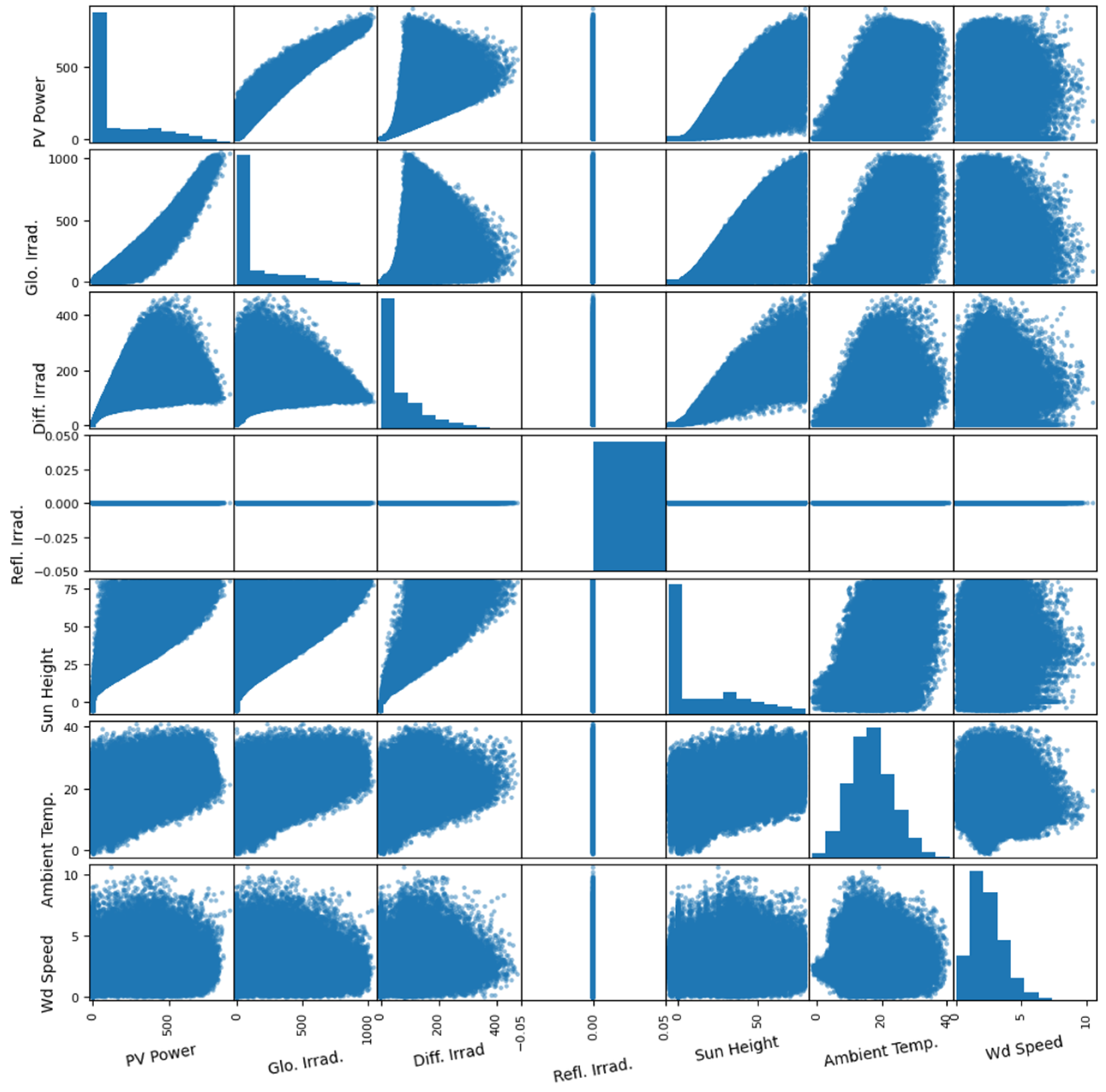
4. Data Description and Variable Selection

4.1. Data Description

We have a time series hourly data having fields for PV output power, normal global irradiance, diffused irradiance, sun height, ambient temperature, reflected irradiance, wind speed, and 24-h time cycle in Grahamstown, Eastern Cape, South Africa for the period from 2009 to 2020. Figure 3 presents the graph of the data—the PV output power.

4.2. Selecting Input Variables

The more variables used as input, the better the performance of the algorithms, but the higher the execution time, the higher the chances of overfitting. To select the variables that will serve as inputs to the algorithms, we consider the interaction between the variables and their correlation with the output power. Figure 4 presents scatterplots of all pairs of attributes. This figure can help one to see the relationship between the variables.

The diagonal plots display the Gaussian distribution of the values of each variable. As expected, there is a strong correlation between global (and diffused) solar irradiance and PV power, but there is no correlation between reflected irradiance and PV power. This fact will be demonstrated more quantitatively later using the Lasso regression analysis. One cannot precisely say for the other variables. We excluded the reflected solar irradiance from the list of input variables.

4.3. Prediction Intervals and Performance Evaluation

4.3.1. Prediction Intervals

The prediction interval (PI) helps energy providers and operators assess the uncertainty level in the electrical energy they supply [50,51]. It is a great tool for measuring uncertainty in model predictions. We will subsequently take a brief look at prediction interval widths.

The prediction interval width (${\mathrm{PIW}}_t$) is the estimated difference between the upper ($U_t$) and lower $L_t$ limits of the values given as follows:

$${\mathrm{PIW}}_t=U_t-L_t t=1, 2, 3, \dots N.$$

(8)

The PI coverage probability (PICP) and PI normalised average width (PINAW) are used to assess the performance of the prediction intervals. The PICP is used to estimate the reliability of the PIs, while PINAW is used to assess the width of the PIs. These two are expressed mathematically as follows [52]:

$$\mathrm{P}\mathrm{I}\mathrm{C}\mathrm{P}=\frac{1}{N}\sum _{t=1}^N{c}_t, {\mathrm{c}}_t=\left\{\begin{array}{c}1 \mathrm{i}\mathrm{f} y_t\in (L_t,U_t)\\ 0 \mathrm{o}\mathrm{t}\mathrm{h}\mathrm{e}\mathrm{r}\mathrm{w}\mathrm{i}\mathrm{s}\mathrm{e}\end{array}\right.,$$

(9)

$$\mathrm{P}\mathrm{I}\mathrm{N}\mathrm{A}\mathrm{W}=\frac{1}{N}\sum _{t=1}^N\frac{{\mathrm{PIW}}_t}{y_{\max }-y_{\min }},$$

(10)

where $y_t$ is the data, and $y_{\min }$ and $y_{\max }$ are the minimum and maximum values of PIW, respectively. The PIs are weighted against a predetermined confidence interval (CI) value. One has valid PI values when the value of PICP is greater than or equal to that predefined CI value. The PI normalised average deviation (PINAD) defines the degree of deviation from the actual value to the PIs and is expressed mathematically as follows [52]:

$$\mathrm{P}\mathrm{I}\mathrm{N}\mathrm{A}\mathrm{D}=\frac{1}{N{(y}_{\max }-y_{\min })}\sum _{t=1}^N{c}_t, {\mathrm{c}}_t=\left\{\begin{array}{l}{L}_t-y_t, \mathrm{i}\mathrm{f} y_t<L_t\\ 0 if L_t\le y_t\le U_t\\ y_t-U_t, \mathrm{i}\mathrm{f} y_t>U_t\end{array}\right..$$

(11)

4.3.2. Performance Matrices

A good number of performance measurement tools are available in the literature. Some are better fit for particular contexts and target objectives.

The mean absolute error (MAE) is the average of the absolute difference between the measured ($y_t$) and predicted (${\widehat{y}}_t$) data. For a total of $N$ predictions, the MAE is given as follows:

$$\mathrm{M}\mathrm{A}\mathrm{E}=\frac{1}{N}\sum _{t=1}^N|y_t-{\widehat{y}}_t|,$$

(12)

The relative MAE (rMAE) gives an MAE value comparable to the measured values. The rMAE is given mathematically as follows:

$$\mathrm{r}\mathrm{M}\mathrm{A}\mathrm{E}=\frac{1}{N}\sum _{t=1}^N\frac{|y_t-{\widehat{y}}_t|}{y_t}.$$

(13)

The root mean squared error (RMSE) is the average of the squared difference between the measured and predicted values. The average of the square of the prediction residual. It is always non-negative and is given as follows:

$$\mathrm{R}\mathrm{M}\mathrm{S}\mathrm{E}=\sqrt{\frac{1}{N}\sum _{t=1}^N{(y_t-{\widehat{y}}_t)}^2}.$$

(14)

The relative RMSE (rRMSE) gives a percentage RMSE value. The rRMSE is given as follows:

$$\mathrm{r}\mathrm{R}\mathrm{M}\mathrm{S}\mathrm{E}=\frac{100}{\overline{y}}\sqrt{\frac{1}{N}\sum _{t=1}^N{(y_t-{\widehat{y}}_t)}^2}.$$

(15)

where $\overline{y}$ is the average of $y_t$, $t=1, 2, 3, \dots N$. The smaller the values for these error metrics, the more accurate the forecasted value.

The R² score is another commonly used metric to measure the performance of a forecast. The R² score can be expressed mathematically as follows:

$${\mathrm{R}}^2=1\frac{{\sum }_{t=1}^N{{(\widehat{y}}_t-y_t)}^2}{{\sum }_{t=1}^N{{(\overline{y}}_t-y_t)}^2},$$

(16)

The closer the value of R² is to 1, the more accurate the prediction of the true value.

It is common practice to normalise (or scale) data before passing through the training step, but we did not practice this in our case because our data had a few missing records and outliers.

4.4. Selecting Input Variables

It is a common practice to use Lasso analysis to perform variable selection, which uses the $\mathcal{l}$ loss function penalty given as follows [5]:

$${\widehat{\mathsf{\beta }}}_{\mathrm{Lasso}}\left(\mathsf{\lambda }\right)=\arg \mathrm{m}\mathrm{i}\mathrm{n}{‖\overrightarrow{y}-\mathsf{{\rm X}}\widehat{\mathsf{\beta }}‖}_2^2+\mathsf{\lambda }{\left|\right|\widehat{\mathsf{\beta }}\left|\right|}_1.$$

(17)

In

Table 2. Parameter coefficient of Lasso regression.

Variables	Coefficients
Global normal irradiance	0.790206
Diffuse irradiance	0.902841
Reflected irradiance	0.000000
Sun elevation	−0.412872
Ambient temperature	−0.817793
Wind speed	1.017501
24-h time cycle	0.186437

, we show the parametric coefficient of the Lasso regression analysis. All the variables except for the reflected irradiance are important forecasting variables.

5. Results

Python Tensor flow and Sklearn (version 1.2.2) are the software packages we used for all our investigations. The implementation details are as follows.

The MLPNN model started with a fully connected layer having 128 neurons and a ReLU activation function, and a final output layer, which consists of a single neuron for output. They complied with MSE as a loss function and Adam optimiser. The compiled model was trained on the training data for 50 epochs.

The CNN model starts with a one-dimensional convolutional layer to extract the features from the input data, then a max pooling layer to reduce the dimensionality of the feature maps (using a pooling size of 8). The data are then flattened and passed through a dense layer with 50 units having a ReLU activation function. Finally, the output layer consists of a single unit used to predict the target value. All these are complied with MSE and Adam as loss function and optimiser, respectively. The compiled model was also trained on the training data for 50 epochs.

The kNN regressor model is initialised with a number of neighbours = 5, algorithm = auto (to allow it to select the best algorithm), leaf size = 30, metric = Minkowski, p = 2 (or L2 norm), and weights = uniform. The initialised model is trained on the training data, and prediction is made on the test data.

Changing hyperparameters of each of the models were performed to see if we can obtain better results but the above configurations produced the best results on our data and are presented below.

5.1. Prediction Results

Figure 5 presents plots of the data and fits of the different models we used in this study for short-term forecasting (38 h ahead) of the solar PV output power for two clear sky days and two cloudy days. The graph in blue is the measured data, while that in red, green, and black are for MLPNN, CNN, and kNN models’ forecasts, respectively. We can see visually from these plots that the prediction produced by kNN best fits the data for these two conditions. MLPNN also produces a reasonably good fit on a clear sky day.

In Figure 6, the density plots of the measured solar PV output power and the different models’ predictions are presented. The solid blue line graph is the measured data, while the dashed lines represent the models’ forecasts. From these graphs, it can be observed that kNN prediction best matches the data, followed closely by the MLPNN predictions. We will subsequently present a qualitative evaluation of these models’ performance.

Figure 6 presents the density plots of the measured solar PV output power together with the models’ predictions during the summer season (top row) on a clear sky day (a) and a cloudy day (b). The same is present for a clear winter sky day (c) and cloudy day (d) on the bottom row. The kNN model’s density graph produced the closest match to the measured data for all four weather conditions under investigation.

Table 3. Evaluating models’ performances on a clear summer sky day (a) and cloudy summer sky day (b) and on clear and cloudy sky days in winter ((c) and (d), respectively).

(a) Clear sky day in summer				(b) Cloudy sky day in summer
	MLPNN	CNN	kNN	MLPNN	CNN	kNN
RMSE	21.42	23.15	4.95	39.35	67.54	2.08
rRMSE	8.69	9.39	2.01	39.40	67.62	2.08
MAE	12.34	14.04	2.74	21.86	46.19	1.11
rMAE	0.49	0.56	0.11	0.91	1.92	0.05
R2	0.99	0.99	1.00	0.92	0.77	1.00
(c) Clear sky day in winter				(d) Cloudy sky day in winter
	MLPNN	CNN	kNN	MLPNN	CNN	kNN
RMSE	10.96	25.69	4.11	17.22	20.09	1.49
rRMSE	9.71	22.77	3.64	32.59	38.04	2.82
MAE	6.47	14.09	2.00	8.18	12.88	0.85
rMAE	0.27	0.59	0.08	0.34	0.54	0.04
R2	1.00	0.98	1.00	0.95	0.93	1.00

presents the results of evaluating our models’ performance using MAE, rMAE, RMSE, rRMSE, and R² metrics for the four weather conditions. The kNN has the overall best performance for these metrics, followed by the MLPNN and then CNN.

5.2. Prediction Accuracy Analysis

This section evaluates how the models’ predictions are centred using PIs and the forecast error distribution.

5.2.1. Prediction Interval Evaluation

In

Table 4. Comparing the performance of the models using PICD, PINAW, and PINAD on a confidence level set to 95% on clear sky and cloudy summer days ((a) and (b), respectively), while the second row presents the same for clear sky and cloudy winter days ((c) and (d) respectively).

(a) Clear sky day in summer				(b) Cloudy sky day in summer
	MLPNN		MLPNN		MLPNN
PICP	28.0	28.95	96	12.5	4.17	91.67
PINAW	0.631	0.622	0.637	0.561	0.633	0.511
PINAD	0.0520	0.0989	0.0002	0.4510	1.0619	0.0011
(c) Clear sky day in winter				(d) Cloudy sky day in winter
	MLPNN		MLPNN		MLPNN
PICP	20.83	20.83	100.0	12.5	4.16	87.50
PINAW	0.507	0.455	0.481	0. 530	0.526	0.495
PINAD	0.0866	0.2212	0.0000	0. 2769	0.5736	0.0016

, we compare the performance confidence intervals of these modes’ predictions using PICP, PINAW, and PINAD with a preset confidence level of 95%. Only the kNN model has a value of PICP greater than 95% on clear sky days. The model with the lowest value for PINAD and the narrowest PINAW is the model that best fits the data [52]. kNN has the smallest PINAD and has the best overall performance with respect to these prediction interval matrices.

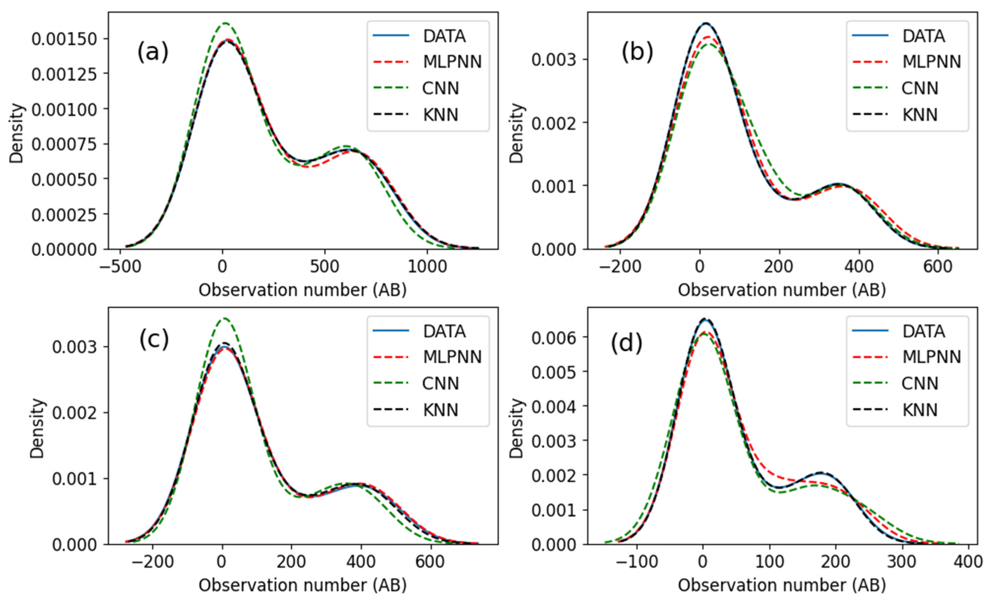
5.2.2. Analysing Residuals

In

Table 5. Comparing residuals of the models’ prediction.

	Median	Min	Max	Mean	Std. Dev.	Skewness	Kurtosis
MLPNN	0.09	−57.31	67.73	−1.36	22.20	0.28	2.56
CNN	0.17	−77.58	30.96	−6.05	24.62	−1.31	1.68
kNN	0.00	−12.54	10.92	1.01	4.39	0.16	1.79

, statistical analyses on the residuals of all the models’ predictions are presented for MLPNN, CNN, and kNN models (with a confidence level of 95%) on a summer clear sky day. The table shows that kNN has the smallest standard deviation among the three models under investigation, which implies that it produces the best fit for the data. MLPNN has the next best fit for the data. kNN and MLPNN have skewness close to zero, meaning their errors have a normal distribution. All the models have a kurtosis value that is less than 3.

Figure 7 presents the whisker and box plots of the residuals of the forecast made with the MLPNN, CNN and kNN models for clear sky and cloudy days during summer and winter seasons. The residual of the kNN model has the smallest tail compared to the others, followed by the forecast made with MLPNN although it made a worst prediction in the summer cloudy day under investigation. It also shows that the kNN model produced the best overall forecast.

5.3. Discussion of Results

This work focused on modelling and forecasting solar PV (hourly) output power for Grahamstown, Eastern Cape, South Africa. We modelled data of PV output power from January 2009 to December 2020. The data were split into 80% training and 20% test data. We modelled the data with MLPNN, CNN, and kNN techniques and used RMSE, rRMSE, MAE, rMAE, and R² performance evaluation matrices to evaluate the models on cloudy and clear days in the summer and winter seasons. The kNN algorithm at its best performance had an RMSE = 1.49%, rRMSE = 2.01%, MAE = 0.85% and rMAE = 0.04%, and RMSE = 4.95%, rRMSE = 3.64%, MAE = 2.74%, and rMAE = 0.11% at its worst performance. The kNN models always had an R² value of 1, while the other methods under investigation had a value of less than 1 in most cases. Also, when a confidence interval analysis on the models with a preset confidence interval of 95% was performed, kNN had a PICP value that was above 95%. All these evaluation matrices show that the kNN algorithm produced the best prediction. One can also draw the same conclusion if you look at whisker and box plots of the residuals of the forecast made by the models under investigation for the four weather conditions, where the kNN model had the smallest tails (compared to that of the other models). The kNN is the best model for our data. Note that the data under investigation have very few spikes (or outliers) and missing records (and are not too noisy), so the kNN model perfectly predicted the data. Again, while MLPNN and CNN each take several minutes to train their respective model, kNN has no training step. It goes straight into modelling the PV output power. So, when it comes to execution time, kNN still wins the contest.

We were inspired by the works of [5,24,53]. Mutavhatsindi et al. [53] analysed the performance of support vector regression, principal component regression, feedforward neural networks, and LSTM networks. Ratshilengo et al. [5] indeed compared the GA algorithm with the RNN and kNN algorithms models’ performance in forecasting global horizontal irradiance. They found the GA algorithm to have the best overall forecast performance. The kNN model in this study produced lower metric values for RMSE, MAE, rRMSE, and rMAE than those produced by [5], although they modelled global solar irradiance while we modelled solar PV output power.

6. Challenges of Photovoltaic Power Forecasting

Forecasting solar PV output power has some challenges. One of these is that it depends on the accuracy of the future weather forecast. Since most PV output power predicting techniques take future weather forecast data as an input parameter, the accuracy of the PV output power prediction is highly dependent on the accuracy of the underlying input weather data [54]. Another challenge is having an enormous amount of data. Even though having large data can help some predicting algorithms to make more accurate predictions, processing large data can consume a lot of machine resources, thereby compromising output speed, especially in cases where real-time data processing is a requirement.

It is often thought that complex models like hybrid and statistical methods will yield more accurate results. Complex models, like most statistical and hybrid models, are often expected to produce more accurate results. This is not always the situation, as simpler methods can produce accurate results if the input vectors are properly preprocessed and filtered. This is also a challenge, as shown by the views held by [55] in selecting the right model and input parameters.

Additionally, the problem of PV solar panel module degradation and site-specific losses exists, which negatively affects medium and long-term forecast horizon estimates. Solar PV output power forecasting models depend on historical data; the forecasted data may defer significantly from the actual PV panels’ output power because of ageing and panel degradation. Hence, although site-specific models have been generated, there is a need to constantly review the model’s input parameters over time based on the degradation of the solar PV modules.

7. Conclusions

This study carried out a performance evaluation of MLPNN, CNN, and kNN methods in modeling solar PV output power for (solar PV installation in) Grahamstown, Eastern Cape, South Africa, for a short-term forecast horizon. Several works are available in literature where the authors modelled solar irradiance with great success. This gives a good indication of the potential electrical energy solar PV systems can provide. This study modelled the actual solar PV output power. It is more beneficial to model the PV output power instead of solar irradiance because it captures the impact of ambient temperature, module temperature, and degradation (as well as other factors) whose rise negatively affects the PV module’s efficiency. After training the models, we analysed their prediction results on sunny and cloudy sky days in summer and winter. The RMSE, rRMSE, MAE, rMAE, and R² performance evaluator are commonly used model evaluation matrices. Applying these performance evaluators to the results of the models under investigation showed that while the CNN model had the worst performance, the kNN model had the overall best performance, followed by the MLPNN model. Statistical analysis performed on the models’ prediction residuals shows that the kNN model had the smallest standard deviation, which implies that it was the best fit for the data. The skewness values of both kNN and MLPNN are close to zero, which indicates a good fit for the data. This study’s findings will be a useful tool for energy providers (both private and public) who want quick and easy but accurate forecasts of their solar photovoltaic installation—to plan energy distribution and expansion of installations in a sustainable and environmentally friendly way.

References

1. Jun, L.; Yuan, Q. The design of distributed photovoltaic charging station for electric vehicles. In Proceedings of the International Conference on Smart Transportation and City Engineering (STCE 2023), 130180H, Chongqing, China, 20–22 October 2023. [Google Scholar]
2. Andrade, J.R.; Bessa, R.J. Improving Renewable Energy Forecasting with a Grid of Numerical Weather Predictions. IEEE Trans. Sustain. Energy 2017, 8, 1571–1580. [Google Scholar] [CrossRef]
3. Sun, S.; Wang, S.; Zhang, G.; Zheng, J. A decomposition-clustering-ensemble learning approach for solar radiation forecasting. Sol. Energy 2018, 163, 189–199. [Google Scholar] [CrossRef]
4. Yang, X.; Jiang, F.; Liu, H. Short-term solar radiation prediction based on SVM with similar data. In Proceedings of the 2nd IET Renewable Power Generation Conference (RPG 2013), Beijing, China, 9–11 September 2013; pp. 1–4. [Google Scholar]
5. Ratshilengo, M.; Sigauke, C.; Bere, A. Short-Term Solar Power Forecasting Using Genetic Algorithms: An Application Using South African Data. Appl. Sci. 2021, 11, 4214. [Google Scholar] [CrossRef]
6. Iheanetu, K.J. Solar Photovoltaic Power Forecasting: A Review. Sustainability 2022, 14, 17005. [Google Scholar] [CrossRef]
7. Das, U.K.; Tey, K.S.; Seyedmahmoudian, M.; Mekhilef, S.; Idris, M.Y.I.; Van Deventer, W.; Horan, B.; Stojcevski, A. Forecasting of photovoltaic power generation and model optimization: A review. Renew. Sustain. Energy Rev. 2018, 81, 912–928. [Google Scholar] [CrossRef]
8. Blanc, P.; Remund, J.; Vallance, L. Short-term solar power forecasting based on satellite images. In Renewable Energy Forecasting: From Models to Applications; Woodhead Publishing: Sawston, UK, 2017; pp. 179–198. [Google Scholar]
9. Wang, G.; Su, Y.; Shu, L. One-day-ahead daily power forecasting of photovoltaic systems based on partial functional linear regression models. Renew. Energy 2016, 96, 469–478. [Google Scholar] [CrossRef]
10. Coimbra, C.F.; Kleissl, J.; Marquez, R. Overview of Solar-Forecasting Methods and A Metric for Accuracy Evaluation; Academic Press: Boston, MA, USA, 2013; pp. 171–194. [Google Scholar]
11. Gensler, A.; Henze, J.; Sick, B.; Raabe, N. Deep Learning for solar power forecasting—An approach using AutoEncoder and LSTM Neural Networks. In Proceedings of the 2016 IEEE International Conference, Systems, Man, and Cybernetics (SMC), Budapest, Hungary, 9 October 2016; pp. 2858–2865. [Google Scholar]
12. Wang, H.; Yi, H.; Peng, J.; Wang, G.; Liu, Y.; Jiang, H.; Liu, W. Deterministic and probabilistic forecasting of photovoltaic power based on deep convolutional neural network. Energy Convers. Manag. 2017, 153, 409–422. [Google Scholar] [CrossRef]
13. Bin, F.; He, J. A short-term photovoltaic power prediction model using cyclical encoding and STL decomposition based on LSTM. In Proceedings of the 2023 3rd International Conference on Electronic Information Engineering and Computer Communication (EIECC), Wuhan, China, 22–24 December 2023; pp. 260–266. [Google Scholar]
14. Saxena, N.; Kumar, R.; Rao, Y.K.S.S.; Mondloe, D.S.; Dhapekar, N.K.; Sharma, A.; Yadav, A.S. Hybrid KNN-SVM machine learning approach for solar power forecasting. Environ. Chall. 2024, 14, 100838. [Google Scholar] [CrossRef]
15. Lima, M.A.F.B.; Carvalho, P.C.M.; Braga, A.P.d.S.; Ramírez, L.M.F.; Leite, J.R. MLP Back Propagation Artificial Neural Network for Solar Resource Forecasting in Equatorial Areas. Renew. Energy Power Qual. J. 2018, 1, 175–180. [Google Scholar] [CrossRef]
16. Costa, R.L.D.C. Convolutional-LSTM networks and generalization in forecasting of household photovoltaic generation. Eng. Appl. Artif. Intell. 2022, 116, 105458. [Google Scholar] [CrossRef]
17. Li, G.; Xie, S.; Wang, B.; Xin, J.; Li, Y.; Du, S. Photovoltaic Power Forecasting with a Hybrid Deep Learning Approach. IEEE Access 2020, 8, 175871–175880. [Google Scholar] [CrossRef]
18. Wang, Y.; Liao, W.; Chang, Y. Gated Recurrent Unit Network-Based Short-Term Photovoltaic Forecasting. Energies 2018, 11, 2163. [Google Scholar] [CrossRef]
19. Gao, B.; Huang, X.; Shi, J.; Tai, Y.; Xiao, R. Predicting day-ahead solar irradiance through gated recurrent unit using weather forecasting data. J. Renew. Sustain. Energy 2019, 11, 043705. [Google Scholar] [CrossRef]
20. Xiang, X.; Li, X.; Zhang, Y.; Hu, J. A short-term forecasting method for photovoltaic power generation based on the TCN-ECANet-GRU hybrid model. Sci. Rep. 2024, 14, 6744. [Google Scholar] [CrossRef] [PubMed]
21. Tajmouati, S.; Wahbi, B.E.L.; Dakkon, M. Applying regression conformal prediction with nearest neighbors to time series data. Commun. Stat.-Simul. Comput. 2024, 53, 1768–1778. [Google Scholar] [CrossRef]
22. Yehor, S.; Kateryna, K. Selection of the K Parameter in the K-Nearest Neighbor Algorithm for Solar Power Prediction. In Proceedings of the 2023 IEEE International Conference on Information and Telecommunication Technologies and Radio Electronics (UkrMiCo), Kyiv, Ukraine, 13–18 November 2023; pp. 306–311. [Google Scholar]
23. Amer, A.Y.A. Global-local least-squares support vector machine (GLocal-LS-SVM). PLoS ONE 2023, 18, e0285131. [Google Scholar]
24. Reyes-Belmonte, M.A. Quo Vadis Solar Energy Research? Appl. Sci. 2021, 11, 3015. [Google Scholar] [CrossRef]
25. Cherkassky, V.; Ma, Y. Practical selection of SVM parameters and noise estimation for SVM regression. Neural Netw. 2004, 17, 113–126. [Google Scholar] [CrossRef] [PubMed]
26. Huang, J.; Korolkiewicz, M.; Agrawal, M.; Boland, J. Forecasting solar radiation on an hourly time scale using a Coupled AutoRegressive and Dynamical System (CARDS) model. Sol. Energy 2013, 87, 136–149. [Google Scholar] [CrossRef]
27. El Hendouzi, A.; Bourouhou, A.; Ansari, O. The Importance of Distance between Photovoltaic Power Stations for Clear Accuracy of Short-Term Photovoltaic Power Forecasting. J. Electr. Comput. Eng. 2020, 2020, 1–14. [Google Scholar] [CrossRef]
28. Luo, X.; Zhang, D.; Zhu, X. Deep learning based forecasting of photovoltaic power generation by incorporating domain knowledge. Energy 2021, 225, 120240. [Google Scholar] [CrossRef]
29. Zhu, H.; Li, X.; Sun, Q.; Nie, L.; Yao, J.; Zhao, G. A Power Prediction Method for Photovoltaic Power Plant Based on Wavelet Decomposition and Artificial Neural Networks. Energies 2015, 9, 11. [Google Scholar] [CrossRef]
30. Xu, Q.; He, D.; Zhang, N.; Kang, C.; Xia, Q.; Bai, J.; Huang, J. A Short-Term Wind Power Forecasting Approach with Adjustment of Numerical Weather Prediction Input by Data Mining. IEEE Trans. Sustain. Energy 2015, 6, 1283–1291. [Google Scholar] [CrossRef]
31. Aminzadeh, F.; De Groot, P. Neural Networks and Other Soft Computing Techniques with Applications in the Oil Industry; Eage Publications: Bunnik, The Netherlands, 2006. [Google Scholar]
32. Hossain, S.; Ong, Z.C.; Ismail, Z.; Noroozi, S.; Khoo, S.Y. Artificial neural networks for vibration based inverse parametric identifications: A review. Appl. Soft Comput. 2017, 52, 203–219. [Google Scholar] [CrossRef]
33. Zhang, Y.; Chen, G.; Malik, O.; Hope, G. An artificial neural network based adaptive power system stabilizer. IEEE Trans. Energy Convers. 1993, 8, 71–77. [Google Scholar] [CrossRef]
34. Moreira, M.O.; Balestrassi, P.P.; Paiva, A.P.; Ribeiro, P.F.; Bonatto, B.D. Design of experiments using artificial neural network ensemble for photovoltaic generation forecasting. Renew. Sustain. Energy Rev. 2021, 135, 110450. [Google Scholar] [CrossRef]
35. Malki, H.A.; Karayiannis, N.B.; Balasubramanian, M. Short-term electric power load forecasting using feedforward neural networks. Expert Syst. 2004, 21, 157–167. [Google Scholar] [CrossRef]
36. Chen, S.M.; Chang, Y.C.; Chen, Z.J.; Chen, C.L. Multiple Fuzzy Rules Interpolation with Weighted Antecedent Variables in Sparse Fuzzy Rule-Based Systems. Int. J. Pattern Recognit. Artif. Intell. 2013, 27, 1359002. [Google Scholar] [CrossRef]
37. Yona, A.; Senjyu, T.; Funabashi, T.; Kim, C.-H. Determination Method of Insolation Prediction with Fuzzy and Applying Neural Network for Long-Term Ahead PV Power Output Correction. IEEE Trans. Sustain. Energy 2013, 4, 527–533. [Google Scholar] [CrossRef]
38. Srisaeng, P.; Baxter, G.S.; Wild, G. An adaptive neuro-fuzzy inference system for forecasting Australia’s domestic low cost carrier passenger demand. Aviation 2015, 19, 150–163. [Google Scholar] [CrossRef]
39. Ali, M.N.; Mahmoud, K.; Lehtonen, M.; Darwish, M.M.F. An Efficient Fuzzy-Logic Based Variable-Step Incremental Conductance MPPT Method for Grid-Connected PV Systems. IEEE Access 2021, 9, 26420–26430. [Google Scholar] [CrossRef]
40. Zhang, J.; Verschae, R.; Nobuhara, S.; Lalonde, J.-F. Deep photovoltaic nowcasting. Sol. Energy 2018, 176, 267–276. [Google Scholar] [CrossRef]
41. Parvez, I.; Sarwat, A.; Debnath, A.; Olowu, T.; Dastgir, M.G.; Riggs, H. Multi-layer Perceptron based Photovoltaic Forecasting for Rooftop PV Applications in Smart Grid. In Proceedings of the 2020 SoutheastCon, Raleigh, NC, USA, 12–15 March 2020; pp. 1–6. [Google Scholar]
42. Hontoria, L.; Aguilera, J.; Zufiria, P. Generation of hourly irradiation synthetic series using the neural network multilayer perceptron. Sol. Energy 2002, 72, 441–446. [Google Scholar] [CrossRef]
43. Pham, B.T.; Tien Bui, D.; Prakash, I.; Dholakia, M.B. Hybrid integration of Multilayer Perceptron Neural Networks and machine learning ensembles for landslide susceptibility assessment at Himalayan area (India) using GIS. CATENA 2017, 149, 52–63. [Google Scholar] [CrossRef]
44. Parvez, I.; Sriyananda, M.G.S.; Güvenç, I.; Bennis, M.; Sarwat, A. CBRS Spectrum Sharing between LTE-U and WiFi: A Multiarmed Bandit Approach. Mob. Inf. Syst. 2016, 2016, 5909801. [Google Scholar] [CrossRef]
45. Suresh, V.; Janik, P.; Rezmer, J.; Leonowicz, Z. Forecasting Solar PV Output Using Convolutional Neural Networks with a Sliding Window Algorithm. Energies 2020, 13, 723. [Google Scholar] [CrossRef]
46. Babalhavaeji, A.; Radmanesh, M.; Jalili, M.; Gonzalez, S. Photovoltaic generation forecasting using convolutional and recurrent neural networks. Energy Rep. 2023, 9, 119–123. [Google Scholar] [CrossRef]
47. Horton; Mukai, Y.; Nakai, K. Protein Subcellular Localization Prediction. Pract. Bioinformatician 2004, 193–216. [Google Scholar] [CrossRef]
48. Liu, Z.; Zhang, Z. Solar forecasting by K-Nearest Neighbors method with weather classification and physical model. In Proceedings of the 2016 North American power symposium (NAPS), Denver, CO, USA, 18–20 September 2016; pp. 1–6. [Google Scholar]
49. Kohavi, R.; John, G.H. Wrappers for feature subset selection. Artif. Intell. 1995, 97, 273–324. [Google Scholar] [CrossRef]
50. Chatfield, C. Calculating Interval Forecasts. J. Bus. Econ. Stat. 1993, 11, 121–135. [Google Scholar] [CrossRef]
51. Gaba, A.; Tsetlin, I.; Winkler, R.L. Combining Interval Forecasts. Decis. Anal. 2017, 14, 1–20. [Google Scholar] [CrossRef]
52. Sun, X.; Wang, Z.; Hu, J. Prediction Interval Construction for Byproduct Gas Flow Forecasting Using Optimized Twin Extreme Learning Machine. Math. Probl. Eng. 2017, 2017, 5120704. [Google Scholar] [CrossRef]
53. Mutavhatsindi, T.; Sigauke, C.; Mbuvha, R. Forecasting Hourly Global Horizontal Solar Irradiance in South Africa Using Machine Learning Models. IEEE Access 2020, 8, 198872–198885. [Google Scholar] [CrossRef]
54. Sengupta, M.; Habte, A.; Wilbert, S.; Gueymard, C.; Remund, J. Best Practices Handbook for the Collection and Use of Solar Resource Data for Solar Energy Applications, 3rd ed.; National Renewable Energy Laboratory (NREL): Golden, CO, USA, 2021.
55. Dolara, A.; Grimaccia, F.; Leva, S.; Mussetta, M.; Ogliari, E. A Physical Hybrid Artificial Neural Network for Short Term Forecasting of PV Plant Power Output. Energies 2015, 8, 1138–1153. [Google Scholar] [CrossRef]
Figure 1. (a) Schematic representation of a typical ANN having the input, hidden, and output layers. (b) A pictorial presentation of a mathematical model of an ANN cell [6].
Optics 05 00021 g001
Figure 2. Schematic representation of a convolutional network.
Optics 05 00021 g002
Figure 3. Plot the PV output power from 2009 to 2020.
Optics 05 00021 g003
Figure 4. Plots of the variables.
Optics 05 00021 g004
Figure 5. Plots of the solar PV output power data together with the graphs of MLPNN, CNN, and kNN models’ predictions (dash lines) on a clear summer sky day (a) and cloudy day (b). The same plots are shown for a clear winter sky day (c) and a cloudy day (d). The solid lines represent the measured data, while the dashed line represents the predictions.
Optics 05 00021 g005
Figure 6. Density plots of the measured data (solid line) together with each model’s forecast (dash lines). In the top row is the graph for the models’ predictions on a clear summer sky day (a) and cloudy day (b), while the bottom panel presents the same on a clear winter sky day (c) and cloudy day (d).
Optics 05 00021 g006
Figure 7. Whisker and box plots of the residuals of the forecast made with MLPNN, CNN, and kNN models on clear sky (a) and cloudy sky (b) days during the summer season and on clear sky (c) and cloudy sky (d) days during the winter season.
Optics 05 00021 g007