Theoretical Advancements on a Few New Dependence Models Based on Copulas with an Original Ratio Form

Abstract

Copulas are well-known tools for describing the relationship between two or more quantitative variables. They have recently received a lot of attention, owing to the variable dependence complexity that appears in heterogeneous modern problems. In this paper, we offer five new copulas based on a common original ratio form. All of them are defined with a single tuning parameter, and all reduce to the independence copula when this parameter is equal to zero. Wide admissible domains for this parameter are established, and the mathematical developments primarily rely on non-trivial limits, two-dimensional differentiations, suitable factorizations, and mathematical inequalities. The corresponding functions and characteristics of the proposed copulas are looked at in some important details. In particular, as common features, it is shown that they are diagonally symmetric, but not Archimedean, not radially symmetric, and without tail dependence. The theory is illustrated with numerical tables and graphics. A final part discusses the multi-dimensional variation of our original ratio form. The contributions are primarily theoretical, but they provide the framework for cutting-edge dependence models that have potential applications across a wide range of fields. Some established two-dimensional inequalities may be of interest beyond the purposes of this paper.

1. Introduction

In data analysis, modeling the association (or dependence) between two or more variables is crucial. To capture and quantify such associations, a number of ideas have been put forth in the literature. When quantitative variables are considered, the idea of copulas continues to be one of the most helpful among them. A copula can be thought of as a cutting-edge tool for modeling and expressing various relationships among continuous random variables, giving additional freedom for creating multivariate stochastic models. The applications are in a variety of applied fields, including informatics, engineering, insurance, physics, hydrology, medicine, astronomy, etc. See [1,2,3,4], among others. If we restrict our attention to the two-dimensional case, a copula is defined as a cumulative distribution function on ${[0,1]}^2$, with continuous uniform marginal distributions. A precise definition of a two-dimensional copula in the absolutely continuous case is proposed below (see [5]).

Definition 1.

The function C: [0,1]${}^2\to$ [0,1] is an (absolutely continuous) two-dimensional copula if and only if

(i) we have $C(x,0)=C(0,y)=0$ for any $(x,y)\in {[0,1]}^2$,

(ii) we have $C(x,1)=x$ and $C(1,y)=y$ for any $(x,y)\in {[0,1]}^2$,

(iii) we have (in the absolutely continuous case)

$${\displaystyle {\partial }_{x,y}C(x,y)\ge 0}$$

for any $(x,y)\in {[0,1]}^2$, where ${\partial }_{x,y}={\partial }^2/(\partial x\partial y)$ denotes the mixed second order partial derivatives according to x and y.

Theory, examples, inferences, and applications can be found in the following avoidable references: [5,6,7,8,9]. The commonly used copulas include the Ali–Mikhail–Haq, Clayton, Farlie–Gumbel–Morgenstern (FGM), Frank, Fréchet, Gumbel–Barnett (GB), Hüsler–Reiss, Joe, Marshall–Olkin, and Plackett copulas. With the computational developments and extensive data analysis, the existing copulas have shown some limits, and the need for more original copulas has arisen. As a result, many authors have devised novel strategies for producing copulas with unique forms and manageable dependence properties. See [10,11,12,13,14,15,16,17,18,19,20,21], among others. In particular, the contemporary works of [14,17] have attracted our attention.

• In [17], copulas of the following product form are investigated:

  $$\begin{array}{c}\hfill C(x,y)=xy\varphi \left[(1-x)(1-y)\right],(x,y)\in {[0,1]}^2,\end{array}$$

  (1)

  where $\varphi \left(x\right)$ is a uni-dimensional function that has certain properties (which will be omitted here). The construction of the FGM copula has clearly inspired this form. By tuning the function $\varphi \left(x\right)$, the resulting copulas innovate by proposing entirely new dependence models based on various functional natures. In [17], many examples are offered.
• One may also mention the original approach in [14], generating copulas of the following polyno-exponential form:

  $$\begin{array}{c}\hfill C(x,y)=xyexp\left[-\varphi \left(x\right)\psi \left(y\right)\right],(x,y)\in {[0,1]}^2,\end{array}$$

  (2)

  where $\varphi \left(x\right)$ and $\psi \left(x\right)$ are two distinct uni-dimensional functions that satisfy certain properties (which we will ignore here). It is obvious that this form was influenced by the way the GB copula is constructed. Copulas of this kind are innovative in that they present completely novel dependence models, frequently with a substantial negative dependence and based on different functional natures. Numerous examples are given in [14].

Two simple examples of the copulas in Equations (1) and (2) are the independence copula, i.e., $\mathsf{\Pi }(x,y)=xy$, and the Celebioglu–Cuadras (CC) copula defined by

$$C_{\alpha }(x,y)=xyexp\left[\alpha (1-x)(1-y)\right],(x,y)\in {[0,1]}^2,$$

with $\alpha \in [-1,1]$. The CC copula is recognized to be particularly adaptable in terms of dependent qualities and has a straightforward mathematical structure. We refer to [22,23,24] for more information.

The functional generalization schemes in Equations (1) and (2), combined with the rarity of non-Archimedean ratio copulas in the literature, lead to a novel insight when considering copulas of the following form:

$$\begin{array}{c}\hfill C(x,y)=xy\frac{\varphi \left(x\right)\varphi \left(y\right)}{\varphi \left(1\right)\varphi \left(xy\right)},(x,y)\in {[0,1]}^2,\end{array}$$

(3)

where $\varphi \left(x\right)$ is a specific uni-dimensional function. As a result, $C(x,y)$ can be viewed as a multiplicatively perturbed version of the independence copula $\mathsf{\Pi }(x,y)$. Because of the term $\varphi \left(xy\right)$ in the denominator, the perturbed function can be non-separable with respect to x and y, which is a quite unusual form in a copula setting. Indeed, there are only a few known examples of this type of copula, including the independence copula and the CC copula derived from the function $\varphi \left(x\right)=exp(-\alpha x)$. One can also mention the new ratio (NR) copula introduced in [25] and obtained with $\varphi \left(x\right)=2-x$. The lack of other referenced examples, as well as the originality of the form in Equation (3), are motivations for further research in this area. As a result, this paper does it by examining such copulas. Instead of conducting a global study, which may imply unnecessary conditions (especially on the parameter ranges), we will concentrate on a few specific cases. More specifically, five two-dimensional copulas are introduced, each based on one of five types of functions $\varphi \left(x\right)$ (ratio-polynomial, polynomial, sine, arctangent, and so on). They all depend on only one tuning parameter. To the best of our knowledge, the resulting ratio copulas are new in the literature. For each function, we determine the admissible values of the parameter. The proofs are not trivial; they are mainly based on limit, two-dimensional differentiation, factorization, and mathematical inequalities. Subsequently, we examine the main properties of the proposed copulas, such as their shapes, related functions, symmetry, expansions (when available), tail dependences, medial and Spearman correlations, and two-dimensional distribution generation. It is demonstrated that they are diagonally symmetric, but not Archimedean, not radially symmetric, and not tail dependent, as common characteristics. When appropriate, numerical and graphical analyses are provided. Then, based on Equation (3), a natural multi-dimensional version of the ratio copula form is discussed. In particular, a multi-dimensional version of the first introduced is established, and it reveals itself to be particularly simple and manageable. This can be viewed as a first step toward the construction of new multi-dimensional ratio copulas, which remain of particular interest in some applied fields. Several two-dimensional inequalities, on the other hand, are discovered and might be of independent interest.

The rest of the paper is composed of the following sections: Section 2 presents the first ratio copula based on a ratio-polynomial function, along with its properties. Section 3, Section 4, Section 5 and Section 6 are analogous to Section 2, but for the four other ratio-type copulas, based on polynomial, sine, arctangent, and logarithmic functions, respectively. Section 7 emphasizes an appropriate multi-dimensional setting. A summary of the findings is proposed in Section 8.

2. Ratio-Polynomial Copula

2.1. Presentation

The result below considers the copula form in Equation (3), with $\varphi \left(x\right)=1/(1+\alpha x)$, where $\alpha$ denotes a tuning parameter.

Proposition 1.

The following two-dimensional function represents a valid copula:

$$\begin{array}{c}\hfill C_{\alpha }(x,y)=xy\frac{(1+\alpha )(1+\alpha xy)}{(1+\alpha x)(1+\alpha y)},(x,y)\in {[0,1]}^2,\end{array}$$

(4)

for $\alpha \ge -1/4$.

Proof. 

The proof is based on Definition 1, and limit, differentiation, well-chosen factorization techniques, and polynomial inequalities.

(i) For any $x\in [0,1]$, we have

$$C_{\alpha }(x,0)=x\times 0\times \frac{(1+\alpha )(1+\alpha x\times 0)}{(1+\alpha x)(1+\alpha \times 0)}=0.$$

Using a similar development, for any $y\in [0,1]$, we obtain $C_{\alpha }(0,y)=0$.

(ii) For any $x\in [0,1]$, we have

$$C_{\alpha }(x,1)=x\times 1\times \frac{(1+\alpha )(1+\alpha x\times 1)}{(1+\alpha x)(1+\alpha \times 1)}=x.$$

Similarly, for any $y\in [0,1]$, we have $C_{\alpha }(1,y)=y$.

(iii) Using standard differentiation techniques and appropriate factorizations (hereafter, “appropriate” means “to choose a manageable one after a lot of possibilities tested”), for any $(x,y)\in {[0,1]}^2$, we have

$$\begin{array}{cc}\hfill & {\partial }_{x,y}{C}_{\alpha }(x,y)=(1+\alpha )\frac{1+\alpha xy(2+\alpha x)(2+\alpha y)}{{(1+\alpha x)}^2{(1+\alpha y)}^2}.\hfill \end{array}$$

It is clear that, for $\alpha \ge -1/4$ and any $(x,y)\in {[0,1]}^2$, we have $1+\alpha >0$, ${(1+\alpha x)}^2>0$, and ${(1+\alpha y)}^2>0$. For $\alpha \ge 0$, it is immediate that $1+\alpha xy(2+\alpha x)(2+\alpha y)\ge 0$. On the other hand, for $\alpha \in [-1/4,0)$, since $2+\alpha x\in (0,2]$ and $2+\alpha y\in (0,2]$, we have

$$1+\alpha xy(2+\alpha x)(2+\alpha y)\ge 1+4\alpha xy\ge 1+4\alpha \ge 0.$$

Hence, for $\alpha \ge -1/4$, we have

$${\partial }_{x,y}{C}_{\alpha }(x,y)\ge 0.$$

The point (iii) is proved.

The proof of the proposition ends. □

Remark 1.

If the function $\varphi \left(x\right)=\gamma x^{\beta }/(1+\alpha x)$ is considered in Equation (3), where β and γ are tuning parameters, Proposition 1 holds; the definition of the copula in Equation (4) is unchanged because the term $\gamma x^{\beta }$ vanished immediately with the ratio transformation.

For the purpose of this paper, the copula defined in Equation (4) is called the ratio-polynomial (RP) copula. Plots of the RP copula are presented in Figure 1 and Figure 2, for $\alpha =-1/4$ and $\alpha =1$ (arbitrarily chosen in the admissible domain), respectively.

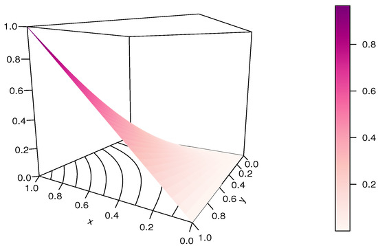
Figure 1. Plots of the shapes and contours of the RP copula for $\alpha =-1/4$.

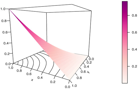
Figure 2. Plots of the shapes and contours of the RP copula for $\alpha =1$.

From these figures, different shape morphologies are observed for the RP copula. The impact of $\alpha$ on them is certain.

2.2. Related Functions and Copulas

This section is devoted to some interesting functions related to the RP copula.

2.2.1. Main Functions

To begin, based on Equation (4), the RP copula density is calculated as

$$\begin{array}{c}\hfill c_{\alpha }(x,y)={\partial }_{x,y}{C}_{\alpha }(x,y)=(1+\alpha )\frac{1+\alpha xy(2+\alpha x)(2+\alpha y)}{{(1+\alpha x)}^2{(1+\alpha y)}^2},(x,y)\in {[0,1]}^2.\end{array}$$

The shapes of this function are of particular interest to see: (i) the modeling possibilities of the RP copula, and (ii) the influence of the parameter $\alpha$ on these shapes. Plots of the RP copula density are presented in Figure 3 and Figure 4, again for $\alpha =-1/4$ and $\alpha =1$, respectively.

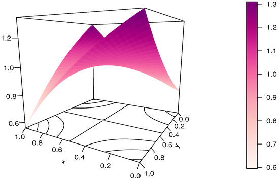
Figure 3. Plots of the shapes and contours of the RP copula density for $\alpha =-1/4$.

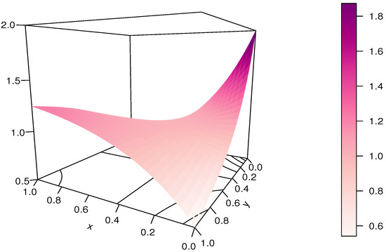
Figure 4. Plots of the shapes and contours of the RP copula density for $\alpha =1$.

The shapes of the RP copula density are completely different in these figures, illustrating a kind of dependence flexibility. Again, the impact of $\alpha$ on these shapes is crucial, and on the extreme points $(0,0)$, $(1,1)$, $(0,1)$ and $(1,0)$ in particular. Further results on this subject will be proved theoretically.

The RP survival copula is obtained as

$$\begin{array}{cc}\hfill & {\widehat{C}}_{\alpha }(x,y)=x+y-1+C_{\alpha }(1-x,1-y)\hfill \\ \hfill & =x+y-1+(1-x)(1-y)\frac{(1+\alpha )\left[1+\alpha (1-x)(1-y)\right]}{\left[1+\alpha (1-x)\right]\left[1+\alpha (1-y)\right]},(x,y)\in {[0,1]}^2.\hfill \end{array}$$

It is also a new copula to add in the existing literature, under the assumption that $\alpha \ge -1/4$.

Several other related copulas can be considered based on $C_{\alpha }(x,y)$, such as the x-flipping copula defined by ${\tilde{C}}_{\alpha }(x,y)=y-C_{\alpha }(1-x,y)$ or the y-flipping copula defined by ${\overline{C}}_{\alpha }(x,y)=x-C_{\alpha }(x,1-y)$ (see [5]). We omit their expressions for the sake of space.

2.2.2. Product of Copulas

The copula product of two two-dimensional copulas, say $C^{\left(1\right)}(x,y)$ and $C^{\left(2\right)}(x,y)$, is defined by

$$(C^{\left(1\right)}★C^{\left(2\right)})(x,y)={\int }_0^1\left[{\partial }_y{C}^{\left(1\right)}(x,t)\right]\left[{\partial }_x{C}^{\left(2\right)}(t,y)\right]dt,(x,y)\in {[0,1]}^2,$$

where ${\partial }_y$ denotes the first order partial derivative with respect to y, and the same when we substitute y by x. The main interest of this product is that $(C^{\left(1\right)}★C^{\left(2\right)})(x,y)$ is a valid copula, opening the door to various forms based on diverse combinations of $C^{\left(1\right)}(x,y)$ and $C^{\left(2\right)}(x,y)$. We refer to [26], and the references therein. Here, some closed-form expressions are demonstrated by taking $C^{\left(1\right)}(x,y)=C_{\alpha }(x,y)$.

To begin, we define the RP product copula by the copula product of the RP copula with itself, that is $C_{\alpha }^{\times }(x,y)=(C_{\alpha }★C_{\alpha })(x,y)$. One interest is that it has a closed-form expression, which is an unusual quality for a ratio copula, as shown in the following result.

Lemma 1.

The RP product copula has the following expression:

$$C_{\alpha }^{\times }(x,y)=xy\left(1+{\tau }_{\alpha }\frac{(1-x)(1-y)}{(1+\alpha x)(1+\alpha y)}\right),(x,y)\in {[0,1]}^2,$$

where

$${\tau }_{\alpha }=\frac{{\alpha }^2}{3(1+\alpha )},$$

with $\alpha \ge -1/4$.

Proof. 

After differentiation, substitution, and integration, we have

$$\begin{array}{cc}\hfill C_{\alpha }^{\times }(x,y)& =(C_{\alpha }★C_{\alpha })(x,y)={\int }_0^1\left[{\partial }_y{C}_{\alpha }(x,t)\right]\left[{\partial }_x{C}_{\alpha }(t,y)\right]dt\hfill \\ \hfill & ={\int }_0^1(1+\alpha )x\frac{1+2\alpha xt+{\alpha }^{2}x{t}^2}{(1+\alpha x){(1+\alpha t)}^2}\times (1+\alpha )y\frac{1+2\alpha ty+{\alpha }^2{t}^{2}y}{(1+\alpha y){(1+\alpha t)}^2}dt\hfill \\ \hfill & ={(1+\alpha )}^2\frac{xy}{(1+\alpha x)(1+\alpha y)}{\int }_0^1\frac{1}{{(1+\alpha t)}^4}(1+2\alpha xt+{\alpha }^{2}x{t}^2)(1+2\alpha ty+{\alpha }^2{t}^{2}y)dt\hfill \\ \hfill & ={(1+\alpha )}^2\frac{xy}{(1+\alpha x)(1+\alpha y)}\frac{\alpha \left\{y\right[(3\alpha +4)\alpha x+2\alpha +3]+2\alpha x+\alpha +3x+3\}+3}{3{(1+\alpha )}^3}\hfill \\ \hfill & =xy\frac{3{\alpha }^{3}xy+3\alpha (x+y+1)+{\alpha }^2(2x+1)(2y+1)+3}{3(1+\alpha )(1+\alpha x)(1+\alpha y)}\hfill \\ \hfill & =xy\left(1+{\tau }_{\alpha }\frac{(1-x)(1-y)}{(1+\alpha x)(1+\alpha y)}\right).\hfill \end{array}$$

This ends the proof of Lemma 1. □

It is worth noting that, for $\alpha \ge -1/4$, we have ${\tau }_{\alpha }\ge 0$. Let us now recall that the FGM copula can be defined by

$$C_{\theta }^{†}(x,y)=xy\left[1+\theta (1-x)(1-y)\right],(x,y)\in {[0,1]}^2,$$

with $\theta \in [-1,1]$ (see [16]). Thus, the RP and FGM copulas have functional similarities with a ratio-polynomial term as their main difference. In this sense, the RP copula is a modified version of the FGM copula, but it does not include it as a special case because ${lim}_{\alpha \to 0}{\tau }_{\alpha }=0$. To our knowledge, this ratio-type modification is completely novel in the literature.

We now present another result mixing the RP and FGM copula. We define the RP-FGM product copula by $C_{\alpha ,\theta }^{\times }(x,y)=(C_{\alpha }★C_{\theta }^{†})(x,y)$. The next result demonstrates that it has an interesting closed form expression.

Lemma 2.

The RP-FGM product copula has the following expression:

$$C_{\alpha ,\theta }^{\times }(x,y)=xy\left(1+{\upsilon }_{\alpha ,\theta }\frac{(1-x)(1-y)}{1+\alpha x}\right),(x,y)\in {[0,1]}^2,$$

where

$${\upsilon }_{\alpha ,\theta }=\theta \frac{\alpha (\alpha +2)-2(1+\alpha )log(1+\alpha )}{{\alpha }^2},$$

with $\alpha \ge -1/4$ and $\theta \in [-1,1]$.

Proof. 

After differentiation, substitution, and integration, we have

$$\begin{array}{cc}\hfill C_{\alpha ,\theta }^{\times }(x,y)& =(C_{\alpha }★C_{\theta }^{†})(x,y)={\int }_0^1\left[{\partial }_y{C}_{\alpha }(x,t)\right]\left[{\partial }_x{C}_{\theta }^{†}(t,y)\right]dt\hfill \\ \hfill & ={\int }_0^1(1+\alpha )x\frac{1+2\alpha xt+{\alpha }^{2}x{t}^2}{(1+\alpha x){(1+\alpha t)}^2}\times y\left[1+\theta (1-2t)(1-y)\right]dt\hfill \\ \hfill & =(1+\alpha )\frac{xy}{1+\alpha x}{\int }_0^1\frac{1+2\alpha xt+{\alpha }^{2}x{t}^2}{{(1+\alpha t)}^2}\left[1+\theta (1-2t)(1-y)\right]dt\hfill \\ \hfill & =(1+\alpha )\frac{xy}{1+\alpha x}\frac{\alpha \left[\alpha +{\alpha }^{2}x+\theta (\alpha +2)(1-x)(1-y)\right]-2\theta (\alpha +1)(1-x)(1-y)log(1+\alpha )}{{\alpha }^2(1+\alpha )}\hfill \\ \hfill & =xy\left(1+{\upsilon }_{\alpha ,\theta }\frac{(1-x)(1-y)}{1+\alpha x}\right).\hfill \end{array}$$

Lemma 2 is proved. □

It should be noted that the RP-FGM product copula is not diagonally symmetric, and ${\upsilon }_{\alpha ,\theta }\in [-1,1]$. It can be viewed as an extension of the FGM copula thanks to the presence of $\alpha$, but it does not cover it as a special case since ${lim}_{\alpha \to 0}{\upsilon }_{\alpha ,\theta }=0$.

Due to the non-diagonal symmetry, the following copula is immediately derived from the RP-FGM product copula:

$$C_{\alpha ,\theta }^{{\times }^{\prime }}(x,y)=xy\left(1+{\upsilon }_{\alpha ,\theta }\frac{(1-x)(1-y)}{1+\alpha y}\right),(x,y)\in {[0,1]}^2,$$

with $\alpha \ge -1/4$ and $\theta \in [-1,1]$, and it corresponds to the FGM-RP product copula.

Other copula products based on the RP copula have been investigated, but few of them present a manageable expression.

2.3. Properties

Some key characteristics of the RP copula are now discussed. All the coming notions can be found in the book of [5]. Clearly, the RP copula is diagonally symmetric because $C_{\alpha }(x,y)=C_{\alpha }(y,x)$ for any $(x,y)\in {[0,1]}^2$. It is not Archimedean, because, for $\alpha =1$ (for instance), it is not associative. Indeed, we have

$$\begin{array}{c}\hfill C_{\alpha }\left[\frac{1}{4},C_{\alpha }\left(\frac{1}{2},\frac{1}{3}\right)\right]=0.06828165\ne 0.06847826=C_{\alpha }\left[C_{\alpha }\left(\frac{1}{4},\frac{1}{2}\right),\frac{1}{3}\right].\end{array}$$

The RP copula is not radially symmetric because there exists $(x,y)$ such that ${\widehat{C}}_{\alpha }(x,y)\ne C_{\alpha }(x,y)$.

The following result is about the quadrant dependence of the RP copula.

Lemma 3.

For $\alpha \in [-1/4,0)$, the RP copula is negatively quadrant dependent, i.e., $C_{\alpha }(x,y)\le xy$ for any $(x,y)\in {[0,1]}^2$. For $\alpha \in (0,1]$, it is positively quadrant dependent, i.e., $C_{\alpha }(x,y)\ge xy$ for any $(x,y)\in {[0,1]}^2$.

Proof. 

Let us remark that

$${\partial }_{\alpha }{C}_{\alpha }(x,y)=xy(1-x)(1-y)\frac{1-{\alpha }^{2}xy}{{(1+\alpha x)}^2{(1+\alpha y)}^2}.$$

For $\alpha \in [-1/4,1]$ and any $(x,y)\in {[0,1]}^2$, we have $1-{\alpha }^{2}xy\ge 0$, implying that ${\partial }_{\alpha }{C}_{\alpha }(x,y)\ge 0$. Therefore, $C_{\alpha }(x,y)$ is an increasing function with respect to $\alpha$ for $\alpha \in [-1/4,1]$. Then, for $\alpha \in [-1/4,0)$ and any $(x,y)\in {[0,1]}^2$, we have $C_{\alpha }(x,y)\le C_0(x,y)=xy$, and, for $\alpha \in (0,1]$, we have $C_{\alpha }(x,y)\ge C_0(x,y)=xy$. This ends the proof of Lemma 3. □

Some other properties of the RP copula are listed below.

Of course, as for any copula, the Fréchet–Hoeffding bounds hold: For any $(x,y)\in {[0,1]}^2$, we have $max(x+y-1,0)\le C_{\alpha }(x,y)\le min(x,y)$.

Remark 2.

As a consequence of the Fréchet–Hoeffding bounds, the following inequalities are derived, which can be of independent interest: For $\alpha \ge -1/4$ and any $(x,y)\in {[0,1]}^2$, we have

$$max(x+y-1,0)(1+\alpha x)(1+\alpha y)\le (1+\alpha )xy(1+\alpha xy)\le min(x,y)(1+\alpha x)(1+\alpha y).$$

Several new two-dimensional inequalities can be derived. For example, if we only consider the right inequality, we can deduce $(1+\alpha )xy(1+\alpha xy)\le x(1+\alpha x)(1+\alpha y)$ and $(1+\alpha )xy(1+\alpha xy)\le y(1+\alpha x)(1+\alpha y)$. Additionally, by writing $min(x,y)=(x+y-|x-y\left|\right)/2$, the following inequality holds:

$$|x-y|(1+\alpha x)(1+\alpha y)+2(1+\alpha )xy(1+\alpha xy)\le (x+y)(1+\alpha x)(1+\alpha y).$$

Taking $x=y$ as another example with a smaller dimension, we obtain $(1+\alpha )x^2(1+\alpha x^2)\le x{(1+\alpha x)}^2$. All these inequalities can be used in various mathematical contexts (analysis, physics, etc.).

For $\alpha \in [-1/4,1)$ and any $(x,y)\in {[0,1)}^2$, by using the geometric series formula, we obtain the following power decomposition:

$$C_{\alpha }(x,y)=\sum _{i=0}^{\infty }\sum _{j=0}^{\infty }{\gamma }_{i,j}(1+\alpha xy)x^{i+1}{y}^{j+1},$$

where ${\gamma }_{i,j}=(1+\alpha ){(-1)}^{i+j}{\alpha }^{i+j}$. The RP copula density follows as

$$c_{\alpha }(x,y)=\sum _{i=0}^{\infty }\sum _{j=0}^{\infty }{\gamma }_{i,j}\left[(i+1)(j+1)x^i{y}^j+\alpha (i+2)(j+2)x^{i+1}{y}^{j+1}\right].$$

From this expansion, we can provide an expansion of the related $(r,s)$-th moment defined by

$${\mu }_{r,s}=\sum _{i=0}^{\infty }\sum _{j=0}^{\infty }{\gamma }_{i,j}\left[\frac{(i+1)(j+1)}{(i+r+1)(j+s+1)}+\alpha \frac{(i+2)(j+2)}{(i+r+2)(j+s+2)}\right].$$

Let us now investigate the possible tail dependence of the RP copula. Using standard limit techniques, we have

$${\lambda }_L=\underset{x\to 0}{lim}\frac{C_{\alpha }(x,x)}{x}=\underset{x\to 0}{lim}x\frac{(1+\alpha )(1+\alpha x^2)}{{(1+\alpha x)}^2}=0$$

and

$${\lambda }_U=\underset{x\to 1}{lim}\frac{1-2x+C_{\alpha }(x,x)}{1-x}=\underset{x\to 1}{lim}\frac{1-2x+x^2(1+\alpha )(1+\alpha x^2)/{(1+\alpha x)}^2}{1-x}=0.$$

It is concluded that the RP copula has no tail dependence.

The medial correlation of the RP copula is simply indicated as

$$M=4C_{\alpha }\left(\frac{1}{2},\frac{1}{2}\right)-1=\frac{(1+\alpha )(4+\alpha )}{{(2+\alpha )}^2}-1.$$

The rho of Spearman of the RP copula is defined by

$$\rho =12{\int }_0^1{\int }_0^1{C}_{\alpha }(x,y)dxdy-3.$$

As an advantage of the RP copula, this measure has a closed form, as presented in the lemma below.

Lemma 4.

The rho of Spearman of the RP copula can be expressed as

$$\rho =\frac{3}{{\alpha }^5}{\left[\alpha (\alpha +2)-2(1+\alpha )log(1+\alpha )\right]}^2,$$

for $\alpha \ge -1/4$.

Proof. 

By several integrations, we obtain

$$\begin{array}{cc}\hfill & {\int }_0^1{\int }_0^1{C}_{\alpha }(x,y)dxdy={\int }_0^1\left[{\int }_0^{1}xy\frac{(1+\alpha )(1+\alpha xy)}{(1+\alpha x)(1+\alpha y)}dx\right]dy\hfill \\ \hfill & =\frac{1+\alpha }{2{\alpha }^2}{\int }_0^{1}y\frac{\alpha (2+(\alpha -2\left)y\right)-2(1-y)log(1+\alpha )}{1+\alpha y}dy\hfill \\ \hfill & =\frac{1+\alpha }{4{\alpha }^5}\left[({\alpha }^2+4){\alpha }^2+4(\alpha +1){log}^2(1+\alpha )-4(\alpha +2)\alpha log(1+\alpha )\right].\hfill \end{array}$$

Hence,

$$\begin{array}{cc}\hfill \rho & =3\left(\frac{1+\alpha }{{\alpha }^5}\left[({\alpha }^2+4){\alpha }^2+4(\alpha +1){log}^2(1+\alpha )-4(\alpha +2)\alpha log(1+\alpha )\right]-1\right)\hfill \\ \hfill & =\frac{3}{{\alpha }^5}{\left[\alpha (\alpha +2)-2(1+\alpha )log(1+\alpha )\right]}^2.\hfill \end{array}$$

This ends the proof of Lemma 4. □

Based on Lemma 4, it is clear that $\rho >0$ for $\alpha >0$, and $\rho <0$ for $\alpha <0$. Additionally, for $\alpha \ge -1/4$, we have $\rho \le 3/\alpha$, with $\rho \sim 3/\alpha$ when $\alpha \to 0$ and $\rho \sim 3/\alpha$ when $\alpha \to \infty$. It can also be shown that ${sup}_{\alpha \in [-1/4,\infty )}\rho \approx 0.18922$ at $\alpha \approx 2.6746$. Since, at $\alpha =-1/4$, we have $\rho \approx -0.1097418$, we conclude that

$$\rho \in [-0.11,0.19],$$

which corresponds to a moderate dependence.

Other measures of association with clear analytical expressions are collected in Table 1.

Table 1. Other measures of association with the RP copula.

Name	Formula	Value
Gini gamma	${\displaystyle 4{\int }_0^1\left[C_{\alpha }(x,x)+C_{\alpha }(x,1-x)\right]dx-2}$	${\displaystyle \frac{2({\alpha }^2+6\alpha +6)}{{\alpha }^3}-\frac{8(1+\alpha )({\alpha }^2+3\alpha +3)log(1+\alpha )}{{\alpha }^4(\alpha +2)}}$
Spearman footrule coefficient	${\displaystyle 6{\int }_0^1{C}_{\alpha }(x,x)dx-2}$	${\displaystyle \frac{2({\alpha }^2+12\alpha +12)}{{\alpha }^3}-\frac{12(1+\alpha )(\alpha +2)log(1+\alpha )}{{\alpha }^4}}$

Naturally, the RP copula has the ability to define new parametric distributional models. Indeed, we define a new two-dimensional cumulative distribution function by combining two uni-dimensional cumulative distribution functions, say $F\left(x\right)$ and $G\left(x\right)$, in the following manner:

$$H_{\alpha }(x,y)=C_{\alpha }[F\left(x\right),G\left(y\right)]=F\left(x\right)G\left(y\right)\frac{(1+\alpha )[1+\alpha F(x\left)G\right(y\left)\right]}{[1+\alpha F(x\left)\right][1+\alpha G(y\left)\right]},(x,y)\in {\mathbb{R}}^2.$$

There are countless new two-dimensional distributions that could be created based on this function. The options for motivated lifetime cumulative distribution functions are discussed in [27], among others.

3. Second Ratio-Polynomial Copula

With similar mathematical ingredients as the previous section, a new ratio-polynomial copula is now described and studied.

3.1. Presentation

The result below considers the copula form in Equation (3), with $\varphi \left(x\right)=1+\alpha x$, where $\alpha$ denotes a tuning parameter.

Proposition 2.

The following two-dimensional function represents a valid copula:

$$\begin{array}{c}\hfill C_{\alpha }(x,y)=xy\frac{(1+\alpha x)(1+\alpha y)}{(1+\alpha )(1+\alpha xy)},(x,y)\in {[0,1]}^2,\end{array}$$

(5)

for $\alpha \ge -1/2$.

Proof. 

The proof is based on Definition 1, and limit, differentiation, well-chosen factorization techniques, and polynomial inequalities.

(i) For any $x\in [0,1]$, we have

$$C_{\alpha }(x,0)=x\times 0\times \frac{(1+\alpha x)(1+\alpha \times 0)}{(1+\alpha )(1+\alpha x\times 0)}=0.$$

Furthermore, for any $y\in [0,1]$, we obtain $C_{\alpha }(0,y)=0$.

(ii) For any $x\in [0,1]$, we have

$$C_{\alpha }(x,1)=x\times 1\times \frac{(1+\alpha x)(1+\alpha \times 1)}{(1+\alpha )(1+\alpha x\times 1)}=x.$$

Similarly, for any $y\in [0,1]$, we have $C_{\alpha }(1,y)=y$.

(iii) Using standard differentiation techniques and appropriate factorizations, for any $(x,y)\in {[0,1]}^2$, we have

$$\begin{array}{cc}\hfill & {\partial }_{x,y}{C}_{\alpha }(x,y)=\frac{{\alpha }^4{x}^3{y}^3+3{\alpha }^3{x}^2{y}^2+4{\alpha }^{2}xy+\alpha x(2-y)+2\alpha y+1}{(1+\alpha ){(1+\alpha xy)}^3}.\hfill \end{array}$$

It is clear that, for $\alpha \ge -1/2$ and any $(x,y)\in {[0,1]}^2$, we have $1+\alpha >0$, and ${(1+\alpha xy)}^3>0$. Let us now investigate the positivity of the numerator term defined by

$$f\left(x\right)={\alpha }^4{x}^3{y}^3+3{\alpha }^3{x}^2{y}^2+4{\alpha }^{2}xy+\alpha x(2-y)+2\alpha y+1.$$

For $\alpha \ge 0$, since $2-y\ge 0$, it is immediate that $f\left(x\right)\ge 0$. On the other hand, for $\alpha \in [-1/2,0)$, the following decomposition holds:

$$\begin{array}{cc}\hfill & f\left(x\right)={\alpha }^4{x}^3{y}^3-\alpha xy(1-3{\alpha }^{2}xy)+(1+2\alpha x)(1+2\alpha y).\hfill \end{array}$$

Since $-\alpha \ge 0$, $xy\le 1$ and ${\alpha }^2\le 1/4$, we obtain $-\alpha xy(1-3{\alpha }^{2}xy)\ge -\alpha xy(1-3{\alpha }^2)\ge -\alpha xy/4\ge 0$, and it is clear that $1+2\alpha x\ge 1+2\alpha \ge 0$ and $1+2\alpha y\ge 1+2\alpha \ge 0$. Therefore, $f\left(x\right)\ge 0$. Hence, for $\alpha \ge -1/2$, we have

$${\partial }_{x,y}{C}_{\alpha }(x,y)\ge 0.$$

The point (iii) is proved.

This completes the proof of Proposition 2. □

Remark 3.

Proposition 2 holds when the function $\varphi \left(x\right)=\gamma x^{\beta }(1+\alpha x)$ is considered in Equation (3), where β and γ are tuning parameters; the definition of the copula in Equation (5) remains unchanged.

For the purpose of this paper, the copula defined in Equation (4) is called the second ratio-polynomial (SRP) copula. When $\alpha =-1/2$, it corresponds to the NR copula as presented in [25]. It is worth noting that the RP and SRP copulas, say $C_{\alpha }^{RP}(x,y)$ and $C_{\alpha }^{SRP}(x,y)$, respectively, are related by the following equivalent relationships:

$$C_{\alpha }^{SRP}(x,y)C_{\alpha }^{RP}(x,y)={\mathsf{\Pi }}^2(x,y)=x^2{y}^2,\left(\frac{C_{\alpha }^{SRP}(x,y)}{xy}\right)\left(\frac{C_{\alpha }^{RP}(x,y)}{xy}\right)=1.$$

In this functional sense, the SRP copula can be viewed as the complementary of the RP copula. Plots of the SRP copula are presented in Figure 5 and Figure 6 for $\alpha =-1/2$ and $\alpha =1$, respectively.

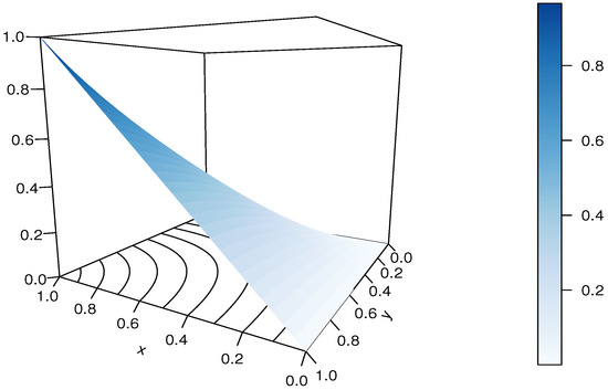
Figure 5. Plots of the shapes and contours of the SRP copula for $\alpha =-1/2$.

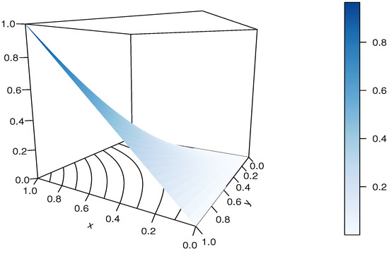
Figure 6. Plots of the shapes and contours of the SRP copula for $\alpha =1$.

These figures show various shapes of the SRP copula. The influence of $\alpha$ on them is significant.

The SRP copula density is calculated as

$$\begin{array}{cc}\hfill c_{\alpha }(x,y)& ={\partial }_{x,y}{C}_{\alpha }(x,y)=\frac{{\alpha }^4{x}^3{y}^3+3{\alpha }^3{x}^2{y}^2+4{\alpha }^{2}xy+\alpha x(2-y)+2\alpha y+1}{(1+\alpha ){(1+\alpha xy)}^3},(x,y)\in {[0,1]}^2.\hfill \end{array}$$

In order to visualize the shapes of this function, the plots are presented in Figure 7 and Figure 8, again for $\alpha =-1/2$ and $\alpha =1$, respectively.

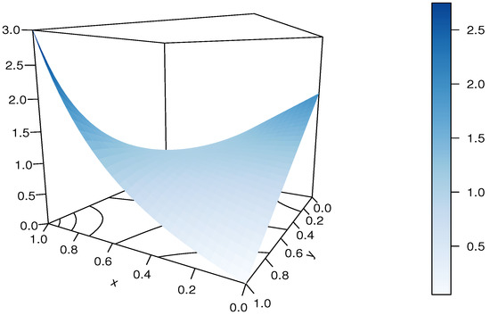
Figure 7. Plots of the shapes and contours of the SRP copula density for $\alpha =-1/2$.

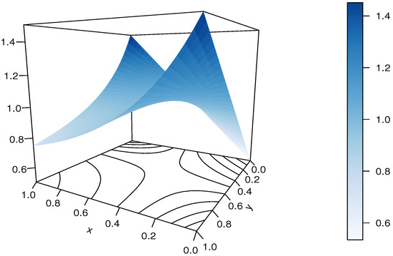
Figure 8. Plots of the shapes and contours of the SRP copula density for $\alpha =1$.

In these figures, the SRP copula density has entirely diverse shapes, demonstrating a certain degree of dependent flexibility. Once more, the influence of $\alpha$ on these shapes is essential.

As a last function of interest, the SRP survival copula is obtained as

$$\begin{array}{cc}\hfill & {\widehat{C}}_{\alpha }(x,y)=x+y-1+C_{\alpha }(1-x,1-y)\hfill \\ \hfill & =x+y-1+(1-x)(1-y)\frac{\left[1+\alpha (1-x)\right]\left[1+\alpha (1-y)\right]}{(1+\alpha )\left[1+\alpha (1-x)(1-y)\right]},(x,y)\in {[0,1]}^2.\hfill \end{array}$$

It is a fresh ratio-copula to be included in the literature.

3.2. Properties

Some essential features of the SRP copula are now presented. The SRP copula is obviously diagonally symmetric because $C_{\alpha }(x,y)=C_{\alpha }(y,x)$ for any $(x,y)\in {[0,1]}^2$. It is not Archimedean, because, for $\alpha =1$ (for instance), it is not associative. Indeed, we have

$$\begin{array}{c}\hfill C_{\alpha }\left[\frac{1}{4},C_{\alpha }\left(\frac{1}{2},\frac{1}{3}\right)\right]=0.02463054\ne 0.02470172=C_{\alpha }\left[C_{\alpha }\left(\frac{1}{4},\frac{1}{2}\right),\frac{1}{3}\right].\end{array}$$

The SRP copula is not radially symmetric because there exists $(x,y)$ such that ${\widehat{C}}_{\alpha }(x,y)\ne C_{\alpha }(x,y)$.

The Fréchet–Hoeffding bounds obviously hold.

Remark 4.

The inequalities that follow, which may be of independent importance, can be deduced from the Fréchet–Hoeffding bounds: For $\alpha \ge -1/2$ and any $(x,y)\in {[0,1]}^2$, we have

$$max(x+y-1,0)(1+\alpha )(1+\alpha xy)\le xy(1+\alpha x)(1+\alpha y)\le min(x,y)(1+\alpha )(1+\alpha xy).$$

Lemma 5.

For $\alpha \in [-1/2,0)$, the SRP copula is positively quadrant dependent, i.e., $C_{\alpha }(x,y)\ge xy$ for any $(x,y)\in {[0,1]}^2$. For $\alpha \in (0,1]$, it is negatively quadrant dependent, i.e., $C_{\alpha }(x,y)\le xy$ for any $(x,y)\in {[0,1]}^2$.

Proof. 

Let us remark that

$${\partial }_{\alpha }{C}_{\alpha }(x,y)=-xy(1-x)(1-y)\frac{1-{\alpha }^{2}xy}{{(1+\alpha )}^2{(1+\alpha xy)}^2}.$$

For $\alpha \in [-1/2,1]$ and any $(x,y)\in {[0,1]}^2$, we have $1-{\alpha }^{2}xy\ge 0$, implying that ${\partial }_{\alpha }{C}_{\alpha }(x,y)\le 0$. Therefore, $C_{\alpha }(x,y)$ is a decreasing function with respect to $\alpha$ for $\alpha \in [-1/2,1]$. Then, for $\alpha \in [-1/2,0)$ and any $(x,y)\in {[0,1]}^2$, we have $C_{\alpha }(x,y)\ge C_0(x,y)=xy$, and, for $\alpha \in (0,1]$, we have $C_{\alpha }(x,y)\le C_0(x,y)=xy$. This concludes the proof. □

For $\alpha \in [-1/2,1)$ and any $(x,y)\in {[0,1)}^2$, by using the geometric series formula, the following power decomposition is obtained:

$$C_{\alpha }(x,y)=\sum _{i=0}^{\infty }{\zeta }_i(1+\alpha x)(1+\alpha y)x^{i+1}{y}^{i+1},$$

where ${\zeta }_i={(-1)}^i{\alpha }^i/(1+\alpha )$.

The SRP copula density can be expanded as

$$c_{\alpha }(x,y)=\sum _{i=0}^{\infty }{\zeta }_i[2i{x}^i{y}^i+\alpha (3i+1)x^i{y}^{i+1}+\alpha (3i+1)x^{i+1}{y}^i+{\alpha }^2(4i+3)x^{i+1}{y}^{i+1}].$$

This formula can be used to expand and approximate various moment measures. Let us now investigate the possible tail dependence of the SRP copula. Using standard limit techniques, we have

$${\lambda }_L=\underset{x\to 0}{lim}\frac{C_{\alpha }(x,x)}{x}=\underset{x\to 0}{lim}x\frac{{(1+\alpha x)}^2}{(1+\alpha )(1+\alpha x^2)}=0$$

and

$${\lambda }_U=\underset{x\to 1}{lim}\frac{1-2x+C_{\alpha }(x,x)}{1-x}=\underset{x\to 1}{lim}\frac{1-2x+x^2{(1+\alpha x)}^2/\left[(1+\alpha )(1+\alpha x^2)\right]}{1-x}=0.$$

The SRP copula hence lacks tail dependence.

The medial correlation of the SRP copula is represented as

$$M=4C_{\alpha }\left(\frac{1}{2},\frac{1}{2}\right)-1=\frac{{(2+\alpha )}^2}{(1+\alpha )(4+\alpha )}-1.$$

The rho of Spearman of the SRP copula is defined by

$$\rho =12{\int }_0^1{\int }_0^1{C}_{\alpha }(x,y)dxdy-3=12{\int }_0^1{\int }_0^{1}xy\frac{(1+\alpha x)(1+\alpha y)}{(1+\alpha )(1+\alpha xy)}dxdy-3.$$

Unfortunately, unlike the RP copula, no closed form expression for $\rho$ exists. We thus propose a numerical analysis in Table 2 by determining its numerical values for a certain grid of values for $\alpha$, including positive and negative values.

Table 2. Values of the rho of Spearman of the SRP copula for a grid of values for $\alpha$.

$\alpha$	−0.5	−0.3	−0.1	0.0	0.6	1.2	1.8	2.4	3.0
$\rho$	0.3848	0.1549	0.038	0	−0.1095	−0.1429	−0.1536	−0.1556	−0.1539

This table demonstrates that the rho of Spearman varies from $-0.16$ to $0.39$. Thus, the SRP copula is ideal to analyze weak-negative or moderate-positive dependence.

The SRP copula has the ability to define new two-dimensional parametric distributional models, with a plethora of possible applications. They are based on the following two-dimensional cumulative distribution function:

$$H_{\alpha }(x,y)=C_{\alpha }[F\left(x\right),G\left(y\right)]=F\left(x\right)G\left(y\right)\frac{[1+\alpha F(x\left)\right][1+\alpha G(y\left)\right]}{(1+\alpha )[1+\alpha F(x\left)G\right(y\left)\right]},(x,y)\in {\mathbb{R}}^2,$$

where $F\left(x\right)$ and $G\left(x\right)$ denote two uni-dimensional cumulative distribution functions.

4. Ratio-Sine Copula

The ratio-copula scheme in Equation (3) is used with trigonometric functions for $\varphi \left(x\right)$ in the current and next sections.

4.1. Presentation

The result below considers the copula form in Equation (3), with $\varphi \left(x\right)=sin\left(\alpha x\right)$, where $\alpha$ denotes a tuning parameter.

Proposition 3.

The following two-dimensional function represents a valid copula:

$$\begin{array}{c}\hfill C_{\alpha }(x,y)=xy\frac{sin\left(\alpha x\right)sin\left(\alpha y\right)}{sin\left(\alpha \right)sin\left(\alpha xy\right)},(x,y)\in {[0,1]}^2,\end{array}$$

(6)

for $\alpha \in [-\pi /2,\pi /2]\left\{0\right\}$, and $C_{\alpha }(x,y)=xy$ for $\alpha =0$.

An alternative multiplicative expression is

$$C_{\alpha }(x,y)=xycsc\left(\alpha \right)sin\left(\alpha x\right)sin\left(\alpha y\right)csc\left(\alpha xy\right),$$

where $csc\left(u\right)=1/sin\left(u\right)$ for any $u\in \mathbb{R}\{k\pi ;k\in \mathbb{Z}\}$.

Proof. 

First of all, since the sine function is an odd function, let us remark that $C_{\alpha }(x,y)=C_{-\alpha }(x,y)$. Therefore, we can restrict our study for $\alpha \in (0,\pi /2]$ only. With this in mind, the rest of the proof is based on Definition 1, and limit, differentiation, well-chosen factorization techniques, and trigonometric inequalities.

(i) For any $x\in [0,1]$, we have

$$C_{\alpha }(x,0)=\underset{y\to 0}{lim}xy\frac{sin\left(\alpha x\right)sin\left(\alpha y\right)}{sin\left(\alpha \right)sin\left(\alpha xy\right)}=\underset{y\to 0}{lim}y\frac{sin\left(\alpha x\right)}{sin\left(\alpha \right)}=0.$$

Using a similar limit technique, for any $y\in [0,1]$, we obtain $C_{\alpha }(0,y)=0$.

(ii) For any $x\in [0,1]$, we have

$$C_{\alpha }(x,1)=x\times 1\times \frac{sin\left(\alpha x\right)sin(\alpha \times 1)}{sin\left(\alpha \right)sin(\alpha x\times 1)}=x.$$

Similarly, for any $y\in [0,1]$, we have $C_{\alpha }(1,y)=y$.

(iii) For any $(x,y)\in {[0,1]}^2$, using standard differentiation techniques and appropriate factorizations, we have

$$\begin{array}{cc}\hfill & {\partial }_{x,y}{C}_{\alpha }(x,y)=csc\left(\alpha \right)csc\left(\alpha xy\right)\{sin\left(\alpha x\right)\left[sin\left(\alpha y\right)f\left(\alpha xy\right)+\alpha ycos\left(\alpha y\right)g\left(\alpha xy\right)\right]\hfill \\ \hfill & +\alpha xcos\left(\alpha x\right)\left(sin\left(\alpha y\right)g\left(\alpha xy\right)+\alpha ycos\left(\alpha y\right)\right)\},\hfill \end{array}$$

where

$$f\left(u\right)=u^2{cot}^2\left(u\right)+u^2{csc}^2\left(u\right)-3ucot\left(u\right)+1$$

and

$$g\left(u\right)=1-ucot\left(u\right),$$

for $u\in (0,\pi /2]$. Since, for $\alpha \in (0,\pi /2]$ and any $(x,y)\in {[0,1]}^2$, we have $sin\left(\alpha \right)>0$, $csc\left(\alpha xy\right)\ge 0$, $sin\left(\alpha x\right)\ge 0$, $cos\left(\alpha x\right)\ge 0$, $sin\left(\alpha y\right)\ge 0$, and $cos\left(\alpha y\right)\ge 0$. Hence, in order to prove (iii), we need to prove that, for any $u\in (0,\pi /2]$, $f\left(u\right)\ge 0$ and $g\left(u\right)\ge 0$. Let us begin with $g\left(u\right)$. The following inequality is well-known: $sin\left(u\right)\ge ucos\left(u\right)$ for any $u\in [0,\pi /2]$. Therefore, we have

$$\begin{array}{c}\hfill g\left(u\right)=csc\left(u\right)[sin(u)-ucos(u\left)\right]\ge 0.\end{array}$$

On the other hand, for $f\left(u\right)$, the following decomposition holds:

$$\begin{array}{cc}\hfill f\left(u\right)& =[u^2{cot}^2\left(u\right)-2ucot\left(u\right)+1]+[u^2{csc}^2\left(u\right)-1]+[1-ucot\left(u\right)]\hfill \\ \hfill & ={(ucot\left(u\right)-1)}^2+{csc}^2\left(u\right)(u^2-{sin}^2\left(u\right))+g\left(u\right).\hfill \end{array}$$

Since $sin\left(u\right)\le u$ for any $u\in [0,\pi /2]$ and $g\left(u\right)\ge 0$, we have $f\left(u\right)\ge 0$. As a result of the inequalities above, we establish that

$${\partial }_{x,y}{C}_{\alpha }(x,y)\ge 0.$$

The point (iii) is proved.

The proof of the proposition ends. □

For the purpose of this paper, the copula defined in Equation (6) is called the ratio-sine (RS) copula. It belongs to the family of trigonometric copulas, which have gained a lot of attention these last few years (see, for instance, [10,12,13,28]). They can be used to uncover dependencies hidden in variables based on circular data (see [28]).

Plots of the RS copula are presented in Figure 9 and Figure 10, for $\alpha =-\pi /2$ and $\alpha =\pi /3$ (arbitrarily chosen in the admissible domain), respectively.

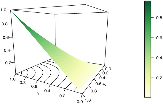
Figure 9. Plots of the shapes and contours of the RS copula for $\alpha =-\pi /2$.

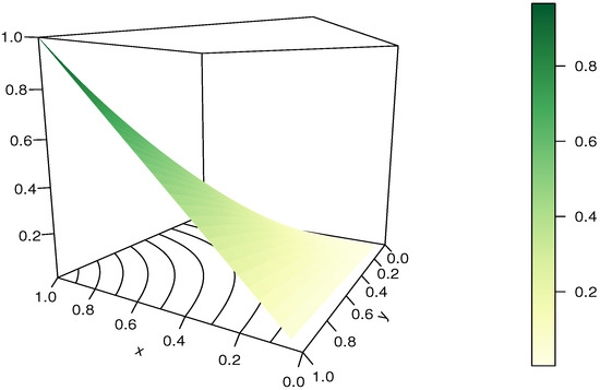
Figure 10. Plots of the shapes and contours of the RS copula for $\alpha =\pi /3$.

From these figures, different shapes and contours in particular are observed. The impact of $\alpha$ on them is clear.

The RS copula density is calculated as

$$\begin{array}{cc}\hfill c_{\alpha }(x,y)& ={\partial }_{x,y}{C}_{\alpha }(x,y)=csc\left(\alpha \right)csc\left(\alpha xy\right)\{sin\left(\alpha x\right)\left[sin\left(\alpha y\right)f\left(\alpha xy\right)+\alpha ycos\left(\alpha y\right)g\left(\alpha xy\right)\right]\hfill \\ \hfill & +\alpha xcos\left(\alpha x\right)\left(sin\left(\alpha y\right)g\left(\alpha xy\right)+\alpha ycos\left(\alpha y\right)\right)\},(x,y)\in {[0,1]}^2,\hfill \end{array}$$

where

$$f\left(u\right)=u^2{cot}^2\left(u\right)+u^2{csc}^2\left(u\right)-3ucot\left(u\right)+1$$

and

$$g\left(u\right)=1-ucot\left(u\right),$$

for $u\in (0,\pi /2]$. The shapes of this function are important to understand the modeling possibilities of the RS copula. In this regard, plots of this function are presented in Figure 11 and Figure 12, again for $\alpha =-\pi /2$ and $\alpha =\pi /3$, respectively.

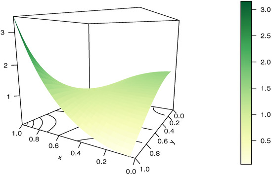
Figure 11. Plots of the shapes and contours of the RS copula density for $\alpha =-\pi /2$.

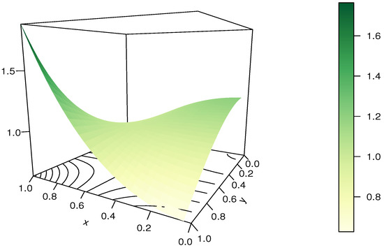
Figure 12. Plots of the shapes and contours of the RS copula density for $\alpha =\pi /3$.

The shapes of the RS copula density are completely different in these figures, illustrating a kind of dependence flexibility. Again, the influence of $\alpha$ on these shapes is crucial.

As a last function of interest, the RS survival copula is obtained as

$$\begin{array}{cc}\hfill & {\widehat{C}}_{\alpha }(x,y)=x+y-1+C_{\alpha }(1-x,1-y)\hfill \\ \hfill & =x+y-1+(1-x)(1-y)\frac{sin\left[\alpha \right(1-x\left)\right]sin\left[\alpha \right(1-y\left)\right]}{sin\left(\alpha \right)sin\left[\alpha \right(1-x\left)\right(1-y\left)\right]},(x,y)\in {[0,1]}^2.\hfill \end{array}$$

It is also a new copula to add to the existing literature.

4.2. Properties

Some key characteristics of the RS copula are now discussed. Clearly, the RS copula is diagonally symmetric because $C_{\alpha }(x,y)=C_{\alpha }(y,x)$ for any $(x,y)\in {[0,1]}^2$. It is not Archimedean, because, for $\alpha =\pi /2$ (for instance), it is not associative. Indeed, we have

$$\begin{array}{c}\hfill C_{\alpha }\left[\frac{1}{4},C_{\alpha }\left(\frac{1}{2},\frac{1}{3}\right)\right]=0.08539428\ne 0.08574002=C_{\alpha }\left[C_{\alpha }\left(\frac{1}{4},\frac{1}{2}\right),\frac{1}{3}\right].\end{array}$$

To the best of our knowledge, the RS copula is one of the rare non-Archimedean copulas based on a ratio of trigonometric functions.

The RS copula is not radially symmetric because there exists $(x,y)$ such that ${\widehat{C}}_{\alpha }(x,y)\ne C_{\alpha }(x,y)$.

Of course, as for any copula, the Fréchet–Hoeffding bounds hold.

Remark .

From the Fréchet–Hoeffding bounds, the following inequalities can be derived, which can be of independent interest: For $\alpha \in [-\pi /2,\pi /2]$ and any $(x,y)\in {[0,1]}^2$, we have

$$max(x+y-1,0)sin\left(\alpha \right)sin\left(\alpha xy\right)\le xysin\left(\alpha x\right)sin\left(\alpha y\right)\le min(x,y)sin\left(\alpha \right)sin\left(\alpha xy\right).$$

Let us now investigate the possible tail dependence of the RS copula. Using standard limit techniques, we establish that

$${\lambda }_L=\underset{x\to 0}{lim}\frac{C_{\alpha }(x,x)}{x}=\underset{x\to 0}{lim}x\frac{{sin}^2\left(\alpha x\right)}{sin\left(\alpha \right)sin\left(\alpha x^2\right)}=0$$

and

$${\lambda }_U=\underset{x\to 1}{lim}\frac{1-2x+C_{\alpha }(x,x)}{1-x}=\underset{x\to 1}{lim}\frac{1-2x+x^2{sin}^2\left(\alpha x\right)/[sin\left(\alpha \right)sin\left(\alpha x^2\right)]}{1-x}=0.$$

It follows that the RS copula has no tail dependence.

The medial correlation of the RS copula is simply indicated as

$$M=4C_{\alpha }\left(\frac{1}{2},\frac{1}{2}\right)-1=\frac{{sin}^2(\alpha /2)}{sin\left(\alpha \right)sin(\alpha /4)}-1.$$

The rho of Spearman of the RS copula is defined by

$$\rho =12{\int }_0^1{\int }_0^1{C}_{\alpha }(x,y)dxdy-3=12{\int }_0^1{\int }_0^{1}xy\frac{sin\left(\alpha x\right)sin\left(\alpha y\right)}{sin\left(\alpha \right)sin\left(\alpha xy\right)}dxdy-3.$$

Unfortunately, there is no closed form expression for $\rho$. We thus propose a numerical analysis. To this aim, Table 3 determines the numerical values of $\rho$ for a certain grid of values for $\alpha$.

Table 3. Values of the rho of Spearman of the RS copula for a grid of values for $\alpha$.

$\alpha$	0.01	0.31	0.61	0.91	1.21	1.51
$\rho$	0	0.0121	0.0482	0.1125	0.2133	0.3665

This table demonstrates that the rho of Spearman varies from 0 to a little bit more than $0.36$. Thus, the RS copula is ideal to analyze the middle dependence.

The RS copula has the ability to define new parametric two-dimensional distributional models based on the following two-dimensional cumulative distribution function:

$$H_{\alpha }(x,y)=C_{\alpha }[F\left(x\right),G\left(y\right)]=F\left(x\right)G\left(y\right)\frac{sin\left[\alpha F\right(x\left)\right]sin\left[\alpha G\right(y\left)\right]}{sin\left(\alpha \right)sin\left[\alpha F\right(x\left)G\right(y\left)\right]},(x,y)\in {\mathbb{R}}^2,$$

where $F\left(x\right)$ and $G\left(x\right)$ denote two uni-dimensional cumulative distribution functions.

5. Ratio-Arctangent Copula

5.1. Presentation

The result below considers the copula form in Equation (3), with $\varphi \left(x\right)=arctan\left(\alpha x\right)$, where $\alpha$ denotes a tuning parameter.

Proposition 4.

The following two-dimensional function represents a valid copula:

$$\begin{array}{c}\hfill C_{\alpha }(x,y)=xy\frac{arctan\left(\alpha x\right)arctan\left(\alpha y\right)}{arctan\left(\alpha \right)arctan\left(\alpha xy\right)},(x,y)\in {[0,1]}^2,\end{array}$$

(7)

for $\alpha \in \mathbb{R}\left\{0\right\}$, and $C_{\alpha }(x,y)=xy$ for $\alpha =0$.

Proof. 

First of all, since the arctan function is an odd function, let us remark that $C_{\alpha }(x,y)=C_{-\alpha }(x,y)$. Therefore, we can restrict our study for $\alpha >0$ only. With this in mind, the rest of the proof is based on Definition 1, and limit, differentiation, well-chosen factorization techniques, and trigonometric inequalities.

(i) For any $x\in [0,1]$, we have

$$C_{\alpha }(x,0)=\underset{y\to 0}{lim}xy\frac{arctan\left(\alpha x\right)arctan\left(\alpha y\right)}{arctan\left(\alpha \right)arctan\left(\alpha xy\right)}=\underset{y\to 0}{lim}y\frac{arctan\left(\alpha x\right)}{arctan\left(\alpha \right)}=0.$$

Using a similar limit technique, for any $y\in [0,1]$, we obtain $C_{\alpha }(0,y)=0$.

(ii) For any $x\in [0,1]$, we have

$$C_{\alpha }(x,1)=x\times 1\times \frac{arctan\left(\alpha x\right)arctan(\alpha \times 1)}{arctan\left(\alpha \right)arctan(\alpha x\times 1)}=x.$$

Similarly, for any $y\in [0,1]$, $C_{\alpha }(1,y)=y$.

(iii) For any $(x,y)\in {[0,1]}^2$, using standard differentiation techniques and appropriate factorizations, we have

$$\begin{array}{cc}\hfill & {\partial }_{x,y}{C}_{\alpha }(x,y)=\frac{1}{arctan\left(\alpha \right){arctan}^3\left(\alpha xy\right)}\times \hfill \\ \hfill & \{\frac{1}{1+{\alpha }^2{x}^2}\left[\alpha xarctan\left(\alpha xy\right)\left(arctan\left(\alpha y\right)f\left(\alpha xy\right)+\frac{\alpha yarctan\left(\alpha xy\right)}{1+{\alpha }^2{y}^2}\right)\right]\hfill \\ \hfill & +\frac{arctan\left(\alpha x\right)}{{(1+{\alpha }^2{x}^2{y}^2)}^2}(\frac{\alpha y}{1+{\alpha }^2{y}^2}{(1+{\alpha }^2{x}^2{y}^2)}^{2}arctan\left(\alpha xy\right)f\left(\alpha xy\right)\hfill \\ \hfill & +arctan\left(\alpha y\right)g\left(\alpha xy\right)\left)\right\},\hfill \end{array}$$

where

$$f\left(u\right)=arctan\left(u\right)-\frac{u}{1+u^2}$$

and

$$g\left(u\right)=2u^2-u(u^2+3)arctan\left(u\right)+{(1+u^2)}^2{arctan}^2\left(u\right),$$

for $u>0$.

Since, for $\alpha >0$ and any $(x,y)\in {[0,1]}^2$, we have $arctan\left(\alpha \right)>0$, $arctan\left(\alpha xy\right)\ge 0$, $arctan\left(\alpha x\right)\ge 0$, and $arctan\left(\alpha y\right)\ge 0$. Hence, in order to prove (iii), we need to prove that, for any $u>0$, $f\left(u\right)\ge 0$ and $g\left(u\right)\ge 0$.

Let us begin with $f\left(u\right)$. The following inequality is well-known: $arctan\left(u\right)\ge u/(1+u^2)$ for any $u>0$. Therefore, it is immediate that $f\left(u\right)\ge 0$.

For $g\left(u\right)$, the developments are more technical. We can write

$$\begin{array}{cc}\hfill g\left(u\right)& =2u(u-arctan\left(u\right))+{(1+u^2)}^{2}arctan\left(u\right)f\left(u\right).\hfill \end{array}$$

Since $arctan\left(u\right)\le u$ for any $u\ge 0$ and $f\left(u\right)\ge 0$, we have $g\left(u\right)\ge 0$. As a result of the inequalities above, we establish that

$${\partial }_{x,y}{C}_{\alpha }(x,y)\ge 0.$$

The point (iii) is proved.

The proof of the proposition ends. □

For the purpose of this paper, the copula defined in Equation (7) is called the ratio-arctangent (RA) copula. As with the RS copula, it belongs to the family of trigonometric copulas, enriching the literature in this regard.

Plots of the RA copula are presented in Figure 13 and Figure 14, for $\alpha =-1/2$ and $\alpha =1$ (arbitrarily chosen in the admissible domain), respectively.

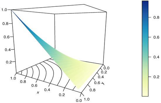
Figure 13. Plots of the shapes and contours of the RA copula for $\alpha =-1/2$.

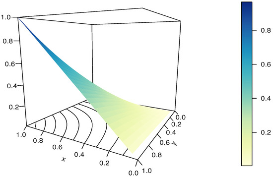
Figure 14. Plots of the shapes and contours of the RA copula for $\alpha =1$.

From these figures, different shape morphologies are observed for the RA copula. The impact of $\alpha$ on them is clear.

The RA copula density is calculated as

$$\begin{array}{cc}\hfill & c_{\alpha }(x,y)={\partial }_{x,y}{C}_{\alpha }(x,y)=\frac{1}{arctan\left(\alpha \right){arctan}^3\left(\alpha xy\right)}\times \hfill \\ \hfill & \{\frac{1}{1+{\alpha }^2{x}^2}\left[\alpha xarctan\left(\alpha xy\right)\left(arctan\left(\alpha y\right)f\left(\alpha xy\right)+\frac{\alpha yarctan\left(\alpha xy\right)}{1+{\alpha }^2{y}^2}\right)\right]\hfill \\ \hfill & +\frac{arctan\left(\alpha x\right)}{{(1+{\alpha }^2{x}^2{y}^2)}^2}(\frac{\alpha y}{1+{\alpha }^2{y}^2}{(1+{\alpha }^2{x}^2{y}^2)}^{2}arctan\left(\alpha xy\right)f\left(\alpha xy\right)\hfill \\ \hfill & +arctan\left(\alpha y\right)g\left(\alpha xy\right)\left)\right\},(x,y)\in {[0,1]}^2,\hfill \end{array}$$

where

$$f\left(u\right)=arctan\left(u\right)-\frac{u}{1+u^2}$$

and

$$g\left(u\right)=2u^2-u(u^2+3)arctan\left(u\right)+{(1+u^2)}^2{arctan}^2\left(u\right),$$

for $u>0$.

Plots of the RA copula density are presented in Figure 15 and Figure 16, again for $\alpha =-1/2$ and $\alpha =1$, respectively.

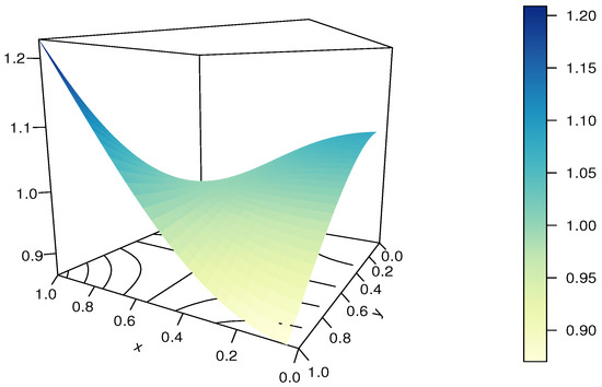
Figure 15. Plots of the shapes and contours of the RA copula density for $\alpha =-1/2$.

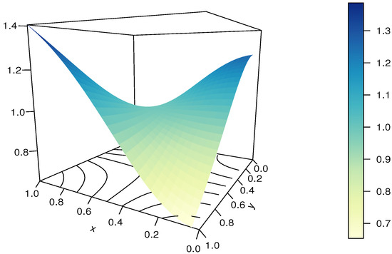
Figure 16. Plots of the shapes and contours of the RA copula density for $\alpha =1$.

The shapes of the RA copula density are completely different in these figures, illustrating a kind of dependence flexibility. Again, the effect of $\alpha$ on these shapes is crucial. Further results on this subject will be proved theoretically.

As a last function of interest, the RA survival copula is obtained as

$$\begin{array}{cc}\hfill & {\widehat{C}}_{\alpha }(x,y)=x+y-1+C_{\alpha }(1-x,1-y)\hfill \\ \hfill & =x+y-1+(1-x)(1-y)\frac{arctan\left[\alpha \right(1-x\left)\right]arctan\left[\alpha \right(1-y\left)\right]}{arctan\left(\alpha \right)arctan\left[\alpha \right(1-x\left)\right(1-y\left)\right]},(x,y)\in {[0,1]}^2.\hfill \end{array}$$

Additionally, it is a fresh copula to be included in the literature.

5.2. Properties

Now, some essential features of the RA copula are explained. Clearly, the RA copula is diagonally symmetric because $C_{\alpha }(x,y)=C_{\alpha }(y,x)$ for any $(x,y)\in {[0,1]}^2$. It is not Archimedean, since, for $\alpha =10$ (for instance), the associativity condition is not satisfied; we have

$$\begin{array}{c}\hfill C_{\alpha }\left[\frac{1}{4},C_{\alpha }\left(\frac{1}{2},\frac{1}{3}\right)\right]=0.09494162\ne 0.09401747=C_{\alpha }\left[C_{\alpha }\left(\frac{1}{4},\frac{1}{2}\right),\frac{1}{3}\right].\end{array}$$

The RA copula is one of the few non-Archimedean copulas based on a ratio of trigonometric functions, as far as we are aware.

The RA copula is not radially symmetric because there exists $(x,y)$ such that ${\widehat{C}}_{\alpha }(x,y)\ne C_{\alpha }(x,y)$.

Of course, as for any copula, the Fréchet–Hoeffding bounds hold.

Remark 6.

The inequalities that follow, which may be of independent interest, can be derived from the Fréchet–Hoeffding bounds: For $\alpha \in \mathbb{R}$ and any $(x,y)\in {[0,1]}^2$, we have

$$\begin{array}{cc}\hfill max(x+y-1,0)arctan\left(\alpha \right)arctan\left(\alpha xy\right)& \le xyarctan\left(\alpha x\right)arctan\left(\alpha y\right)\hfill \\ \hfill & \le min(x,y)arctan\left(\alpha \right)arctan\left(\alpha xy\right).\hfill \end{array}$$

Let us now investigate the possible tail dependence of the RA copula. Using standard limit techniques, we have

$${\lambda }_L=\underset{x\to 0}{lim}\frac{C_{\alpha }(x,x)}{x}=\underset{x\to 0}{lim}x\frac{{arctan}^2\left(\alpha x\right)}{arctan\left(\alpha \right)arctan\left(\alpha x^2\right)}=0$$

and

$${\lambda }_U=\underset{x\to 1}{lim}\frac{1-2x+C_{\alpha }(x,x)}{1-x}=\underset{x\to 1}{lim}\frac{1-2x+x^2{arctan}^2\left(\alpha x\right)/[arctan\left(\alpha \right)arctan\left(\alpha x^2\right)]}{1-x}=0.$$

It follows that the RA copula has no tail dependence.

The medial correlation of the RA copula is simply indicated as

$$M=4C_{\alpha }\left(\frac{1}{2},\frac{1}{2}\right)-1=\frac{{arctan}^2(\alpha /2)}{arctan\left(\alpha \right)arctan(\alpha /4)}-1.$$

The rho of Spearman of the RA copula is defined by

$$\rho =12{\int }_0^1{\int }_0^1{C}_{\alpha }(x,y)dxdy-3=12{\int }_0^1{\int }_0^{1}xy\frac{arctan\left(\alpha x\right)arctan\left(\alpha y\right)}{arctan\left(\alpha \right)arctan\left(\alpha xy\right)}dxdy-3.$$

Unfortunately, $\rho$ has no closed form expression. So, we suggest an analysis using numeric values. Table 4 determines numerical values of $\rho$ for a certain grid of values for $\alpha$.

Table 4. Values of the rho of Spearman of the RA copula for a grid of values for $\alpha$.

$\alpha$	0.01	0.51	1.01	1.51	2.01	2.51	3.01	3.51	4.01	4.51
$\rho$	0	0.0551	0.1495	0.2197	0.2594	0.2781	0.284	0.2827	0.2772	0.2695

This table demonstrates that the rho of Spearman varies from 0 to a little bit more than $0.28$. Thus, the RA copula is ideal to analyze the middle dependence.

The RA copula can create new parametric distributional models with a wide range of potential uses. They are based on the following two-dimensional cumulative distribution function:

$$H_{\alpha }(x,y)=C_{\alpha }[F\left(x\right),G\left(y\right)]=F\left(x\right)G\left(y\right)\frac{arctan\left[\alpha F\right(x\left)\right]arctan\left[\alpha G\right(y\left)\right]}{arctan\left(\alpha \right)arctan\left[\alpha F\right(x\left)G\right(y\left)\right]},(x,y)\in {\mathbb{R}}^2,$$

where $F\left(x\right)$ and $G\left(x\right)$ denote two uni-dimensional cumulative distribution functions.

6. Ratio-Logarithmic Copula

This section investigates a logarithmic copula based on Equation (3). It can be viewed as the logarithmic-copula counterpart of the CC copula.

6.1. Presentation

The result below considers the copula form in Equation (3), with $\varphi \left(x\right)=log(1+\alpha x)$, where $\alpha$ denotes a tuning parameter.

Proposition 5.

The following two-dimensional function represents a valid copula:

$$\begin{array}{c}\hfill C_{\alpha }(x,y)=xy\frac{log(1+\alpha x)log(1+\alpha y)}{log(1+\alpha )log(1+\alpha xy)},(x,y)\in {[0,1]}^2,\end{array}$$

(8)

for $\alpha >0$, and $C_{\alpha }(x,y)=xy$ for $\alpha =0$.

Proof. 

As the copulas presented before, the proof is based on Definition 1, and limit, differentiation, well-chosen factorization techniques, and logarithmic inequalities.

(i) For any $x\in [0,1]$, we have

$$C_{\alpha }(x,0)=\underset{y\to 0}{lim}xy\frac{log(1+\alpha x)log(1+\alpha y)}{log(1+\alpha )log(1+\alpha xy)}=\underset{y\to 0}{lim}y\frac{log(1+\alpha x)}{log(1+\alpha )}=0.$$

Using a similar limit technique, for any $y\in [0,1]$, we obtain $C_{\alpha }(0,y)=0$.

(ii) For any $x\in [0,1]$, we have

$$C_{\alpha }(x,1)=x\times 1\times \frac{log(1+\alpha x)log(1+\alpha \times 1)}{log(1+\alpha )log(1+\alpha x\times 1)}=x.$$

Similarly, for any $y\in [0,1]$, we have $C_{\alpha }(1,y)=y$.

(iii) For any $(x,y)\in {[0,1]}^2$, using standard differentiation techniques and appropriate factorizations, we have

$$\begin{array}{cc}\hfill & {\partial }_{x,y}{C}_{\alpha }(x,y)=\frac{1}{log(1+\alpha ){(1+\alpha xy)}^2{log}^3(1+\alpha xy)}\times \hfill \\ \hfill & \{log(1+\alpha x\left)\right[log(1+\alpha y)f\left(\alpha xy\right)\hfill \\ \hfill & +\frac{1}{1+\alpha y}\left(\alpha y(1+\alpha xy)log(1+\alpha xy)g\left(\alpha xy\right)\right)]\hfill \\ \hfill & +\frac{\alpha x}{(1+\alpha x)(1+\alpha y)}(1+\alpha xy)log(1+\alpha xy)\times \hfill \\ \hfill & \left(\alpha y(1+\alpha xy)log(1+\alpha xy)+(1+\alpha y)log(1+\alpha y)g\left(\alpha xy\right)\right)\},\hfill \end{array}$$

where

$$f\left(u\right)=2u^2+{(1+u)}^2{log}^2(1+u)-u(2u+3)log(1+u)$$

and

$$g\left(u\right)=(1+u)log(1+u)-u,$$

for $u>0$. Since, for $\alpha >0$ and any $(x,y)\in {[0,1]}^2$, we have $log(1+\alpha )>0$, $log(1+\alpha xy)\ge 0$, $log(1+\alpha x)\ge 0$, and $log(1+\alpha y)\ge 0$. Hence, in order to prove (iii), we need to prove that, for any $u>0$, $f\left(u\right)\ge 0$ and $g\left(u\right)\ge 0$.

Let us begin with $g\left(u\right)$. The following inequality is well-known: $log(1+u)\ge u/(1+u)$ for any $u>0$. Therefore, it is immediate that $g\left(u\right)\ge 0$.

The following inequality is also well-known: $log(1+u)\le u$ for any $u>0$. Therefore,

$$\begin{array}{c}\hfill f\left(u\right)=u[u-log(1+u)]+{[(1+u)log(1+u)-u]}^2\ge 0.\end{array}$$

As a result of the inequalities above, we establish that

$${\partial }_{x,y}{C}_{\alpha }(x,y)\ge 0.$$

The point (iii) is proved.

The proof of the proposition ends. □

For the purpose of this paper, the copula defined in Equation (8) is called the ratio-logarithmic (RL) copula. Plots of the RL copula are presented in Figure 17 and Figure 18, for $\alpha =1$ and $\alpha =100$ (arbitrarily chosen in the admissible domain), respectively.

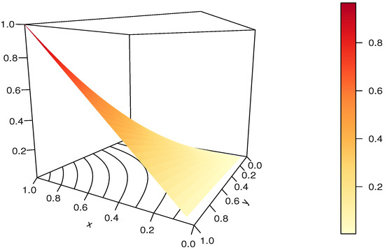
Figure 17. Plots of the shapes and contours of the RL copula for $\alpha =1$.

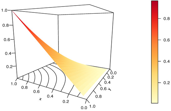
Figure 18. Plots of the shapes and contours of the RL copula for $\alpha =100$.

From these figures, slightly different shapes are observed for the RL copula, but the influence of $\alpha$ seems moderate.

It is conjectured that the RL copula is still valid for some negative values for $\alpha$ (the points (i) and (ii) of Definition 1 remain true), but the related admissible domain for the negative values conducted by the point (iii) of Definition 1 remains a mathematical challenge. Numerical tests validate $\alpha \ge -1/2$ (a bit less in fact). We illustrate this conjecture by a plot of the RL copula for $\alpha =-1/2$ in Figure 19.

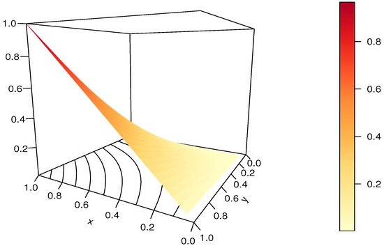
Figure 19. Illustration of the conjecture: plots of the shapes and contours of the RL copula for $\alpha =-1/2$.

The RL copula density is calculated as

$$\begin{array}{cc}\hfill & c_{\alpha }(x,y)={\partial }_{x,y}{C}_{\alpha }(x,y)=\frac{1}{log(1+\alpha ){(1+\alpha xy)}^2{log}^3(1+\alpha xy)}\times \hfill \\ \hfill & \{log(1+\alpha x\left)\right[log(1+\alpha y)f\left(\alpha xy\right)\hfill \\ \hfill & +\frac{1}{1+\alpha y}\left(\alpha y(1+\alpha xy)log(1+\alpha xy)g\left(\alpha xy\right)\right)]\hfill \\ \hfill & +\frac{\alpha x}{(1+\alpha x)(1+\alpha y)}(1+\alpha xy)log(1+\alpha xy)\times \hfill \\ \hfill & \left(\alpha y(1+\alpha xy)log(1+\alpha xy)+(1+\alpha y)log(1+\alpha y)g\left(\alpha xy\right)\right)\},(x,y)\in {[0,1]}^2,\hfill \end{array}$$

where

$$f\left(u\right)=2u^2+{(1+u)}^2{log}^2(1+u)-u(2u+3)log(1+u)$$

and

$$g\left(u\right)=(1+u)log(1+u)-u,$$

for $u>0$. Figure 20 and Figure 21 show plots of the RL copula density for $\alpha =1$ and $\alpha =100$, respectively, to give a better idea of its shape possibilities.

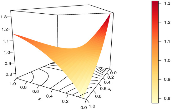
Figure 20. Plots of the shapes and contours of the RL copula density for $\alpha =1$.

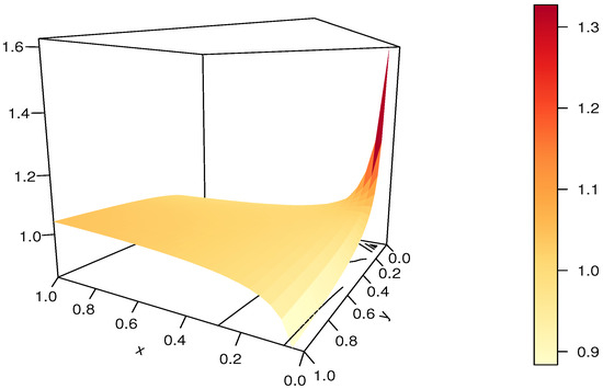
Figure 21. Plots of the shapes and contours of the RL copula density for $\alpha =100$.

The conjecture that the RL copula is still valid for $\alpha \ge -1/2$ is illustrated in Figure 22, with the value $\alpha =-1/2$.

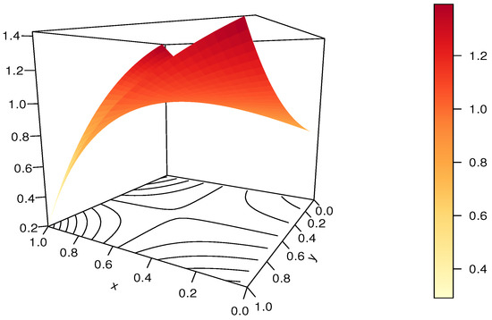
Figure 22. Illustration of the conjecture: plots of the shapes and contours of the RL copula density for $\alpha =-1/2$.

The shapes of the copula density are completely different in these figures, illustrating a kind of dependence flexibility. Again, the impact of $\alpha$ on these shapes is crucial, especially on the extreme points. Further results on this subject will be proved theoretically.

As a last function of interest, the RL survival copula is obtained as

$$\begin{array}{cc}\hfill & {\widehat{C}}_{\alpha }(x,y)=x+y-1+C_{\alpha }(1-x,1-y)\hfill \\ \hfill & =x+y-1+(1-x)(1-y)\frac{log[1+\alpha (1-x\left)\right]log[1+\alpha (1-y\left)\right]}{log(1+\alpha )log[1+\alpha (1-x\left)\right(1-y\left)\right]},(x,y)\in {[0,1]}^2.\hfill \end{array}$$

In the current literature, it represents a novel copula.

6.2. Properties

Now, some essential features of the RL copula are explained. Clearly, the RL copula is diagonally symmetric because $C_{\alpha }(x,y)=C_{\alpha }(y,x)$ for any $(x,y)\in {[0,1]}^2$. It is not Archimedean, since, for $\alpha =10$ (for instance); the associativity condition is violated since

$$\begin{array}{c}\hfill C_{\alpha }\left[\frac{1}{4},C_{\alpha }\left(\frac{1}{2},\frac{1}{3}\right)\right]=0.06690479\ne 0.06689787=C_{\alpha }\left[C_{\alpha }\left(\frac{1}{4},\frac{1}{2}\right),\frac{1}{3}\right].\end{array}$$

We know of just a few non-Archimedean copulas based on a ratio of logarithmic functions, and the RL copula is one of them.

The RL copula is not radially symmetric because there exists $(x,y)$ such that ${\widehat{C}}_{\alpha }(x,y)\ne C_{\alpha }(x,y)$.

Of course, as for any copula, the Fréchet–Hoeffding bounds hold.

Remark 7.

The inequalities that follow, which may be of independent interest, can be derived from the Fréchet–Hoeffding bounds: For $\alpha \ge 0$ and any $(x,y)\in {[0,1]}^2$, we have

$$\begin{array}{cc}\hfill max(x+y-1,0)log(1+\alpha )log(1+\alpha xy)& \le xylog(1+\alpha x)log(1+\alpha y)\hfill \\ \hfill & \le min(x,y)log(1+\alpha )log(1+\alpha xy).\hfill \end{array}$$

Let us now investigate the possible tail dependence of the RL copula. Using standard limit techniques, we have

$${\lambda }_L=\underset{x\to 0}{lim}\frac{C_{\alpha }(x,x)}{x}=\underset{x\to 0}{lim}x\frac{{log}^2(1+\alpha x)}{log(1+\alpha )log(1+\alpha x^2)}=0$$

and

$${\lambda }_U=\underset{x\to 1}{lim}\frac{1-2x+C_{\alpha }(x,x)}{1-x}=\underset{x\to 1}{lim}\frac{1-2x+x^2{log}^2(1+\alpha x)/[log(1+\alpha )log(1+\alpha x^2)]}{1-x}=0.$$

It follows that the RL copula has no tail dependence.

The medial correlation of the RL copula is simply indicated as

$$M=4C_{\alpha }\left(\frac{1}{2},\frac{1}{2}\right)-1=\frac{{log}^2(1+\alpha /2)}{log(1+\alpha )log(1+\alpha /4)}-1.$$

The rho of Spearman of the RL copula is defined by

$$\rho =12{\int }_0^1{\int }_0^1{C}_{\alpha }(x,y)dxdy-3=12{\int }_0^1{\int }_0^{1}xy\frac{log(1+\alpha x)log(1+\alpha y)}{log(1+\alpha )log(1+\alpha xy)}dxdy-3.$$

Unfortunately, no closed form expression for $\rho$ exists. We thus propose a numerical analysis. To this aim, Table 5 determines numerical values of $\rho$ for a certain grid of values for $\alpha$.

Table 5. Values of the rho of Spearman of the RL copula for a grid of values for $\alpha$.

$\alpha$	0.01	0.51	1.01	1.51	2.01	2.51	3.01	3.51	4.01	4.51
$\rho$	0.0017	0.0582	0.0867	0.1028	0.1123	0.118	0.1215	0.1235	0.1246	0.1249

For the conjecture case, Table 6 determines the numerical values of $\rho$ for a certain grid of negative values for $\alpha$.

Table 6. Values of the rho of Spearman of the RL copula for a grid of negative values for $\alpha$.

$\alpha$	−0.50	−0.35	−0.20	−0.05
$\rho$	−0.1451	−0.0833	−0.0403	−0.0087

These tables demonstrate that the rho of Spearman varies from 0 to a little bit more than $0.12$ (and from $-0.14$ to 0 for the conjectured case). Thus, the RL copula is ideal to analyze weak dependence.

New parametric distributional models with a variety of applications can be produced using the RL copula. They are based on the following two-dimensional cumulative distribution function:

$$H_{\alpha }(x,y)=C_{\alpha }[F\left(x\right),G\left(y\right)]=F\left(x\right)G\left(y\right)\frac{log[1+\alpha F(x\left)\right]log[1+\alpha G(y\left)\right]}{log(1+\alpha )log[1+\alpha F(x\left)G\right(y\left)\right]},(x,y)\in {\mathbb{R}}^2,$$

where $F\left(x\right)$ and $G\left(x\right)$ denote two uni-dimensional cumulative distribution functions.

7. A Note on a Multi-Dimensional Approach

Naturally, the notion of copula can be defined for the multi-dimensional case. A standard definition is given below.

Definition 2.

Let $n\ge 2$ be an integer. The function $C:{[0,1]}^n\to [0,1]$ is an (absolutely continuous) n-dimensional copula if and only if

(i) we have $C(x_1,\dots ,x_{i-1},0,x_{i+1},\dots ,x_n)=0$ for any $(x_1,\dots ,x_n)\in {[0,1]}^n$ and $i=1,\dots ,n$.

(ii) we have $C(1,\dots ,1,x,1,\dots ,1)=x$ for any $x\in [0,1]$, and this, in each of the n vector components (the n-dimensional function is equal to x if one vector component is x and all others are equal to 1).

(iii) we have

$${\displaystyle {\partial }_{x_1,\dots ,x_n}C(x_1,\dots ,x_n)\ge 0}$$

for any $(x_1,\dots ,x_n)\in {[0,1]}^n$, where ${\partial }_{x_1,\dots ,x_n}={\partial }^n/\left(\partial x_1\dots \partial x_n\right)$ denotes the mixed n-th order partial derivatives according to $x_1,\dots ,x_n$.

A possible generalization of the copula form suggested in Equation (3) is

$$\begin{array}{c}\hfill C_{\alpha }(x_1,\dots ,x_n)=\left(\prod _{i=1}^n{x}_i\right)\frac{{\prod }_{i=1}^n\varphi \left(x_i\right)}{\varphi {\left(1\right)}^{n-1}\varphi \left({\prod }_{i=1}^n{x}_i\right)},(x_1,\dots ,x_n)\in {[0,1]}^n,\end{array}$$

(9)

where $\varphi$ still denotes a certain uni-dimensional function.

The result below considers the copula form in Equation (3), with $\varphi \left(x\right)=1/(1+\alpha x)$, where $\alpha$ denotes a tuning parameter (or $\varphi \left(x\right)=x^{\beta }/(1+\alpha x)$, where $\beta$ is a tuning parameter that has no effect on the definition of the copula in Equation (9)).

Proposition 6.

Let $n\ge 2$ be an integer. The following n-dimensional function represents a valid copula:

$$\begin{array}{c}\hfill C_{\alpha }(x_1,\dots ,x_n)=\left(\prod _{i=1}^n{x}_i\right)\frac{{(1+\alpha )}^{n-1}\left(1+\alpha {\prod }_{i=1}^n{x}_i\right)}{{\prod }_{i=1}^n(1+\alpha x_i)},(x_1,\dots ,x_n)\in {[0,1]}^n,\end{array}$$

(10)

for $\alpha \ge -1/2^n$.

Proof. 

The proof is based on Definition 2, and limit, differentiation, well-chosen factorization techniques, and polynomial inequalities.

(i) For any $(x_1,\dots ,x_n)\in {[0,1]}^n$, we have

$$C_{\alpha }(0,x_2,\dots ,x_n)=\left(0\times \prod _{i=2}^n{x}_i\right)\frac{{(1+\alpha )}^{n-1}\left(1+\alpha \times 0\times {\prod }_{i=2}^n{x}_i\right)}{(1+\alpha \times 0){\prod }_{i=2}^n(1+\alpha x_i)}=0$$

and, similarly, we have $C_{\alpha }(x_1,\dots ,x_{i-1},0,x_{i+1},\dots ,x_n)=0$ for any $i=2,\dots ,n$.

(ii) For any $x\in [0,1]$, we have

$$C_{\alpha }(x,1,\dots ,1)=x\times 1^{n-1}\times \frac{{(1+\alpha )}^{n-1}\left(1+\alpha x\times 1^{n-1}\right)}{(1+\alpha x\times 1){\prod }_{i=2}^n(1+\alpha \times 1)}=x.$$

More generally, $C_{\alpha }(x_1,\dots ,x_n)$ is equal to x if one vector component is x and all others are equal to 1.

(iii) For any $(x_1,\dots ,x_n)\in {[0,1]}^n$, using differentiation techniques and multiple (non-trivial) factorizations, we have

$$\begin{array}{c}\hfill {\displaystyle {\partial }_{x_1,\dots ,x_n}{C}_{\alpha }(x_1,\dots ,x_n)={(1+\alpha )}^{n-1}\frac{1+\alpha \left({\prod }_{i=1}^n{x}_i\right){\prod }_{i=1}^n(2+\alpha x_i)}{{\prod }_{i=1}^n{(1+\alpha x_i)}^2}.}\end{array}$$

It is clear that, for $\alpha \ge -1/2^n$ and any $(x_1,\dots ,x_n)\in {[0,1]}^n$, we have ${(1+\alpha )}^{n-1}>0$ and ${(1+\alpha x_i)}^2>0$ for any $i=1,\dots ,n$. For $\alpha \ge 0$, it is immediate that $1+\alpha \left({\prod }_{i=1}^n{x}_i\right){\prod }_{i=1}^n$$(2+\alpha x_i)\ge 0$. On the other hand, for $\alpha \in [-1/2^n,0)$, since $2+\alpha x_i\in (0,2]$ for any $i=1,\dots ,n$, we have

$$1+\alpha \left(\prod _{i=1}^n{x}_i\right)\prod _{i=1}^n(2+\alpha x_i)\ge 1+2^n\alpha \left(\prod _{i=1}^n{x}_i\right)\ge 1+2^n\alpha \ge 0.$$

Hence, for $\alpha \ge -1/2^n$, we obtain

$${\displaystyle {\partial }_{x_1,\dots ,x_n}{C}_{\alpha }(x_1,\dots ,x_n)\ge 0.}$$

The point (iii) is proved.

The proof of the proposition ends. □

For the purpose of this paper, the copula defined in Equation (10) is called the generalized RP (GRP) copula. It defines a new n-dimensional copula in the literature. For $n=2$, we obtain the RP copula, and for $n=3$, the following expression is obtained:

$$C_{\alpha }(x,y,z)=xyz\frac{{(1+\alpha )}^2(1+\alpha xyz)}{(1+\alpha x)(1+\alpha y)(1+\alpha z)},(x,y,z)\in {[0,1]}^3.$$

The GRP copula density is given by

$$\begin{array}{cc}\hfill c_{\alpha }(x_1,\dots ,x_n)& {\displaystyle ={\partial }_{x_1,\dots ,x_n}{C}_{\alpha }(x_1,\dots ,x_n)}\hfill \\ \hfill & ={(1+\alpha )}^{n-1}\frac{1+\alpha \left({\prod }_{i=1}^n{x}_i\right){\prod }_{i=1}^n(2+\alpha x_i)}{{\prod }_{i=1}^n{(1+\alpha x_i)}^2},(x_1,\dots ,x_n)\in {[0,1]}^n.\hfill \end{array}$$

For any permutation of $(x_1,\dots ,x_n)$, say $(x_{\sigma \left(1\right)},\dots ,x_{\sigma \left(n\right)})$, we have $C_{\alpha }(x_{\sigma \left(1\right)},\dots ,x_{\sigma \left(n\right)})=C_{\alpha }(x_{},\dots ,x_n)$. As a result, the GRP copula is exchangeable.

Of course, as for any multi-dimensional copula, the Fréchet–Hoeffding bounds hold. Thus, for any $(x_1,\dots ,x_n)\in {[0,1]}^n$, we have

$$max\left(1-n+\sum _{i=1}^n{x}_i,0\right)\le C_{\alpha }(x_1,\dots ,x_n)\le min(x_1,\dots ,x_n).$$

Remark 8.

The following inequalities, which can be of independent interest, can be deduced from the Fréchet–Hoeffding bounds: For $\alpha \ge -1/2^n$ and any $(x_1,\dots ,x_n)\in {[0,1]}^n$, we have

$$\begin{array}{cc}\hfill max\left(1-n+\sum _{i=1}^n{x}_i,0\right)\prod _{i=1}^n(1+\alpha x_i)& \le {(1+\alpha )}^{n-1}\left(\prod _{i=1}^n{x}_i\right)\left(1+\alpha \prod _{i=1}^n{x}_i\right)\hfill \\ \hfill & \le min(x_1,\dots ,x_n)\prod _{i=1}^n(1+\alpha x_i).\hfill \end{array}$$

From the GRP copula, we can construct various new n-dimensional distributions that have the ability to define new parametric distributional models, with possible applications in various applied fields (informatics, engineering, insurance, etc.). Indeed, based on n uni-dimensional cumulative distribution functions, say $F_1\left(x\right),\dots ,F_n\left(x\right)$, we define the following new n-dimensional cumulative distribution function:

$$H_{\alpha }(x_1,\dots ,x_n)=C_{\alpha }[F_1\left(x_1\right),\dots ,F_n\left(x_n\right)]=\left(\prod _{i=1}^n{F}_i\left(x_i\right)\right)\frac{{(1+\alpha )}^{n-1}\left[1+\alpha {\prod }_{i=1}^n{F}_i\left(x_i\right)\right]}{{\prod }_{i=1}^n[1+\alpha F_i\left(x_i\right)]}.$$

Thus, based on this function, there are an endless number of potential new n-dimensional distributions.

8. Summary

Beyond the Archimedean construction, non-polynomial ratio copulas are rare in the literature. In this paper, we fill this gap by proposing five two-dimensional one-parameter copulas and one multi-dimensional one-parameter copula, all based on an original ratio form. For a quick view of the findings, the main copulas are summarized in Table 7.

Table 7. Summary of the main copulas, and their main properties.

Name	Abbreviation	Copula $((\mathit{x},\mathit{y},{\mathit{x}}_{\mathit{i}})\in {[0,1]}^3)$	$\mathit{\alpha }$ Domain	$\mathit{\rho }$ Domain
Ratio-polynomial	RP	${\displaystyle xy\frac{(1+\alpha )(1+\alpha xy)}{(1+\alpha x)(1+\alpha y)}}$	${\displaystyle \left[-\frac{1}{4},\infty \right)}$	$[-0.11,0.19]$
Second ratio-polynomial	RP	${\displaystyle xy\frac{(1+\alpha x)(1+\alpha y)}{(1+\alpha )(1+\alpha xy)}}$	${\displaystyle \left[-\frac{1}{2},\infty \right)}$	$[-0.16,0.39]$
Ratio-sine	RS	${\displaystyle xy\frac{sin\left(\alpha x\right)sin\left(\alpha y\right)}{sin\left(\alpha \right)sin\left(\alpha xy\right)}}$	${\displaystyle \left[-\frac{\pi }{2},\frac{\pi }{2}\right]}$	$[0,0.37]$
Ratio-arctangent	RA	${\displaystyle xy\frac{arctan\left(\alpha x\right)arctan\left(\alpha y\right)}{arctan\left(\alpha \right)arctan\left(\alpha xy\right)}}$	$\mathbb{R}$	$[0,0.27]$
Ratio-logarithmic	RL	${\displaystyle xy\frac{log(1+\alpha x)log(1+\alpha y)}{log(1+\alpha )log(1+\alpha xy)}}$	$\underset{\mathrm{Conjecture}:[-1/2,\infty )}{[0,\infty )}$	$\underset{\mathrm{Conjecture}:[-0.15,0.13]}{[0,0.13]}$
Generalized RP	GRP	${\displaystyle \left(\prod _{i=1}^n{x}_i\right)\frac{{(1+\alpha )}^{n-1}\left(1+\alpha {\prod }_{i=1}^n{x}_i\right)}{{\prod }_{i=1}^n(1+\alpha x_i)}}$	${\displaystyle \left[-\frac{1}{2^n},\infty \right)}$	−

Other copulas were presented in connection with the above (survival copulas, etc.). With theoretical results, graphics, and numerical works, the key characteristics of these copulas were investigated. It is demonstrated that they are diagonally symmetric, but not Archimedean, not radially symmetric, and not tail dependent. Furthermore, they are especially useful for modeling positive moderate dependence, with some copulas allowing negative weak or moderate dependence (such as the RP, SRP, and RL copulas). On this aspect, the more flexible seems to be the SRP copula. The SRP copula also belongs to the family of the trigonometric copula, and in this sense, it can draw attention for modeling correlations into phenomena that have a periodic, circular, or seasonal nature. It is a fascinating line of work. In this study, the focus was put on the RP copula because of its numerous manageable properties, including its closed-form expression of its product copula, rho of Spearman, and its simple generalization to the multi-dimensional case (which defines the GRP copula). Although the contributions are primarily theoretical, the proposed copulas offer a framework for cutting-edge dependence models that could find use in a variety of fields. They can also inspire the construction of new copulas of higher dimensions.

Last but not least, our findings imply some two-dimensional inequalities that may be of independent interest to theoretical or applied researchers. The demonstrated inequalities are summarized in Table 8. We recall that they come from the definitions of the introduced copulas and the fact that they satisfy the Fréchet–Hoeffding bounds.

Table 8. Summary of the main inequalities deduced from our findings.

Inequality $((\mathit{x},\mathit{y},{\mathit{x}}_{\mathit{i}})\in {[0,1]}^3)$	$\mathit{\alpha }$ Domain
${\displaystyle (1+\alpha )xy(1+\alpha xy)\le min(x,y)(1+\alpha x)(1+\alpha y)}$	${\displaystyle \left[-\frac{1}{4},\infty \right)}$
${\displaystyle max(x+y-1,0)(1+\alpha x)(1+\alpha y)\le (1+\alpha )xy(1+\alpha xy)}$	${\displaystyle \left[-\frac{1}{4},\infty \right)}$
${\displaystyle xy(1+\alpha x)(1+\alpha y)\le min(x,y)(1+\alpha )(1+\alpha xy)}$	${\displaystyle \left[-\frac{1}{2},\infty \right)}$
${\displaystyle max(x+y-1,0)(1+\alpha )(1+\alpha xy)\le xy(1+\alpha x)(1+\alpha y)}$	${\displaystyle \left[-\frac{1}{2},\infty \right)}$
${\displaystyle xysin\left(\alpha x\right)sin\left(\alpha y\right)\le min(x,y)sin\left(\alpha \right)sin\left(\alpha xy\right)}$	${\displaystyle \left[-\frac{\pi }{2},\frac{\pi }{2}\right]}$
${\displaystyle max(x+y-1,0)sin\left(\alpha \right)sin\left(\alpha xy\right)\le xysin\left(\alpha x\right)sin\left(\alpha y\right)}$	${\displaystyle \left[-\frac{\pi }{2},\frac{\pi }{2}\right]}$
${\displaystyle xyarctan\left(\alpha x\right)arctan\left(\alpha y\right)\le min(x,y)arctan\left(\alpha \right)arctan\left(\alpha xy\right)}$	$\mathbb{R}$
${\displaystyle max(x+y-1,0)arctan\left(\alpha \right)arctan\left(\alpha xy\right)\le xyarctan\left(\alpha x\right)arctan\left(\alpha y\right)}$	$\mathbb{R}$
${\displaystyle xylog(1+\alpha x)log(1+\alpha y)\le min(x,y)log(1+\alpha )log(1+\alpha xy)}$	$[0,\infty )$
${\displaystyle max(x+y-1,0)log(1+\alpha )log(1+\alpha xy)\le xylog(1+\alpha x)log(1+\alpha y)}$	$[0,\infty )$
${\displaystyle {(1+\alpha )}^{n-1}\left(\prod _{i=1}^n{x}_i\right)\left(1+\alpha \prod _{i=1}^n{x}_i\right)\le min(x_1,\dots ,x_n)\prod _{i=1}^n(1+\alpha x_i)}$	${\displaystyle \left[-\frac{1}{2^n},\infty \right)}$
${\displaystyle max\left(1-n+\sum _{i=1}^n{x}_i,0\right)\prod _{i=1}^n(1+\alpha x_i)\le {(1+\alpha )}^{n-1}\left(\prod _{i=1}^n{x}_i\right)\left(1+\alpha \prod _{i=1}^n{x}_i\right)}$	${\displaystyle \left[-\frac{1}{2^n},\infty \right)}$

References

- Roberts, D.J.; Zewotir, T. Copula geoadditive modelling of anaemia and malaria in young children in Kenya, Malawi, Tanzania and Uganda. J. Heal. Popul. Nutr. 2020, 39, 8. [Google Scholar] [CrossRef] [PubMed]
- Safari-Katesari, H.; Samadi, S.Y.; Zaroudi, S. Modelling count data via copulas. Statistics 2020, 54, 1329–1355. [Google Scholar] [CrossRef]
- Tavakol, A.; Rahmani, V.; Harrington, J., Jr. Probability of compound climate extremes in a changing climate: A copula-based study of hot, dry, and windy events in the central United States. Environ. Res. Lett. 2020, 15, 104058. [Google Scholar] [CrossRef]
- Shiau, J.-T.; Lien, Y.-C. Copula-based infilling methods for daily suspended sediment loads. Water 2021, 13, 1701. [Google Scholar] [CrossRef]
- Nelsen, R.B. An Introduction to Copulas, 2nd ed.; Springer: New York, NY, USA, 2006. [Google Scholar]
- Cuadras, C.M. The importance of being the upper bound in the bivariate family. SORT 2006, 30, 55–84. [Google Scholar]
- Durante, F.; Sempi, C. Principles of Copula Theory; CRS Press: Boca Raton, FL, USA, 2016. [Google Scholar]
- Joe, H. Dependence Modeling with Copulas; CRS Press: Boca Raton, FL, USA, 2015. [Google Scholar]
- Nadarajah, S.; Afuecheta, E.; Chan, S. A compendium of copulas. Statistica 2017, 77, 279–328. [Google Scholar]
- Alfonsi, A.; Brigo, D. New families of copulas based on periodic functions. J. Commun. Stat.-Theory Methods 2005, 34, 1437–1447. [Google Scholar] [CrossRef]
- Bekrizadeh, H.; Parham, G.; Jamshidi, B. A new asymmetric class of bivariate copulas for modeling dependence. Commun. Stat.-Simul. Comput. 2017, 46, 5594–5609. [Google Scholar] [CrossRef]
- Chesneau, C. Theoretical study of some angle parameter trigonometric copulas. Modelling 2022, 3, 140–163. [Google Scholar] [CrossRef]
- Chesneau, C. On new types of multivariate trigonometric copulas. AppliedMath 2021, 1, 3–17. [Google Scholar] [CrossRef]
- Diaz, W.; Cuadras, C.M. An extension of the Gumbel-Barnett family of copulas. Metrika 2022, 85, 913–926. [Google Scholar] [CrossRef]
- El Ktaibi, F.; Bentoumi, R.; Sottocornola, N.; Mesfioui, M. Bivariate copulas based on counter-monotonic shock method. Risks 2022, 10, 202. [Google Scholar] [CrossRef]
- Huang, J.S.; Kotz, S. Modifications of the Farlie-Gumbel-Morgenstern distributions. a tough hill to climb. Metrika 1999, 49, 135–145. [Google Scholar] [CrossRef]
- Manstavičius, M.; Bagdonas, G. A class of bivariate independence copula transformations. Fuzzy Sets Syst. 2022, 428, 58–79. [Google Scholar] [CrossRef]
- Rodríguez-Lallena, J.A.; Ubeda-Flores, M. A new class of bivariate copulas. Stat. Probab. Lett. 2004, 66, 315–325. [Google Scholar] [CrossRef]
- Susam, S.O. Parameter estimation of some Archimedean copulas based on minimum Cramér-von-Mises distance. J. Iran. Stat. Soc. 2020, 19, 163–183. [Google Scholar] [CrossRef]
- Susam, S.O. A new family of archimedean copula via trigonometric generator function. Gazi Univ. J. Sci. 2020, 33, 795–802. [Google Scholar] [CrossRef]
- Saali, T.; Mesfioui, M.; Shabri, A. Multivariate extension of Raftery copula. Mathematics 2023, 11, 414. [Google Scholar] [CrossRef]
- Celebioglu, S. A way of generating comprehensive copulas. J. Inst. Sci. Technol. 1997, 10, 57–61. [Google Scholar]
- Cuadras, C.M. Constructing copula functions with weighted geometric means. J. Stat. Plan. Inference 2009, 139, 3766–3772. [Google Scholar] [CrossRef]
- Chesneau, C. Theoretical contributions to three generalized versions of the Celebioglu-Cuadras copula. Analytics 2023, 2, 31–54. [Google Scholar] [CrossRef]
- Chesneau, C. A new two-dimensional relation copula inspiring a generalized version of the Farlie-Gumbel-Morgenstern copula. Res. Commun. Math. Math. Sci. 2021, 13, 99–128. [Google Scholar]
- Durante, F.; Sánchez, J.F. A note on the compatibility of bivariate copulas. Commun. Stat.-Theory Methods 2014, 43, 1918–1923. [Google Scholar] [CrossRef]
- Taketomi, N.; Yamamoto, K.; Chesneau, C.; Emura, T. Parametric distributions for survival and reliability analyses, a review and historical sketch. Mathematics 2022, 10, 3907. [Google Scholar] [CrossRef]
- García-Portugués, P.; Crujeiras, R.M.; González-Manteiga, W. Exploring wind direction and SO2 concentration by circular-linear density estimation. Stoch. Environ. Res. Risk Assess. 2013, 27, 1055–1067. [Google Scholar] [CrossRef]
Disclaimer/Publisher’s Note: The statements, opinions and data contained in all publications are solely those of the individual author(s) and contributor(s) and not of MDPI and/or the editor(s). MDPI and/or the editor(s) disclaim responsibility for any injury to people or property resulting from any ideas, methods, instructions or products referred to in the content. |
© 2023 by the author. Licensee MDPI, Basel, Switzerland. This article is an open access article distributed under the terms and conditions of the Creative Commons Attribution (CC BY) license (https://creativecommons.org/licenses/by/4.0/).