Parameter Choice Strategy That Computes Regularization Parameter before Computing the Regularized Solution

Abstract

The modeling of many problems of practical interest leads to nonlinear ill-posed equations (for example, the parameter identification problem (see the Numerical section)). In this article, we introduce a new source condition (SC) and a new parameter choice strategy (PCS) for the Tikhonov regularization (TR) method for nonlinear ill-posed problems. The new PCS is introduced using a new SC to compute the regularization parameter (RP) before computing the regularized solution. The theoretical results are verified using a numerical example.

1. Introduction

Many problems of practical interest lead to nonlinear ill-posed equations. For example, consider the inverse problem of identifying the distributed growth law $x\left(t\right),t\in (0,1)$ in the initial value problem

$$\frac{dy}{dt}=x\left(t\right)y\left(t\right),y\left(0\right)=c,t\in (0,1)$$

(1)

from the noisy data $y^{\delta }\left(t\right)\in L^2(0,1).$

If it is the exact case, we can use the variable separable method and obtain that $x\left(t\right)=\frac{d}{dt}lny.$ Assume there is a fidelity term $\delta sin\left(\frac{t}{{\delta }^2}\right)$ added to $lny$ so that

$$ln{y}^{\delta }=lny+\delta sin\left(\frac{t}{{\delta }^2}\right).$$

(2)

Taking the derivative with respect to t for finding new $x^{\delta },$ we obtain

$$x^{\delta }\left(t\right)=\frac{d}{dt}lny+\frac{1}{\delta }cos\left(\frac{t}{{\delta }^2}\right).$$

(3)

Note that the magnitude of noise is small (if $\delta$ is small) in (2), but it is large in (3). This is typical of an ill-posed problem (the violation of Hadamard’s criterion [1]). One can reformulate the above problems as an ill-posed operator equation $\mathcal{L}\left(x\right)=y$ with

$$\left[\mathcal{L}\left(x\right)\right]\left(t\right)=c{e}^{{\int }_0^{t}x\left(\theta \right)d\theta },x\in L^2(0,1),t\in (0,1).$$

(4)

The problem is to find x for a given $y,$ when y is not exactly known. The modeling of problems in acoustics, electrodynamics, gravimetry, phase retrieval, etc., that leads to the solving of ill-posed equations can be found in [2].

Another real-life application occurs in the parameter identification problem when mathematical models used in biology, physics, economics, etc., are often defined by a Partial Differential Equation (PDE) (see Example 1) [3,4]. It is known that in general the solution of such a PDE need not be an elementary function. So, based on the experimental data, one need to obtain the parameters of the mathematical model. This type of problem is known as the parameter identification problem [5].

In this paper, we consider the abstract nonlinear ill-posed equation

$$\mathcal{L}\left(f\right)=g,$$

(5)

where $\mathcal{L}:D\left(\mathcal{L}\right)\subset U⟶V$ is a nonlinear operator and $U,V$ are Hilbert spaces. Throughout the paper, it is assumed that $\mathcal{L}$ is weakly/sequentially closed, the continuous operator $D\left(\mathcal{L}\right)$ is a subset of U, $\mathcal{L}$ has the Fréchet derivative at all $f\in D\left(\mathcal{L}\right)$ and is denoted by ${\mathcal{L}}^{\prime }\left(f\right)$, and ${\mathcal{L}}^{\prime }{\left(f\right)}^{*}$ is the adjoint of the linear operator ${\mathcal{L}}^{\prime }\left(f\right)$. We are interested in an $f_0$-minimum norm solution $\widehat{f}$ ($f_0-$ MNS) (see [5,6]) of (5) (here, $f_0$ is an apriori estimate in the interior of $D\left(\mathcal{L}\right),$ see [5,7,8]). Recall that a solution $\widehat{f}$ of (5) is called an $f_0-MNS$ of (5) if

$$\begin{array}{c}\hfill \parallel \widehat{f}-f_0\parallel =min\{\parallel f-f_0\parallel :\mathcal{L}\left(f\right)=g,f\in D\left(\mathcal{L}\right)\}.\end{array}$$

We assume that $\widehat{f}$ does not depend continuously on the data g, and the available data are $g^{\delta }$ with

$$\parallel g-g^{\delta }\parallel \le \delta .$$

(6)

In such a situation, regularization methods are employed to obtain approximation for $\widehat{f}.$ TR is the well-known regularization method [5,6,8,9,10,11,12,13]. In this method, the minimizer $f_{\alpha }^{\delta }$ of the Tikhonov functional

$$J_{\alpha }\left(f\right)=\parallel \mathcal{L}\left(f\right)-g^{\delta }{\parallel }^2+\alpha {\parallel f-f_0\parallel }^2,f\in D\left(\mathcal{L}\right)$$

(7)

for some $\alpha >0$ is taken as an approximation. It is known [5,9] that $f_{\alpha }^{\delta }$ satisfies the equation

$${\mathcal{L}}^{\prime }{\left(f_{\alpha }^{\delta }\right)}^{*}(\mathcal{L}\left(f_{\alpha }^{\delta }\right)-g^{\delta })+\alpha (f_{\alpha }^{\delta }-f_0)=0.$$

(8)

The convergence and rate of convergence of $\parallel f_{\alpha }^{\delta }-\widehat{f}\parallel$ are obtained [5,9,14] under the so-called source conditions (SCs) on $f_0-\widehat{f}.$ Recall that apriori assumptions about the unknown solution $\widehat{f}$ are called source conditions [15]. The most commonly used SCs for the TR method are [5,9];

$$f_0-\widehat{f}={({\Gamma }^{*}\Gamma )}^{\nu }w\mathrm{for} \mathrm{some}w\in N{({\Gamma }^{*}\Gamma )}^{\perp },\parallel w\parallel \le \rho ,$$

(9)

where $\Gamma ={\mathcal{L}}^{\prime }\left(\widehat{f}\right)$, ${\Gamma }^{*}$ is the adjoint of the linear operator $\Gamma$, and [16,17]

$$f_0-\widehat{f}={\left({\mathcal{L}}^{\prime }{\left(f_0\right)}^{*}{\mathcal{L}}^{\prime }\left(f_0\right)\right)}^{\nu }w\mathrm{for} \mathrm{some}w\in N{\left({\mathcal{L}}^{\prime }{\left(f_0\right)}^{*}{\mathcal{L}}^{\prime }\left(f_0\right)\right)}^{\perp },\parallel w\parallel \le \rho$$

(10)

for $\rho >0,0<\nu \le 1.$

Other types of SCs are also studied in the literature, for example, the generalized source condition [16,17,18,19,20] and variational source condition [21,22,23,24,25].

In this paper, we introduce a new SC, i.e, we assume that

$$f_0-\widehat{f}={\left(L^{*}L\right)}^{\nu }w\mathrm{for} \mathrm{some}w\in N{\left(L^{*}L\right)}^{\perp },\parallel w\parallel \le \rho ,$$

(11)

where $L={\int }_0^1{\mathcal{L}}^{\prime }(\widehat{f}+t(f_0-\widehat{f}))dt,\rho >0,0<\nu \le 1.$ It is known that [5,8,14,16], under the SCs (9) and (10) the best possible rate of convergence of $\parallel f_{\alpha }^{\delta }-\widehat{f}\parallel$ is $O\left({\delta }^{\frac{2\nu }{2\nu +1}}\right).$ We shall prove that the SC (11) also gives the convergence rate $O\left({\delta }^{\frac{2\nu }{2\nu +1}}\right)$ (hereafter, we call $\nu$ the Hölder-type parameter). We formulate the new SC to introduce a new PCS (this stategy is apriori in the sense that the RP $\alpha$ is chosen depending on $\delta$ and $g^{\delta }$ before computing the regularized solution $f_{\alpha }^{\delta }$) to choose $\alpha .$ The new PCS gives the order

$$\parallel f_{\alpha }^{\delta }-\widehat{f}\parallel =\left\{\begin{array}{c}O\left({\delta }^{\frac{2\nu }{2\nu +1}}\right),0<\nu \le \frac{1}{2}\\ O\left({\delta }^{\frac{1}{2}}\right),\nu >\frac{1}{2}\end{array}\right..$$

Note that most of the apriori PCS depends on the unknown $\nu$ in the SC. The advantages of our proposed PCS are (i) it is independent of the parameter $\nu$, (ii) it provides the order $O\left({\delta }^{\frac{2\nu }{2\nu +1}}\right)$ for $0<\nu \le \frac{1}{2}$, and (iii) it is apriori in the sense that it is computed before computing the regularized solution $f_{\alpha }^{\delta }.$

In earlier studies such as [10,11,20,26,27,28], the regularization parameter $\alpha =\alpha (n,\delta )$, depending on the iteration step, is computed in each iteration, and the stopping index is determined using some stopping criteria [11,20,26,27,28]. This apprach is computationally very expensive, but our approach requires the computation of $\alpha =\alpha \left(\delta \right)$ only once (here, $\alpha$ is independent of the iteration step); hence, one can also fix the stopping index for a given tolerence level in the beginning of the computation (see the comparison table in Example 1).

The above-mentioned advantages are obtained without actually using the operator L for computing $\alpha$ and $f_{\alpha }^{\delta }$ (or the iteratively regularized solution).

Another class of regularization methods is the so-called iterative regularization methods [26,27,28,29,30,31,32,33,34,35,36] (and the reference therein). Since our aim in this paper is to introduce a new PCS that allows us to compute the RP $\alpha$ (depending on $g^{\delta }$ and $\delta$) before computing the regularized solution $f_{\alpha }^{\delta },$ we leave the details of the above-mentioned (except (11)) source conditions and iterative regularization methods to motivated readers.

The rest of the paper is arranged as follows. An error analysis under the new SC is given in Section 2. A new PCS is given in Section 3, the numerical results are given in Section 4, and the paper ends with a conclusion in Section 5, followed by the Appendix.

2. Error Analysis

The proof of our results is based on the following assumptions (cf. [5,9]).

(i)

∃ constant $k_0>0$ and a continuous function $\phi :D\left(\mathcal{L}\right)\times D\left(\mathcal{L}\right)\times U⟶U$ such that for $(f,z,v)\in D\left(\mathcal{L}\right)\times D\left(\mathcal{L}\right)\times U$, there is a $\phi (f,z,v)\in U$ such that

$$({\mathcal{L}}^{\prime }\left(f\right)-{\mathcal{L}}^{\prime }\left(z\right))v={\mathcal{L}}^{\prime }\left(z\right)\phi (f,z,v),$$

(12)

where

$$\parallel \phi (f,z,v)\parallel \le k_0\parallel f-z\parallel \parallel v\parallel .$$

(ii)

∃ constant $k_1>0$ and a continuous function ${\phi }_1:D\left(\mathcal{L}\right)\times D\left(\mathcal{L}\right)\times V⟶V$ such that for $(f,z,g)\in D\left(\mathcal{L}\right)\times D\left(\mathcal{L}\right)\times V$, there is a ${\phi }_1(f,z,g)\in V$ such that

$$({\mathcal{L}}^{\prime }{\left(f\right)}^{*}-{\mathcal{L}}^{\prime }{\left(z\right)}^{*})g={\mathcal{L}}^{\prime }{\left(z\right)}^{*}{\phi }_1(f,z,g),$$

(13)

where

$$\parallel {\phi }_1(f,z,g)\parallel \le k_1\parallel f-z\parallel \parallel g\parallel .$$

(iii)

∃ constant $k_2>0$ and a continuous function ${\phi }_2:D\left(\mathcal{L}\right)\times D\left(\mathcal{L}\right)\times U⟶U$ such that for $(f,z,v)\in D\left(\mathcal{L}\right)\times D\left(\mathcal{L}\right)\times U$, there is a ${\phi }_2(f,z,v)\in U$ such that

$$({\mathcal{L}}^{\prime }{\left(f\right)}^{*}-{\mathcal{L}}^{\prime }{\left(z\right)}^{*}){\mathcal{L}}^{\prime }\left(z\right)v={\mathcal{L}}^{\prime }{\left(z\right)}^{*}{\mathcal{L}}^{\prime }\left(z\right){\phi }_2(f,z,v),$$

(14)

where

$$\parallel {\phi }_2(f,z,v)\parallel \le k_2\parallel f-z\parallel \parallel v\parallel .$$

(iv)

∃ constant $k_3>0$ and a continuous function ${\phi }_3:D\left(\mathcal{L}\right)\times D\left(\mathcal{L}\right)\times V⟶V$ such that for $(f,z,g)\in D\left(\mathcal{L}\right)\times D\left(\mathcal{L}\right)\times V$, there is a ${\phi }_3(f,z,g)\in V$ such that

$$({\mathcal{L}}^{\prime }\left(z\right)-{\mathcal{L}}^{\prime }\left(f\right)){\mathcal{L}}^{\prime }{\left(z\right)}^{*}g={\mathcal{L}}^{\prime }\left(f\right){\mathcal{L}}^{\prime }{\left(z\right)}^{*}{\phi }_3(f,z,g),$$

(15)

where

$$\parallel {\phi }_3(f,z,g)\parallel \le k_3\parallel f-z\parallel \parallel g\parallel .$$

Remark 1.

(a) Note that, by (ii) above, we have

$${\mathcal{L}}^{\prime }{\left(f^{\prime }\right)}^{*}h={\mathcal{L}}^{\prime }{\left(f\right)}^{*}R(f\prime ,f,h)$$

(16)

where $\parallel R(f\prime ,f,h)\parallel \le C_R\parallel h\parallel$ for some constant $C_R>0$ provided $\parallel f-f\prime \parallel$ is bounded.

(b) 

Using the above assumptions, one can prove the following identities (proof of which is given in Appendix A). Let $\Pi ={\int }_0^1\mathcal{L}\prime (u+t(v-u))dt.$ Then,

$$\begin{array}{cc}\hfill & \parallel {({\mathcal{L}}^{\prime }{\left(f\right)}^{*}{\mathcal{L}}^{\prime }\left(f\right)+\alpha I)}^{-1}{\mathcal{L}}^{\prime }{\left(f\right)}^{*}(\Pi -{\mathcal{L}}^{\prime }\left(f\right))\xi \parallel \hfill \\ \le & \left\{\begin{array}{cc}{k}_0\left(\parallel u-f\parallel +\frac{\parallel v-u\parallel }{2}\right)\parallel \xi \parallel ,\hfill & v\ne f\hfill \\ k_0\frac{\parallel v-u\parallel }{2}\parallel \xi \parallel ,\hfill & v=f\hfill \end{array}\right.\hfill \end{array}$$

(17)

$$\begin{array}{cc}\hfill & \parallel {({\mathcal{L}}^{\prime }{\left(f\right)}^{*}{\mathcal{L}}^{\prime }\left(f\right)+\alpha I)}^{-1}({\Pi }^{*}-{\mathcal{L}}^{\prime }{\left(f\right)}^{*}){\mathcal{L}}^{\prime }\left(f\right)\xi \parallel \hfill \\ \le & \left\{\begin{array}{cc}{k}_2\left(\parallel u-f\parallel +\frac{\parallel v-u\parallel }{2}\right)\parallel \xi \parallel ,\hfill & v\ne f\hfill \\ k_2\frac{\parallel v-u\parallel }{2}\parallel \xi \parallel ,\hfill & v=f,\hfill \end{array}\right.\hfill \end{array}$$

(18)

$$\begin{array}{cc}\hfill & \parallel {({\mathcal{L}}^{\prime }{\left(f\right)}^{*}{\mathcal{L}}^{\prime }\left(f\right)+\alpha I)}^{-1}({\Pi }^{*}-{\mathcal{L}}^{\prime }{\left(f\right)}^{*})(\Pi -{\mathcal{L}}^{\prime }\left(f\right))\xi \parallel \hfill \\ \le & \left\{\begin{array}{cc}{k}_2{k}_0{\left(\parallel u-f\parallel +\frac{\parallel v-u\parallel }{2}\right)}^2\parallel \xi \parallel ,\hfill & v\ne f\hfill \\ 3k_2{k}_0\frac{{\parallel v-u\parallel }^2}{4}\parallel \xi \parallel ,\hfill & v=f\hfill \end{array}\right.\hfill \end{array}$$

(19)

and

$$\begin{array}{cc}\hfill & \parallel \alpha [{({\mathcal{L}}^{\prime }\left(f\right){\mathcal{L}}^{\prime }{\left(f\right)}^{*}+\alpha I)}^{-1}-{(L{L}^{*}+\alpha I)}^{-1}]\zeta \parallel \hfill \\ \le & \left\{\begin{array}{cc}(k_3{C}_R+k_1)(\parallel f-\widehat{f}\parallel +\frac{\parallel f_0-\widehat{f}\parallel }{2})\parallel \alpha {(L{L}^{*}+\alpha I)}^{-1}\zeta \parallel ,\hfill & f\ne f_0\hfill \\ (k_3{C}_R+k_1)\frac{\parallel f_0-\widehat{f}\parallel }{2}\parallel \alpha {(L{L}^{*}+\alpha I)}^{-1}\zeta \parallel ,\hfill & f=f_0.\hfill \end{array}\right.\hfill \end{array}$$

(20)

(c) 

We will be using the following estimates:

$$\parallel {(L^{*}L+\alpha I)}^{-1}{\left(L^{*}L\right)}^{\nu }\parallel \le {\alpha }^{\nu -1},0<\nu \le 1,$$

(21)

$$\parallel {({\mathcal{L}}^{\prime }{\left(f\right)}^{*}{\mathcal{L}}^{\prime }\left(f\right)+\alpha I)}^{-1}{\mathcal{L}}^{\prime }{\left(f\right)}^{*}{\mathcal{L}}^{\prime }\left(f\right)\parallel \le 1,f\in D\left(\mathcal{L}\right)$$

(22)

and

$$\parallel {({\mathcal{L}}^{\prime }{\left(f\right)}^{*}{\mathcal{L}}^{\prime }\left(f\right)+\alpha I)}^{-1}{\mathcal{L}}^{\prime }{\left(f\right)}^{*}\parallel \le \frac{1}{\sqrt{\alpha }},f\in D\left(\mathcal{L}\right).$$

(23)

Let $r:=\frac{\delta }{\sqrt{\alpha }}+2r_0,$ where $r_0=\parallel f_0-\widehat{f}\parallel .$ Then, since $f_{\alpha }^{\delta }$ is the minimizer of (7), we have

$$\begin{array}{ccc}\hfill \parallel \mathcal{L}\left(f_{\alpha }^{\delta }\right)-g^{\delta }{\parallel }^2+\alpha {\parallel f_{\alpha }^{\delta }-f_0\parallel }^2& \le & \parallel \mathcal{L}\left(\widehat{f}\right)-g^{\delta }{\parallel }^2+\alpha {\parallel \widehat{f}-f_0\parallel }^2\hfill \\ & =& {\delta }^2+\alpha {\parallel \widehat{f}-f_0\parallel }^2,\hfill \end{array}$$

hence,

$$\parallel f_{\alpha }^{\delta }-f_0\parallel \le \frac{\delta }{\sqrt{\alpha }}+\parallel \widehat{f}-f_0\parallel =\frac{\delta }{\sqrt{\alpha }}+r_0.$$

Similarly, we have

$$\parallel f_{\alpha }-f_0\parallel \le \parallel f_0-\widehat{f}\parallel =r_0.$$

First, we shall prove that $f_0-\widehat{f}\in R\left(L^{*}L\right)$ implies $f_0-\widehat{f}\in R({\Gamma }^{*}\Gamma )$ and $f_0-\widehat{f}\in R\left({\left(L^{*}L\right)}^{\nu }\right)$ implies $f_0-\widehat{f}\in R\left({({\Gamma }^{*}\Gamma )}^{{\nu }_1}\right)$ for $0<{\nu }_1<\nu .$

Proposition 1.

Suppose (i) and (iii) hold. Then, the following hold:

(P1)

$f_0-\widehat{f}=L^{*}Lz,\parallel z\parallel \le \rho \Rightarrow f_0-\widehat{f}={\Gamma }^{*}\Gamma {\xi }_z,\parallel {\xi }_z\parallel \le {\rho }_0$ for some ${\rho }_0>0.$

(P2)

$f_0-\widehat{f}={\left(L^{*}L\right)}^{\nu }z,\parallel z\parallel \le \rho \Rightarrow f_0-\widehat{f}={({\Gamma }^{*}\Gamma )}^{{\nu }_1}{\xi }_z,\parallel {\xi }_z\parallel \le {\rho }_1$ for some ${\rho }_1>0,0<{\nu }_1<\nu <1.$

Proof. 

The proof is given in Appendix B. □

Remark 2.

Similarly, one can prove

(P₁′)

$f_0-\widehat{f}=L^{*}Lz,\parallel z\parallel \le \rho \Rightarrow f_0-\widehat{f}={\mathcal{L}}^{\prime }{\left(f_0\right)}^{*}{\mathcal{L}}^{\prime }\left(f_0\right){\xi }_z,\parallel {\xi }_z\parallel \le {\rho }_0$ for some ${\rho }_0>0$

and

(P₂′)

$f_0-\widehat{f}={\left(L^{*}L\right)}^{\nu }z,\parallel z\parallel \le \rho \Rightarrow f_0-\widehat{f}=({\mathcal{L}}^{\prime }{\left(f_0\right)}^{*}{\mathcal{L}}^{\prime }{\left(f_0\right)}^{{\nu }_1}{\xi }_z,\parallel {\xi }_z\parallel \le {\rho }_1$ for some ${\rho }_1>0,0<{\nu }_1<\nu <1.$

Remark 3.

Proposition 1 shows that SC (11) is not a severe restriction, but it almost follows from SC (9) or SC (10). But the advantage of using SC (11), as mentioned in the introduction, is that one can compute the regularization parameter α (depending on $g^{\delta }$ and δ) before computing the regularized solution $f_{\alpha }^{\delta }$ (see Section 3).

Lemma 1.

If we suppose $k_{0}r<2$, then assumptions (i) and (iii) hold. Let $f_{\alpha }^{\delta }$ be as in (8) and $f_{\alpha }$ be the solution of (8) with g in place of $g^{\delta }.$ Then,

$$\parallel f_{\alpha }^{\delta }-f_{\alpha }\parallel \le \frac{2}{2-k_{0}r}\left[\frac{\delta }{\sqrt{\alpha }}+k_{2}r(k_0(r+\frac{r_0}{2})+1)\parallel f_{\alpha }-\widehat{f}\parallel \right].$$

Proof. 

The proof is given in Appendix C. □

Lemma 2.

Suppose $k_0{r}_0<2,$ (11) and the assumptions (i)–(iii) hold. Then,

$$\parallel f_{\alpha }-\widehat{f}\parallel \le \frac{2\parallel w\parallel }{2-k_0{r}_0}[(k_3{C}_R+k_1)\frac{3r_0}{2}+1]{\alpha }^{\nu }.$$

Proof. 

The proof is given in Appendix D. □

Next, we prove the main result of this Section using Lemma 1 and Lemma 2.

Theorem 1.

Let the assumptions in Lemmas 1 and 2 hold. Then,

$$\parallel f_{\alpha }^{\delta }-\widehat{f}\parallel \le q(\frac{\delta }{\sqrt{\alpha }}+{\alpha }^{\nu }),$$

where $q=\frac{2}{2-k_{0}r}max\left\{1,k_{2}r(k_0(r+\frac{r_0}{2})+1)\frac{2\parallel w\parallel }{2-k_0{r}_0}[(k_3{C}_R+k_1)\frac{3r_0}{2}+1]\right\}.$ In particular, for $\alpha ={\delta }^{\frac{2}{2\nu +1}},$ we have

$$\parallel f_{\alpha }^{\delta }-\widehat{f}\parallel =O\left({\delta }^{\frac{2\nu }{2\nu +1}}\right).$$

Proof. 

Since,

$$\parallel f_{\alpha }^{\delta }-\widehat{f}\parallel \le \parallel f_{\alpha }^{\delta }-f_{\alpha }\parallel +\parallel f_{\alpha }-\widehat{f}\parallel ,$$

the result follows from Lemma 1 and Lemma 2. □

Remark 4.

Note that the apriori parameter choice $\alpha ={\delta }^{\frac{2}{2\nu +1}}$ gives the order $O\left({\delta }^{\frac{2\nu }{2\nu +1}}\right),$ for $0\le \nu \le 1.$ But, ν is unknown, so such a choice is impossible when it comes to practical cases. So, we consider a new PCS that does not require knowledge of the unknown parameter ν and provide the order $O\left({\delta }^{\frac{2\nu }{2\nu +1}}\right),$ for $0\le \nu \le \frac{1}{2}$ and $O\left({\delta }^{\frac{1}{2}}\right),$ for $\frac{1}{2}<\nu \le 1.$

3. New Parameter Choice Strategy

Let

$$d(\alpha ,g^{\delta })=\parallel \alpha {(L_0{L}_0^{*}+\alpha I)}^{-1}(\mathcal{L}\left(f_0\right)-g^{\delta })\parallel ,$$

(24)

where $L_0={\mathcal{L}}^{\prime }\left(f_0\right).$

Theorem 2.

The function $\alpha \to d(\alpha ,g^{\delta })$ for $\alpha >0,$ defined in (24), is monotonically increasing, continuous, and

$$\underset{\alpha \to 0}{lim}d(\alpha ,g^{\delta })=\parallel P(\mathcal{L}\left(f_0\right)-g^{\delta })\parallel ,\underset{\alpha \to \infty }{lim}d(\alpha ,g^{\delta })=\parallel \mathcal{L}\left(f_0\right)-g^{\delta }\parallel ,$$

where P is the orthogonal projection onto the null space $N\left(L_0^{*}\right)$ of $L_0^{*}.$

Proof. 

See Lemma 1 in [18]. □

Further, we assume

$$\parallel P(\mathcal{L}\left(f_0\right)-g^{\delta })\parallel \le c\delta \le \parallel \mathcal{L}\left(f_0\right)-g^{\delta }\parallel ,$$

(25)

for some $c>1$.

The application of the intermediate value theorem gives the following theorem.

Theorem 3.

If $g^{\delta }$ satisfies (6) and (25), then ∃ is a unique α such that

$$d(\alpha ,g^{\delta })=c\delta .$$

(26)

We will be using the following moment inequality:

$$\parallel B^{u}x\parallel \le \parallel B^v{x\parallel }^{\frac{u}{v}}{\parallel x\parallel }^{1-\frac{u}{v}},0\le u\le v,$$

(27)

where B is positive selfadjoint operator (see [37]).

Lemma 3.

Let $\alpha =\alpha \left(\delta \right)$ be the unique solution of (26) and $(k_3{C}_R+k_1)\frac{3r_0}{2}<1.$ Suppose that (11) holds and $g^{\delta }$ satisfies (6) and (25). Then, under the assumptions (i), (ii), (iii), and (iv):

$$\parallel f_{\alpha }-\widehat{f}\parallel =O\left({\delta }^{\frac{2\nu }{2\nu +1}}\right),0\le \nu \le 1.$$

Proof. 

The proof is given in Appendix E. □

Lemma 4.

Let $g^{\delta }$ satisfy (6) and (25) and let $\alpha =\alpha \left(\delta \right)$ satisfy (26). Further, suppose (11) holds and assumptions (i)–(iv) hold. Then,

$$\frac{\delta }{\sqrt{\alpha }}=\left\{\begin{array}{c}O\left({\delta }^{\frac{2\nu }{2\nu +1}}\right),\nu \le \frac{1}{2}\\ O\left({\delta }^{\frac{1}{2}}\right),\nu >\frac{1}{2}\end{array}\right..$$

Proof. 

The proof is given in Appendix F. □

Theorem 4.

Suppose that the assumptions in Lemmas 1–4 hold. Then,

$$\parallel f_{\alpha }^{\delta }-\widehat{f}\parallel =\left\{\begin{array}{c}O\left({\delta }^{\frac{2\nu }{2\nu +1}}\right),\nu \le \frac{1}{2}\hfill \\ O\left({\delta }^{\frac{1}{2}}\right),\nu >\frac{1}{2}\hfill \end{array}\right..$$

Proof. 

Since,

$$\parallel f_{\alpha }^{\delta }-\widehat{f}\parallel \le \parallel f_{\alpha }^{\delta }-f_{\alpha }\parallel +\parallel f_{\alpha }-\widehat{f}\parallel ,$$

the proof follows from Lemmas 1–4. □

Remark 5.

Note that $\alpha =\alpha \left(\delta \right)$ satisfies (26) and is independentof ν and gives the order $O\left({\delta }^{\frac{2\nu }{2\nu +1}}\right)$ for $0\le \nu \le \frac{1}{2}$ and $O\left({\delta }^{\frac{1}{2}}\right)$ for $\frac{1}{2}<\nu \le 1.$ Also, observe that the PCS does not depend on the operator L and that the regularization parameter α is computed before computing $f_{\alpha }^{\delta }$.

4. Numerical Example

Next, we provide an example satisfying the assumptions (i)–(iv).

Example 1.

Here, the problem is to find q satisfying the two-point boundary value problem

$$\begin{array}{c}-u^{″}+qu=f,t\in (0,1)\\ u\left(0\right)=g_0,u\left(1\right)=g_1,\end{array}$$

(28)

where $g_0,g_1$ and $f\in L^2[0,1]$ are given. This problem can be written as an operator equation of the form $\mathcal{L}\left(q\right)=u\left(q\right),$ where $\mathcal{L}:D\left(\mathcal{L}\right)\subset L^2[0,1]⟶L^2[0,1]$ is a nonlinear operator and $u\left(q\right)$ satisfies (28). Here,

$$D\left(\mathcal{L}\right):=\{q\in L^2[0,1] : \parallel q-q_0\parallel \le ϵ\mathrm{for}\mathrm{some}{q}_0\in U\mathrm{and}\mathrm{small}\mathrm{enough}ϵ>0\},$$

where

$$U=\{q\in L^2[0,1]:q\ge 0a.e.\}.$$

Then,

$${\mathcal{L}}^{\prime }\left(q\right)h=-T_q^{-1}\left(\mathcal{L}\left(q\right)\right),{\mathcal{L}}^{\prime }{\left(q\right)}^{*}w=-\mathcal{L}\left(q\right)T_q^{-1}\left(w\right),$$

for $q\in D\left(\mathcal{L}\right),h,w\in L^2[0,1],$ where $T_q:H^2(0,1)\cap H_0^1(0,1)⟶L^2[0,1]$ satisfies

$$T_{q}u=-△u+qu,u\in H^2\cap H_0^1.$$

Assumptions (i) and (ii) are verified in [5]. The verification of assumptions (iii) and (iv) is given in Appendix G.

We estimate the parameter α using PCS (26). To compute $f_{\alpha }^{\delta }$ in (8), we use the Gauss–Newton method, which defines the iterate $\left\{f_{k,\alpha }^{\delta }\right\}$ for $k=1,2,\dots$ by

$$f_{k+1,\alpha }^{\delta }=f_{k,\alpha }^{\delta }-{({\mathcal{L}}^{\prime }{\left(f_{k,\alpha }^{\delta }\right)}^{*}{\mathcal{L}}^{\prime }\left(f_{k,\alpha }^{\delta }\right)+\alpha I)}^{-1}[{\mathcal{L}}^{\prime }{\left(f_{k,\alpha }^{\delta }\right)}^{*}(\mathcal{L}\left(f_{k,\alpha }^{\delta }\right)-g^{\delta })+\alpha (f_{k,\alpha }^{\delta }-f_0)].$$

(29)

Since we are estimating q, we will use the notation $q_{k,\alpha }^{\delta }$ for $f_{k,\alpha }^{\delta }$, $\widehat{q}$ for $\widehat{f}$, and $u^{\delta }$ for $g^{\delta }$ in the example.

We take $f=100e^{-10{(t-0.5)}^2}$ and $g_0=1,g_1=2$ as in [28]. Then, $\widehat{q}=5t^2(1-t)+sin\left(2\pi t\right).$ For our computation, we use random noise data $u^{\delta }$ so that $\parallel u-u^{\delta }\parallel \le \delta .$ Further, we have taken the initial approximation as $q_0=0.$ We have used a finite difference method for solving the differential equations involved in the computation by dividing $[0,1]$ into 100 subintervals of equal length, and the resulting tridiagonal system has been solved by the Thomas algorithm [38].

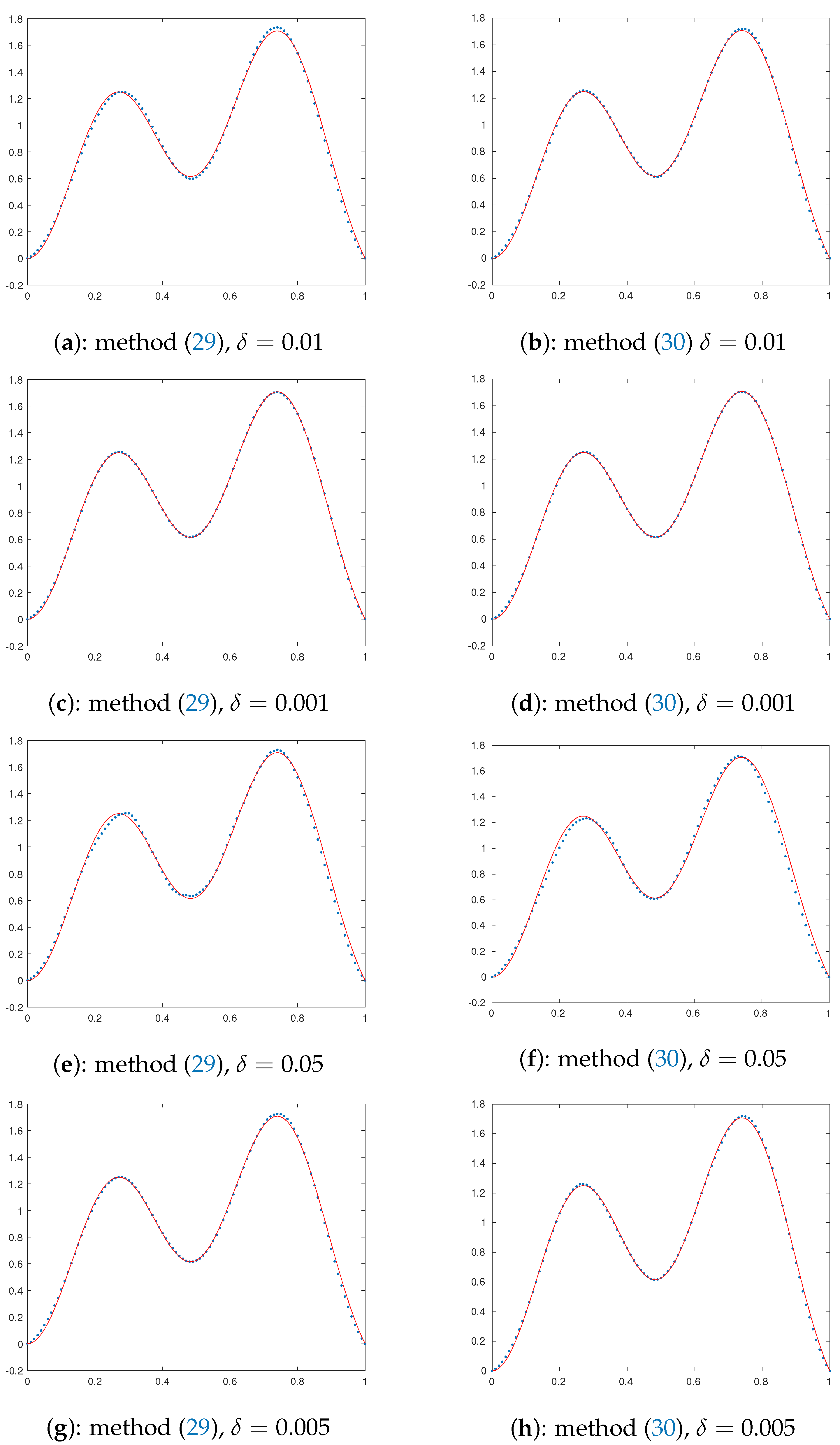
We have taken $c=4$ in (26) to compute $\alpha .$ Table 1 gives the values of $\delta ,$ the parameter $\alpha$ computed using (26), and the error $\parallel q_{k,\alpha }^{\delta }-\widehat{q}\parallel$ and time taken to compute $\alpha$ for different values of $\delta .$ The corresponding figures are provided in Figure 1.

Table 1. Computed $\alpha$ and computed error.

Method	$\mathit{\delta }$	$\mathit{\alpha }$	$\parallel {\mathit{q}}_{\mathit{k},\mathit{\alpha }}^{\mathit{\delta }}-\widehat{\mathit{q}}\parallel$	Elapsed Time in Seconds
	0.01	3.8147 × 10−6	0.0255	0.1664
	0.001	3.7253 × 10−9	0.0081	0.3884
(29)	0.05	3.0518 × 10−5	0.0298	0.1277
	0.005	9.5367 × 10−7	0.0178	0.1865
	0.01	1.9073 × 10−6	0.0138	0.2190
	0.001	3.7253 × 10−9	0.0086	0.5289
(30)	0.05	6.1035 × 10−5	0.0404	0.3383
	0.005	4.7684 × 10−7	0.0143	0.3988

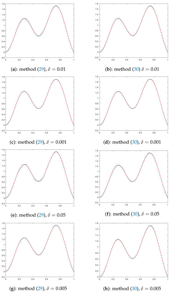
Figure 1. Exact ($----$) and computed solutions ($\ast \ast \ast$) for various parameters given against each subfigure.

We compare our method with that of the most widely used iterative method [26] for (5), which is the regularized Gauss Newton method, in which the iterations $x_{\alpha ,k}^{\delta }$ are defined for $k=0,1,2,\dots$ by

$$f_{k+1,{\alpha }_{k+1}}^{\delta }=f_{k,{\alpha }_k}^{\delta }-{({\mathcal{L}}^{\prime }{\left(f_{k,{\alpha }_k}^{\delta }\right)}^{*}{\mathcal{L}}^{\prime }\left(f_{k,{\alpha }_k}^{\delta }\right)+{\alpha }_{k}I)}^{-1}[{\mathcal{L}}^{\prime }{\left(f_{k,{\alpha }_k}^{\delta }\right)}^{*}(\mathcal{L}\left(f_{k,{\alpha }_k}^{\delta }\right)-y^{\delta })+\alpha (f_{k,{\alpha }_k}^{\delta }-f_0)],$$

(30)

where $f_{0,\alpha }^{\delta }:=x_0.$ Here, $\left({\alpha }_k\right)$ is a given sequence of numbers such that

$${\alpha }_k>0,1<\frac{{\alpha }_k}{{\alpha }_{k+1}}\le r\mathrm{and}\underset{k\to \infty }{lim}{\alpha }_k=0$$

for some constant $r>1.$

Stopping index: Choose $k_{\delta }$ as the first positive integer that satisfies

$$\frac{1}{2}(\parallel F\left(x_{k_{\delta }}^{\delta }\right)-y^{\delta }\parallel +\parallel F\left(x_{k_{\delta }-1}^{\delta }\right)-y^{\delta }\parallel \le \tau \delta ,$$

(31)

where $\tau >1$ is a sufficiently large constant not depending on $\delta .$ We have taken $\lambda =1.05$ and ${\alpha }_k=1/k$ in our computations.

We use a 4-core 64 bit Windows machine with 11th Gen Intel(R) Core(TM) i5-1135G7 CPU @ 2.40GHz for all our computations (using MATLAB).

Clearly, the table shows that our approach requires less computational time than that of method (30).

5. Conclusions

We introduced a new SC and a new PCS for the TR of nonlinear ill-posed problems. Our PCS does not require knowledge of $\nu$, and it gives the error estimate

$$\parallel f_{\alpha }^{\delta }-\widehat{f}\parallel =\left\{\begin{array}{c}O\left({\delta }^{\frac{2\nu }{2\nu +1}}\right),0<\nu \le \frac{1}{2}\\ O\left({\delta }^{\frac{1}{2}}\right),\nu >\frac{1}{2}\end{array}\right..$$

The advantage of our method is that one can compute the RP $\alpha$ before computing the regularized solution $f_{\alpha }^{\delta }.$ We also applied the method to the parameter identification problem modeled as in Example 1 and obtained favourable numerical results.

References

- Hadamard, J. Lectures on Cauchy’s Problem in Linear Partial Differential Equations; Dover Publications: New York, NY, USA, 1953. [Google Scholar]
- Ramm, A.G. Inverse Problems: Mathematical and Analytical Techniques with Applications to Engineering; Springer: New York, NY, USA, 2004. [Google Scholar]
- Akimova, E.N.; Misilov, V.E.; Sultanov, M.A. Regularized gradient algorithms for solving the nonlinear gravimetry problem for the multilayered medium. Math. Methods Appl. Sci. 2020, 21, 7012. [Google Scholar] [CrossRef]
- Byzov, D.; Martyshko, P. Three-Dimensional Modeling and Inversion of Gravity Data Based on Topography: Urals Case Study. Mathematics 2024, 12, 837. [Google Scholar] [CrossRef]
- Scherzer, O.; Engl, H.W.; Kunisch, K. Optimal a posteriori parameter choice for Tikhonov regularization for solving nonlinear ill-posed problems. SIAM. J. Numer. Anal. 1993, 30, 1796–1838. [Google Scholar] [CrossRef]
- Engl, H.W.; Hanke, M.; Neubauer, A. Regularization of Inverse Problems; Kluwer Academic Publisher: Dordrecht, The Netherlands; Boston, MA, USA; London, UK, 1996. [Google Scholar]
- Flemming, J. Generalized Tikhonov Regularization and Modern Convergence Rate Theory in Banach Spaces; Shaker Verlag: Aachen, Germany, 2012. [Google Scholar]
- Mair, B.A. Tikhonov regularization for finitely and infinitely smoothing operators. SIAM J. Math. Anal. 1994, 25, 135–147. [Google Scholar] [CrossRef]
- Engl, H.W.; Kunisch, K.; Neubauer, A. Convergence rates for Tikhonov regularization of nonlinear ill-posed problems. Inverse Probl. 1989, 5, 523–540. [Google Scholar] [CrossRef]
- Jin, Q.N.; Hou, Z.Y. On the choice of regularization parameter for ordinary and iterated Tikhnov regularization of nonlinear ill-posed problems. Inverse Probl. 1997, 13, 815–827. [Google Scholar] [CrossRef]
- Jin, Q.N.; Hou, Z.Y. On an a posteriori parameter choice strategy for Tikhnov regularization of nonlinear ill-posed problems. Numer. Math. 1999, 83, 139–159. [Google Scholar]
- Rieder, A. On the regularization of nonlinear ill-posed problems via inexact Newton iterations. Inverse Probl. 1999, 15, 309–327. [Google Scholar] [CrossRef]
- Vasin, V.; George, S. Expanding the applicability of Tikhonov’s regularization and iterative approximation for ill-posed problems. J. Inverse -Ill-Posed Probl. 2014, 22, 593–607. [Google Scholar] [CrossRef]
- Blaschke, B. Some Newton Type Methods for the Regularization of Nonlinear Ill-posed Problems. Trauner 1996, 13, 729. [Google Scholar]
- Nair, M.T. Linear Operator Equations: Approximation and Regularization; World Scientific: Singapore, 2009. [Google Scholar]
- Argyros, I.K.; George, S.; Jidesh, P. Inverse free iterative methods for nonlinear ill-posed operator equations. Int. J. Math. Math. Sci. 2014, 2014, 754154. [Google Scholar] [CrossRef]
- George, S. On conversence of regularized modified Newton’s method for nonlinear ill-posed problems. J. Inv. Ill-Posed Probl. 2010, 18, 133–146. [Google Scholar] [CrossRef]
- George, S.; Nair, M.T. An a posteriori parameter choice for simplified regularization of ill-posed problems. Inter. Equat. Oper. Th. 1993, 16, 392–399. [Google Scholar] [CrossRef]
- Hohage, T. Logarithmic convergence rates of the iteratively regularized Gauß-Newton method for an inverse potential and an inverse scattering problem. Inverse Probl. 1997, 13, 1279–1299. [Google Scholar] [CrossRef]
- Mahale, P.; Singh, A.; Kumar, A. Error estimates for the simplified iteratively regularized Gauss-Newton method under a general source condition. J. Anal. 2022, 31, 295–328. [Google Scholar] [CrossRef]
- Chen, D.; Yousept, I. Variational source condition for ill-posed backward nonlinear Maxwell’s equations. Inverse Probl. 2019, 35, 025001. [Google Scholar] [CrossRef]
- Hohage, T.; Weidling, F. Verification of a variational source condition for acoustic inverse medium scattering problems. Inverse Probl. 2015, 31, 075006. [Google Scholar] [CrossRef]
- Hohage, T.; Weidling, F. Variational source condition and stability estimates for inverse electromagnetic medium scattering problems. Inverse Probl. 2017, 11, 203–220. [Google Scholar]
- Hohage, T.; Weidling, F. Characerizations of variational source conditions, converse results, and maxisets of spectral regularization methods. SIAM J. Numer. Anal. 2017, 55, 598–620. [Google Scholar] [CrossRef]
- Hofmann, B.; Kaltenbacher, B.; Póschl, C.; Scherzer, O. A convergence rates result for Tikhonov regularization in Banach spaces with non-smooth operators. Inverse Probl. 2007, 23, 987–1010. [Google Scholar] [CrossRef]
- Jin, Q. On the iteratively regularized Gauss-Newton method for solving nonlinear ill-posed problems. Math. Comput. 2000, 69, 1603–1623. [Google Scholar]
- Jin, Q. A convergence analysis of the iteratively regularized Gauss-Newton method under Lipschitz condition. Inverse Probl. 2008, 24, 045002. [Google Scholar] [CrossRef]
- Mahale, P.; Dixit, S.K. Convergence analysis of simplified iteratively regularized Gauss-Newton method in a Banach space setting. Appl. Anal. 2017, 97, 1386785. [Google Scholar] [CrossRef]
- Bakushinskii, A. The problem of the convergence of the iterativley regularized Gauß-Newton method. Comput. Maths. Math. Phys. 1992, 32, 1353–1359. [Google Scholar]
- Bakushinskii, A. Iterative methods without saturation for solving degenerate nonlinear operator equations. Dokl. Akad. Nauk. 1995, 1, 7–8. [Google Scholar]
- Bakushinskii, A.; Kokurin, M. Iterative Methods for Approximate Solution of Inverse Problems; Springer: Berlin/Heidelberg, Germany, 2004. [Google Scholar]
- Blaschke, B.; Neubauer, A.; Scherzer, O. On convergence rates for the iteratively regularized Gauß-Newton method. Ima J. Numer. Anal. 1997, 17, 421–436. [Google Scholar] [CrossRef]
- Deuflhard, P.; Engl, H.W.; Scherzer, O. A convergence analysis of iterative methods for the solution of nonlinear ill-posed problems under affinely invariant conditions. Inverse Probl. 1998, 14, 1081–1106. [Google Scholar] [CrossRef]
- Hanke, M. Regularizing properties of a truncated Newton-CG algorithm for nonlinear inverse problems. Numer. Funct. Anal. Optim. 1997, 18, 971–993. [Google Scholar] [CrossRef]
- Kaltenbacher, B. A posteriori parameter choice strategies for some Newton type methods for the regularization of nonlinear ill-posed problems. Numer. Math. 1998, 79, 501–528. [Google Scholar] [CrossRef]
- Mahale, P. Simplified Generalized Gauss-Newton iterative method under Morozove type stopping rule. Numer. Funct. Anal. Optim. 2015, 36, 1448–1470. [Google Scholar] [CrossRef]
- Krasnoselskii, M.A.; Zabreiko, P.P.; Pustylnik, E.I.; Sobolevskii, P.E. Integral Operators in Spaces of Summable Functions; Noordhoff International Publ.: Leyden, IL, USA, 1976. [Google Scholar]
- Ford, W. Numerical Linear Algebra with Applications; Academic Press: New York, NY, USA, 2015; pp. 163–179. [Google Scholar]
Disclaimer/Publisher’s Note: The statements, opinions and data contained in all publications are solely those of the individual author(s) and contributor(s) and not of MDPI and/or the editor(s). MDPI and/or the editor(s) disclaim responsibility for any injury to people or property resulting from any ideas, methods, instructions or products referred to in the content. |
© 2024 by the authors. Licensee MDPI, Basel, Switzerland. This article is an open access article distributed under the terms and conditions of the Creative Commons Attribution (CC BY) license (https://creativecommons.org/licenses/by/4.0/).