Numerical Analysis of Flow Structure Evolution during Scour Hole Development: A Case Study of a Pile-Supported Pier with Partially Buried Pile Cap

Abstract

This study numerically investigates a pile-supported pier, which comprises a column with a partially buried pile cap and a group of piles, recognizing that partially buried pile caps lead to the highest scour depth. Most research has focused on equilibrium scour conditions in laboratory settings, overlooking the detailed dynamics of horseshoe vortices around pile groups. This study aims to clarify the flow structure and vortex dynamics at a pile-supported pier during local scour hole development stages using an in-house developed numerical model. The model’s accuracy is validated against flat-channel and compound pier reference cases. For the pile-supported pier, fixed bed geometry was used in flow simulations at selected scouring stages. Results show significant changes in flow structure and vortex formation with scour hole time development, particularly as the bed surface moves away from the pile cap. The study reveals variations in vortex size, number, and positioning, alongside turbulent kinetic energy and Reynolds shear stress distributions over time. High positive Reynolds shear stress near the bed during intermediate scouring stages highlights the complex interactions within the flow field. This research provides the first detailed visualization of flow structure evolution within a scour hole at a pile-supported pier.

1. Introduction

Scouring around bridge piers is an important subject in fluvial hydraulics. Local pier scouring manifests as a complex phenomenon arising from complex interactions among flow dynamics, the pier structure, and sediment bed characteristics. Overall, the primary scour activity mainly occurs in the frontal zone of the pier [1] and the main flow feature upstream of the pier is usually marked by a system of horseshoe vortices, “shed quasi-periodically” [2]. For a single-pier case, the approaching flow is diverted vertically by the pier. Subsequently, the downward flow in front of the pier deflects at the bed and interacts with the incoming flow, forming a rotational flow system recognized as the horseshoe vortex (HV) system. This mechanism leads to the detachment of the approaching boundary layer from the bed surface, culminating in the formation of the HV system upstream of the pier. For a fixed flat-bed condition, Roulund et al. [3] indicated that the position of the separation point is primarily influenced by the roughness of the bed, the pier Reynolds number (Re_D), and the ratio of the thickness of the approach boundary layer to the diameter of the pier. For a scoured bed condition, the position of the separation point is at the upstream edge of the local scour hole, where the slope of the bed changes. Consequently, the HV system is formed inside the scour hole.

In general, the HV system includes a main (large) vortex accompanied by several smaller secondary vortices, all surrounding the base of the pier and extending downstream for several pier diameters until losing their identity [3]. Dargahi [2] conducted experimental investigations into the flow structure at a vertically mounted circular pier on a fixed flat bed and observed that the number of vortices forming upstream of the pier is dependent on Re_D. Kirkil et al. [4] conducted numerical simulations of the HV system around a single circular pier at the equilibrium scour-hole condition. The corresponding calculations, at Re_D = 16,000, presented four necklace vortices upstream of the pier in the time-averaged flow. A large and stable vortex associated with a small (but very coherent) neighboring vortex was predicted at the pier’s base. Moreover, two secondary vortices were predicted upstream of the large vortex inside the scour hole. Guan et al. [5] experimentally investigated the characterization of the HV system at a time developing a clear-water scour hole around a single circular pier at Re_D = 13,680. The results indicated the evolution of the HV system from an initial small vortex to three vortices, consisting of one large vortex and two smaller vortices. Furthermore, approximately 24 h after the onset of the scour process, the main vortex’s position asymptotically approached stability. It is worth noting that the experimental test duration to reach quasi-equilibrium scour-hole conditions mentioned above was 48 h.

Concerning the vortex size, for example, Muzzammil and Gangadhariah [6] conducted experimental investigations into the time-averaged characteristics of the HV system during the scouring process around a circular pier. Their measurements revealed that the shape of the main HV is elliptical within the vertical symmetry plane. In accordance, Muzzammil and Gangadhariah [6] evaluated the vortex size based on the mean diameter of the corresponding ellipse. The results indicate that the size of the main vortex is about 0.2 times the pier diameter (0.2D) at the fixed flat-bed condition for Re_D ranging from 10⁴ to 1.4 × 10⁵, with the main vortex size exhibiting a linear increase with scour depth. Guan et al. [5] and Okhravi et al. [7] have similarly demonstrated that the size of the main vortex increases with the enlargement of the scour hole. Foregoing HV size, numerical investigations of Helmi and Shehata [8] have elucidated a correlation between the mean size of the main HV and scour depth throughout the evolution of the scour hole.

Kirkil et al. [4] showed that the main HV causes a significant increase in the shear stress values around the base of the pier. Generally, it is recognized that the scour occurs when the local bed shear stress exceeds a critical threshold. Using computational modeling, Kirkil et al. [4] calculated the time-averaged bed friction velocity values around a circular pier for the equilibrium scour-hole bathymetry. The corresponding indicated that the higher values of the bed friction velocity were predicted beneath the main HV and across most regions near the junction zone of the pier and the scoured bed. However, the predicted higher values are smaller than the local critical values, which aligns with the equilibrium scour-hole condition.

The pier geometry also influences the HV system. For example, Dey and Raikar [9] observed that the size of the main HV in front of a circular pier (with diameter D) is smaller than that of a square pier (with side length D) at the equilibrium scour-hole condition.

Overall, numerous research endeavors have focused on studying flow characteristics, specifically the HV system around individual bridge piers. However, in practical applications, modern bridges are typically built on foundations with complex geometries, such as pile-supported piers comprising columns and pile caps supported by groups of piles. This design choice is influenced by geotechnical and economic considerations. Consequently, some studies have explored the flow field around a pile-supported pier, mostly under fixed flat-bed conditions. Beheshti and Ataie-Ashtiani [10] conducted an experimental investigation of the flow field around a pile-supported pier with the flat-bed condition. In addition, Beheshti and Ataie-Ashtiani [11] examined how scour holes affect the turbulent flow field around a pile-supported pier, focusing mainly on areas outside the scour hole zone. Gautam et al. [12] experimentally investigated flow and turbulence characteristics around simple and complex piers on a flat rigid bed surface. Alemi et al. [13] characterized turbulent flow around a pile-supported pier with a flat bed using wall-modeled large-eddy simulation and the immersed boundary method.

In contrast to single piers, the local scour hole time evolution for pile-supported piers unfolds through different stages linked to the gradual exposure of the pier elements in the local scour evolution [14]. In accordance, when the pile cap is partially buried in the bed, a complex scouring process occurs around the pier. Experimental studies by Moreno et al. [14] indicate that the above-referred pile cap position potentially maximizes scour depth under equilibrium conditions compared to the situations where the pile cap is completely above or below the initial bed level.

The present study aims to utilize the developed numerical model of the authors (as detailed in [15,16]) to investigate the flow structure, notably the detailed horseshoe vortices, around a pile-supported pier at intermediate stages and equilibrium conditions of local scour holes. To the best of the authors’ knowledge, studies into the temporal evolution of the HV system around a pile-supported pier with a scoured bed have not been published. For the present simulations, the detailed bathymetry of the local scour holes was obtained from the experimental study of Ramos et al. [17] concerning the scour hole time development around a pile-supported pier (available at https://www.fe.up.pt/numpiers, accessed on 28 July 2024). At each stage of the local scour hole process selected for analysis, the corresponding bed geometry was considered fixed in the flow calculations to capture the details of the flow structure. Overall, this study scrutinizes vortice formation inside scour holes for a critical situation of a partially buried pile cap in the initial bed configuration, aiming to provide further cautious design improvements.

In the next section, the governing equations and numerical approach are summarized. In Section 3, the results of two validation test cases are presented. Section 4 describes the model setup for the pile-supported pier and the corresponding numerical results are presented and discussed in Section 5. Finally, the main conclusions are summarized in Section 6.

2. Numerical Model

The governing equations consist of the space-filtered Navier–Stokes and continuity equations commonly referred to as large-eddy simulation (LES), which are formulated as follows:

$${\displaystyle \frac{\mathsf{\partial }{u}_i}{\mathsf{\partial }t}}=-{\displaystyle \frac{1}{V_F}}\left(u_j{A}_j{\displaystyle \frac{\mathsf{\partial }{u}_i}{\mathsf{\partial }{x}_j}}\right)-{\displaystyle \frac{1}{\rho }}{\displaystyle \frac{\mathsf{\partial }\varnothing }{\mathsf{\partial }{x}_i}}+{\displaystyle \frac{{W\tau }_i}{\rho V_F}}+{\displaystyle \frac{1}{V_F}}{\displaystyle \frac{\mathsf{\partial }\left( \left(\nu +{\nu }_t\right) A_j {\tau }_{ij}\right)}{\mathsf{\partial }{x}_j}}$$

(1)

$${\displaystyle \frac{\mathsf{\partial }}{\mathsf{\partial }{x}_i}}\left(u_i{A}_i\right)=0$$

(2)

where $x_i$’s are the Cartesian coordinates and $u_i$’s are the corresponding filtered velocity components. t represents time, $\rho$ denotes the fluid density and $\varnothing$ refers to pseudo-pressure. The kinematic viscosity is denoted by ν, and ${\nu }_t$ represents the eddy viscosity. Moreover, the term ${W\tau }_i$ represents the wall shear stresses and ${\tau }_{ij}$ is the strain rate tensor.

A comprehensive account of the numerical model is provided by Alemi et al. [16] and Alemi [15]. In essence, the governing equations are solved on a Cartesian grid system. To incorporate the effects of pier and bed geometry into the governing equations, the geometry is transformed into fractional areas ($A_i$) and volumes ($V_F$) within each grid cell. Moreover, the numerical model uses a wall function that estimates instantaneous wall shear stresses, thereby reducing computational cost in comparison to a fully resolved LES. Also, the employed wall function accommodates the bed roughness effect in the calculations. Finally, the numerical model uses the Smagorinsky subgrid-scale model to estimate the turbulent eddy viscosity.

The fractional step method is used to solve the governing equations as follows:

$${\displaystyle \frac{{u_i}^{*}-{u_i}^n}{∆t}}={\displaystyle \frac{3}{2}} \mathrm{M}\left({u_i}^n\right)-{\displaystyle \frac{1}{2}}\mathrm{M}\left({u_i}^{n-1}\right)-{\displaystyle \frac{1}{\rho }}{\displaystyle \frac{\mathsf{\partial }{\varnothing }^n}{\mathsf{\partial }{x}_i}}$$

(3)

$${\displaystyle \frac{{u_i}^{**}-{u_i}^{*}}{∆t}}={\displaystyle \frac{1}{\rho }}{\displaystyle \frac{\mathsf{\partial }{\varnothing }^n}{\mathsf{\partial }{x}_i}}$$

(4)

$${\displaystyle \frac{\mathsf{\partial }}{\mathsf{\partial }{x}_i}}\left(A_i{\displaystyle \frac{\mathsf{\partial }{\varnothing }^{n+1}}{\mathsf{\partial }{x}_i}}\right)={\displaystyle \frac{\rho }{∆t}}{\displaystyle \frac{\mathsf{\partial }\left(A_i{u_i}^{**}\right)}{\mathsf{\partial }{x}_i}}$$

(5)

$${\displaystyle \frac{{u_i}^{n+1}-{u_i}^{**}}{∆t}}=-{\displaystyle \frac{1}{\rho }}{\displaystyle \frac{\mathsf{\partial }{\varnothing }^{n+1}}{\mathsf{\partial }{x}_i}}$$

(6)

where ${u_i}^{*}$ and ${u_i}^{**}$ are intermediate velocities. $∆t$ represents the time step size and the superscript n denotes the time step counter. The operator M stands for the convection, wall shear stress and viscous terms of Equation (1).

The numerical model employs the explicit Adams–Bashforth scheme for time integration. Spatial terms are approximated using the central difference scheme, except for the convection terms. In turbulent channel flow simulation, the convection terms are approximated using the central difference scheme, while in bridge pier flow simulation, the QUICK scheme is utilized for stability reasons. It is worth noting that a turbulent channel flow simulation provides realistic inflow conditions for the flow simulation at a bridge pier.

When periodic boundary conditions are applied in the streamwise direction, such as in a channel flow simulation, a mean pressure gradient driving the flow in that direction is included as a source term in the Navier–Stokes equation for the corresponding calculations:

$${\mathrm{S}}^{n+1}={\mathrm{S}}^n+{\displaystyle \frac{\alpha }{∆t}}\left(V_{\mathrm{t}\mathrm{a}\mathrm{r}\mathrm{g}\mathrm{e}\mathrm{t}}+V^{n-1}-2 V^n\right)$$

(7)

where S represents the source term, which remains constant in space but may vary over time. The parameter V denotes the average cross-sectional flow velocity, and $\alpha$ is a dimensionless coefficient.

3. Validation Test Cases

For the present study, the numerical model is evaluated through two validation cases: (i) a fully developed channel flow, characterized by turbulent flow between two parallel planes, driven by a constant pressure gradient, and (ii) a turbulent flow around a compound pier with the scoured bed.

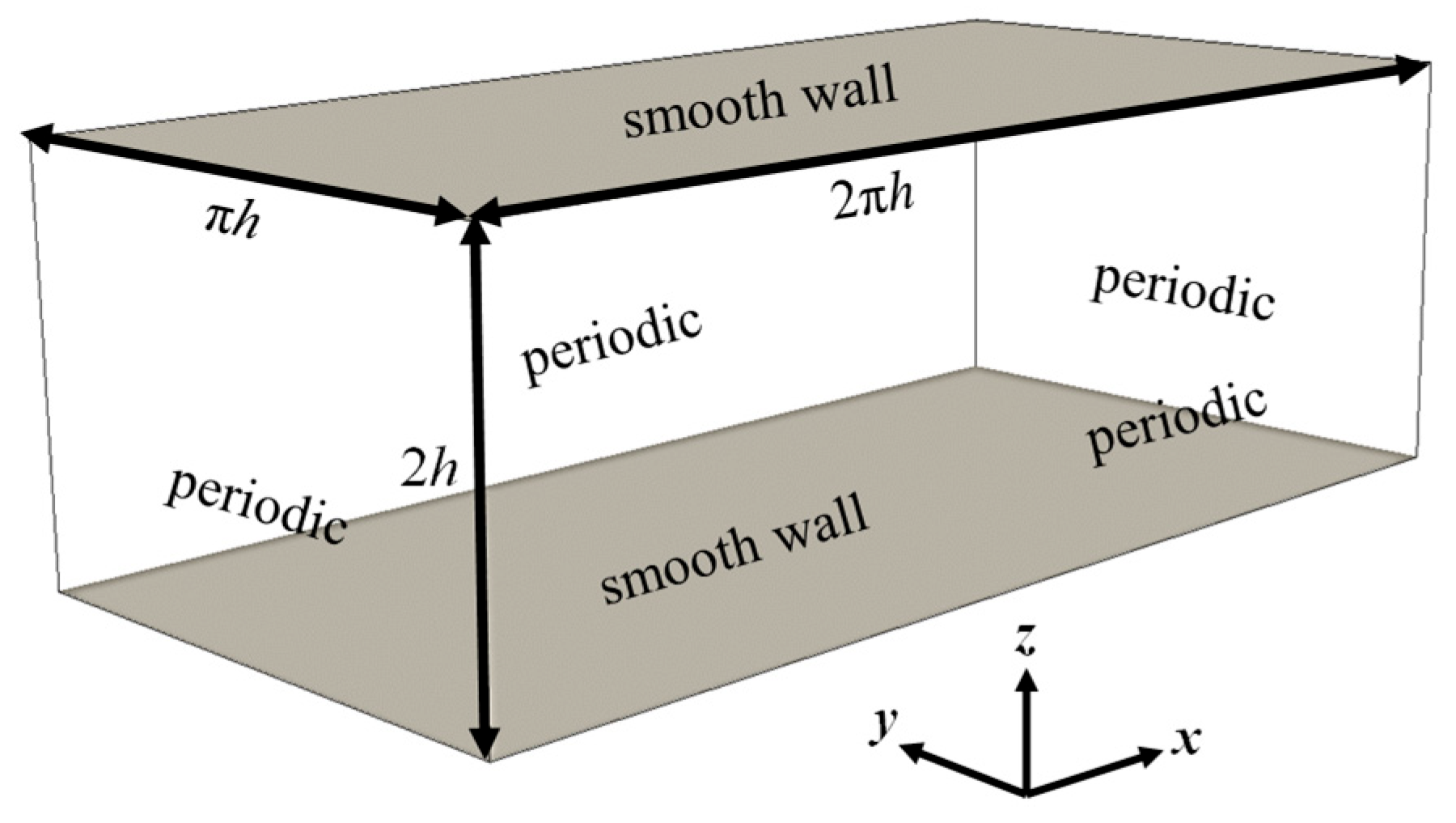
3.1. Turbulent Channel Flow

The LES calculations were performed for a flat-channel flow at a Reynolds number of ${\mathrm{R}\mathrm{e}}_h=Uh/\nu$ = 10,935, where $U$ is the velocity and $h$ represents the channel half-height. According to Hinterberger et al. [18], the above-referred Reynolds number corresponds to the friction Reynolds number of ${\mathrm{R}\mathrm{e}}_{\tau }=u_{*}h/\nu =590$, where $u_{*}$ is the friction velocity. Consequently, the present LES results are compared with those reported by Moser et al. [19], obtained using the Direct Numerical Simulation (DNS) method for ${\mathrm{R}\mathrm{e}}_{\tau }=590$. To evaluate the present LES Smagorinsky model, the wall function was not used only for this specific validation (fully resolved LES calculations). It is noteworthy to mention that the DNS method directly uses the Navier–Stokes equations.

The computational domain dimensions (2πh × πh × 2h) and boundary conditions (illustrated in Figure 1) align with those utilized in the referenced DNS study. Stationary smooth walls were situated at the bottom (z = −h) and top (z = h) of the domain, while periodic boundary conditions were applied in the longitudinal (x) and transverse (y) directions. Uniform grid spacing was considered in the x and y directions. In the vertical direction z, grid cell height was minimized near the wall surfaces to ensure that three consecutive grid points in the wall-normal direction reside within the viscous sub-layer. In accordance, a wall damping function was exclusively applied for this case to make sure that the eddy viscosity is reduced near the wall surfaces. In total, 120 grid cells were utilized for each direction.

The corresponding profiles of the normalized mean u velocity (longitudinal velocity component), root-mean-square values of the velocity components fluctuations ($\sqrt{\overline{u^{\mathrm{’}}{u}^{\mathrm{’}}}}$, $\sqrt{\overline{v^{\mathrm{’}}{v}^{\mathrm{’}}}}$ and $\sqrt{\overline{w^{\mathrm{’}}{w}^{\mathrm{’}}}}$), and the xz component of the Reynolds stress tensor ($\overline{u^{\mathrm{’}}{w}^{\mathrm{’}}}$) are presented in Figure 2. The overbar and angle brackets in Figure 2 denote, respectively, time and spatial (longitudinal and transverse directions) averaging. Overall, the LES results obtained are consistent with the DNS findings. Minor discrepancies observed in certain regions can be attributed to the fact that in the DNS method and all turbulent scales are resolved temporally and spatially, whereas in the LES calculations, only the large-scale motions of the turbulent flow (large eddies) are directly computed, and the small-scale motions are modeled using a subgrid-scale model.

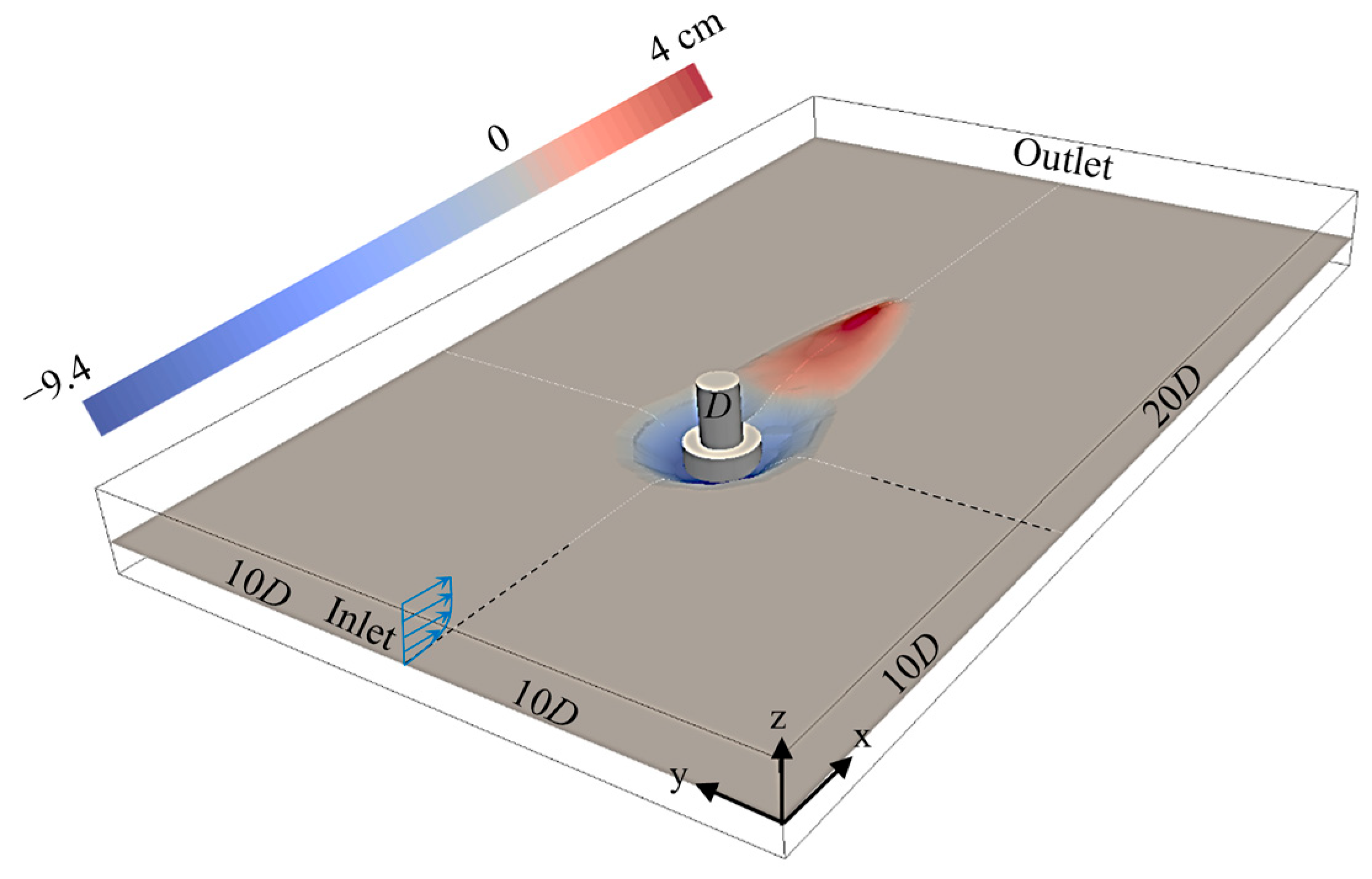
3.2. Compound Pier Flow

The simulation of the flow around a compound pier with a scour hole, illustrated in Figure 3, replicated the pier geometry and flow conditions from the experiment conducted by Kumar and Kothyari [20]. The pier model was a circular pier with a diameter of 0.114 m, supported by a circular foundation with a diameter of 0.21 m. The top surface of the foundation was positioned at z = −2.1 cm (z = 0 represents the channel bed level). The mean flow depth $h$ and the approach flow velocity $U_{\infty }$ were set at 0.16 m and 0.28 m/s, respectively.

A non-uniform grid system, with 313 × 254 × 85 (about 6.8 × 10⁶) grid cells, was used for the present LES calculations. The grid resolution is finer in the pier zone compared to the outer zone. The bed geometry model, associated with the scour hole developed 7 h after the beginning of the scouring process, was generated using the bed contour lines obtained from the experimental study [20]. For the numerical calculations, the bed level at each grid point between the available contour lines was predicted using linear interpolation from the nearest available data points.

The time-averaged horseshoe vortices at the vertical symmetry plane are shown in Figure 4. The present numerical simulation captures more detailed aspects of the HV system compared to the experimental measurements. Based on the numerical results, the downflow in front of the pier foundation is diverted upstream and downstream at the bottom of the scour hole, resulting in the formation of a strong and large vortex V2 together with a small junction vortex V1. In addition, two counter-rotating vortices (V3 and V4) were predicted upstream of V2 inside the scour hole. The flow structure predicted in front of the circular pier foundation closely resembles that obtained numerically by Kirkil et al. [4] for a single circular pier. Concerning the strong vortex V2, the corresponding maximum reverse flow velocity (negative $\overline{u}$ velocity) was predicted to be −0.53$U_{\infty }$ (equivalent to −0.15 m/s), a value that is similar to the one experimentally measured by Guan et al. [5] for a circular pier with a scoured bed.

In a comprehensive analysis, $\overline{u}$ velocity profiles were extracted at various positions on the symmetry plane and compared with the corresponding experimental data, as shown in Figure 5. Overall, the numerical results align well with the reference results. However, at x = 0.14 m, a discrepancy is noted in a region near the bed where the negative $\overline{u}$ velocity values were obtained numerically, while positive values were reported by Kumar and Kothyari [20]. In fact, at the above-referred zone, the longitudinal extent of the reverse flow area obtained numerically was slightly larger than that observed in the experimental study. Nevertheless, at x = 0.14 m (and x = 0.25 m), the time-averaged vertical velocity ($\overline{w}$) and root-mean-square velocity component fluctuations were accurately predicted across the flow depth, as shown in Figure 6.

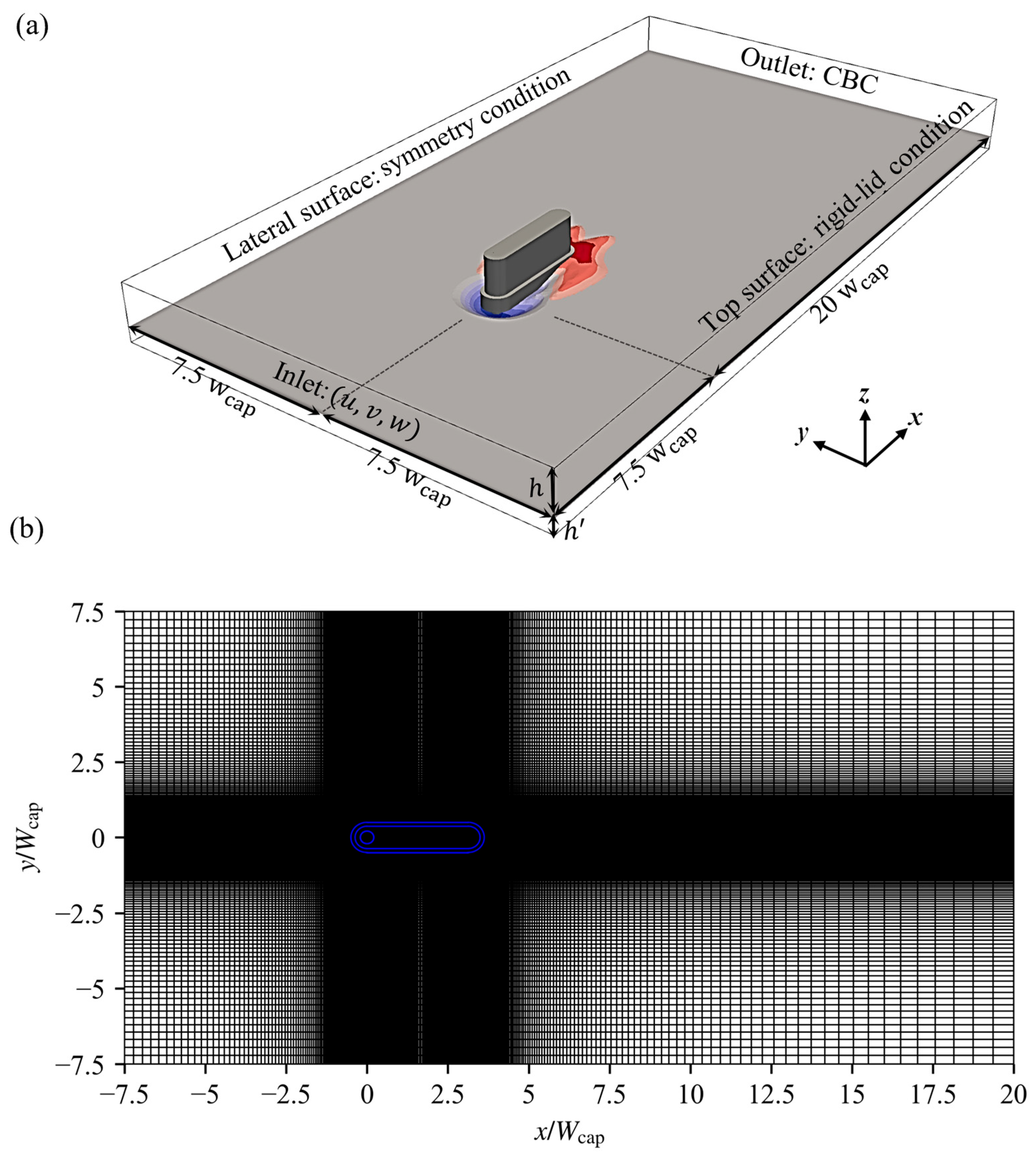
4. Model Setup for the Pile-Supported Pier Case

To investigate the temporal evolution of the flow field (mainly, the horseshoe vortices) around the pile-supported pier, numerical calculations were conducted at three distinct stages of the local scouring process: two intermediate stages (t = 1 and 12 h) and the equilibrium stage (t = 11 days) for the same experimental flow conditions of Ramos et al. [17]. The flow depth $h$ was set at 0.18 m, and the mean approach flow velocity $U_{\infty }$ is 0.327 m/s. The pier configuration consisted of a rectangular round-nose column and pile cap, supported by a column of four in-lined piles (forming a group of 1 × 4 piles). In this configuration, half of the pile-cap height ($0.5 {\mathrm{H}}_{\mathrm{c}\mathrm{a}\mathrm{p}}=2.9 \mathrm{c}\mathrm{m}$) protruded above the initial bed level. The geometric details of the pier are illustrated in Figure 7.

For the numerical simulations, the computational domain dimensions were 27.5 ${\mathrm{W}}_{\mathrm{c}\mathrm{a}\mathrm{p}}$ × 15 ${\mathrm{W}}_{\mathrm{c}\mathrm{a}\mathrm{p}}$ × (h + $h^{\prime }$) in longitudinal (x), transverse (y) and vertical directions (z), respectively. As shown in Figure 7, ${\mathrm{W}}_{\mathrm{c}\mathrm{a}\mathrm{p}}$ represents the pile cap width. The domain depth (h + $h^{\prime }$) includes the mean flow depth and the maximum local scour depth. Therefore, the vertical length $h^{\prime }$ (i.e., bed layer depth) was predefined at each numerical test by considering the corresponding scour depth obtained from the referenced experimental study. The pier was positioned in the symmetry plane of the domain at ${7.5 \mathrm{W}}_{\mathrm{c}\mathrm{a}\mathrm{p}}$ downstream from the inlet boundary section. The inflow conditions (i.e., instantaneous velocity components) were obtained from a periodic open-channel flow with identical ${\mathrm{Re}}_{\mathrm{h}}=58860$. The top surface was modeled as a shear-free rigid lid taking into account the small Froude number for this case (Fr = 0.25). At the outlet section, boundary conditions were set with zero pressure and convective boundary conditions (CBC) for the velocity components. The above-referred computational domain configuration is exemplified in Figure 8a, corresponding to the numerical test for the t = 1 h bed configuration.

The time step size was approximately 0.0015 s in all simulations, and the flow characteristics were collected over about 60 s (40,000 time steps) after the initial condition effects were eliminated from the calculations. For each numerical simulation, the corresponding bed geometry was obtained from the experimental study and considered as a fixed boundary (i.e., no sediment transport modeling).

The used grid configurations consisted of approximately 5.9 million cells (408 × 249 × 58) for the numerical test corresponding to t = 1 h, 7 million cells (408 × 249 × 69) for t = 12 h, and 11.6 million cells (501 × 249 × 93) for t = 11 days. The grid resolution is higher near the pier elements and bed surface, gradually becoming coarser further away from the pier and bed, as illustrated in Figure 8b. The grid-cell size increased spatially with an expansion ratio of approximately 1.03, ensuring that the grid presented a high spatial resolution in regions where vortices are expected to form. The quality of the grids is assessed using the method outlined by Pope [21], which stipulates that the unresolved portion of energy at each grid cell should not exceed 0.2. According to Figure 9, the unresolved turbulent kinetic energy is less than 0.2 in the majority of grid cells (84–93% of active cells), indicating that the turbulence was adequately resolved at most parts of the computational domain.

5. Results and Discussion

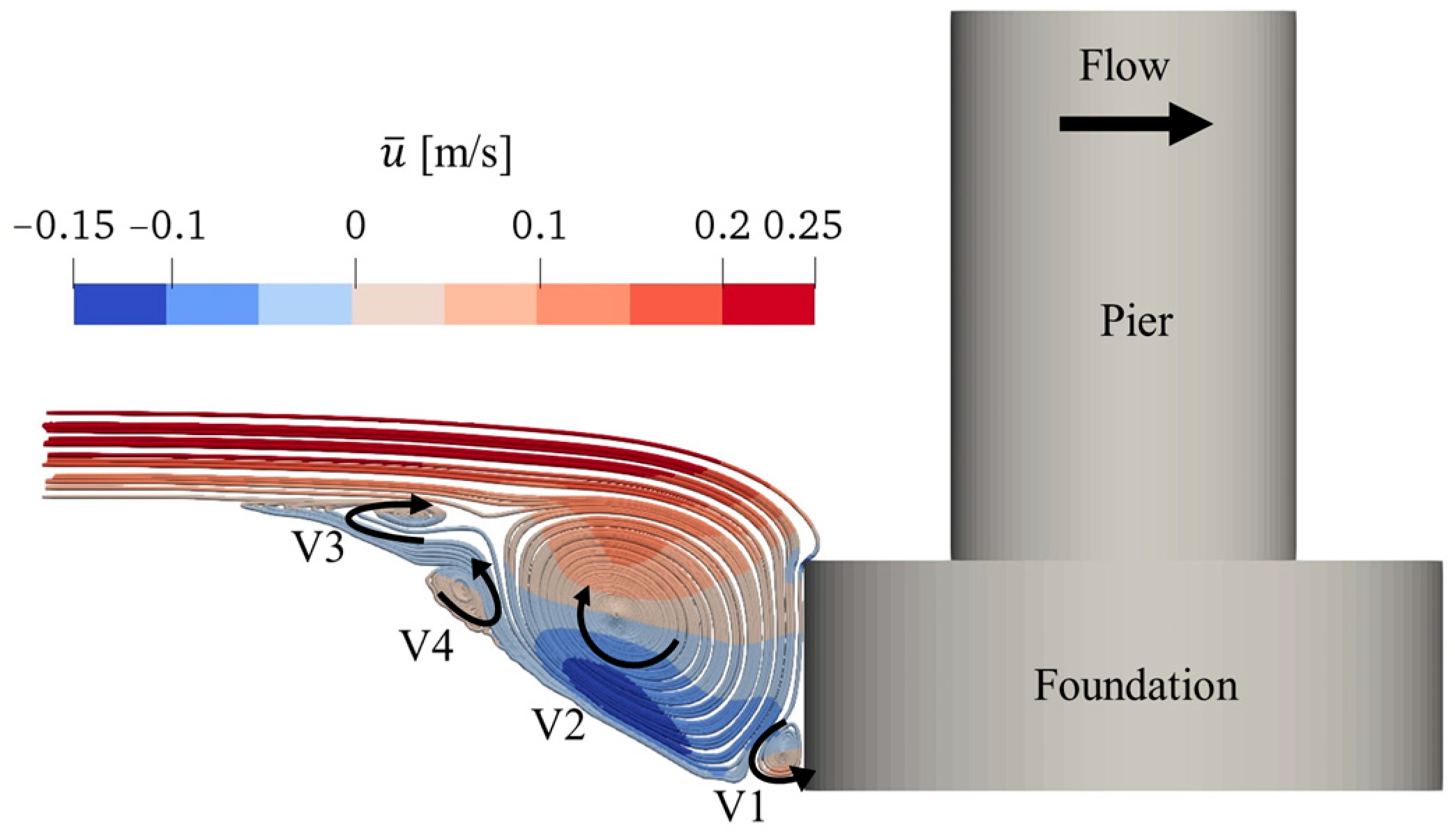
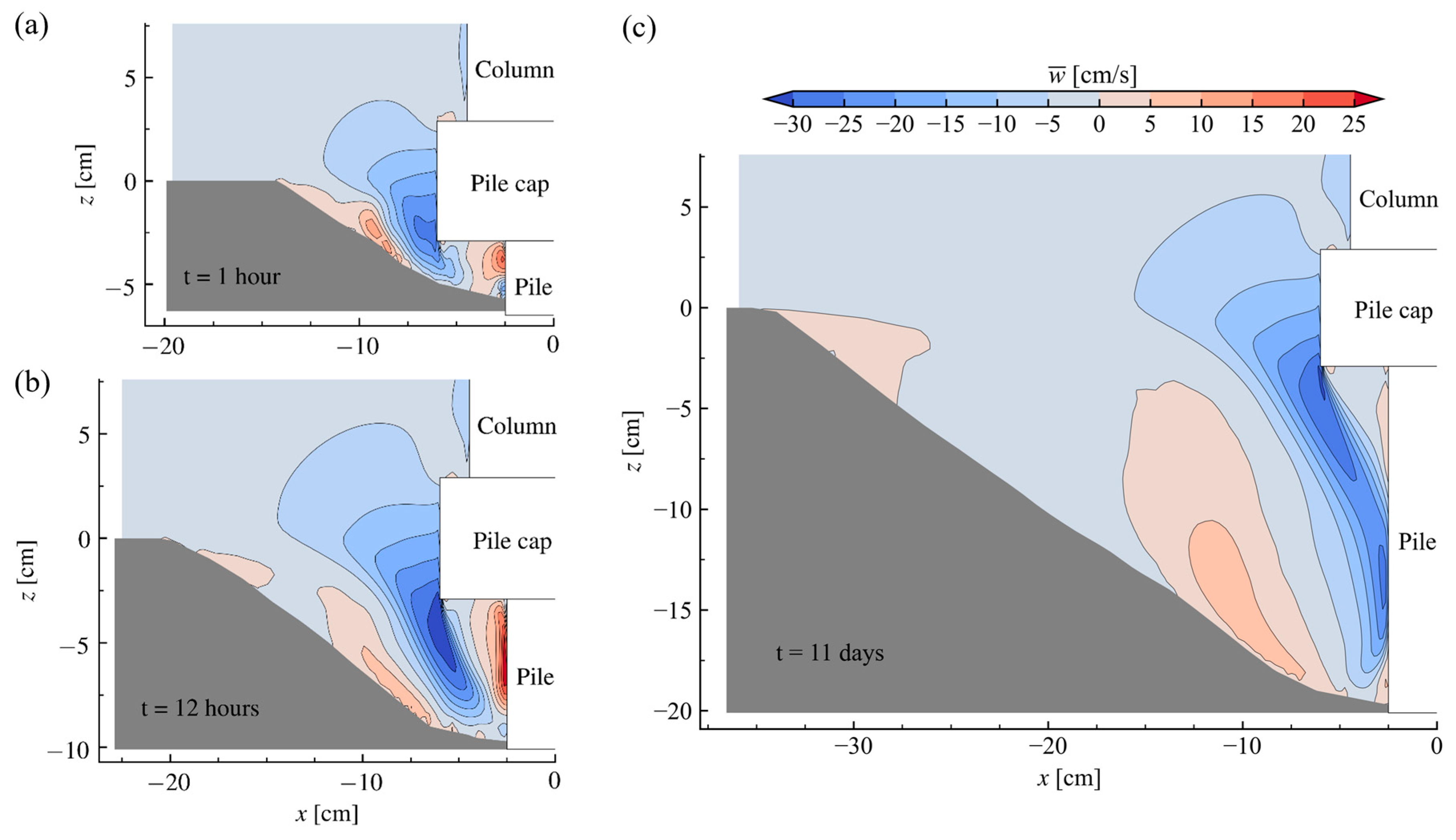
5.1. Flow Velocities and Streamline Patterns

A sequence of the time-averaged $u$ and $w$ velocities, along with the corresponding streamlines topology in front of the pier (at the vertical symmetry plane y = 0) is shown in Figure 10 and Figure 11 for the bed geometries corresponding to t = 1, 12 h, and 11 days. Given that the primary objective of this study is to investigate the evolution of horseshoe vortices during various stages of the local scour development process, the downstream flow zone is not relevant to the scope of this study.

At the symmetry plane y = 0, the approaching flow is deflected vertically by the column. The corresponding downward flow accelerates towards the pile cap, and the accelerated flow area expands over with the development of the local scour hole (as shown in Figure 11). The downflow is then deflected by the pile cap against the direction of the approaching flow, creating a small vortex on the upper face of the pile cap (highlighted in Figure 10). In front of the pile cap, at y = 0, the numerical results indicate that the flow turns downward, in which the corresponding maximum downflow occurs at a point close to the lower upstream edge of the pile cap (below the initial bed level of the channel) in all three stages of local scouring (refer to Figure 11).

The flow beneath the pile cap is also accelerated and then vertically deflected by the upstream pile. The corresponding upward flow is stronger than the downward flow at t = 1 h and 12 h (Figure 11a,b), but at t = 11 days, the downward flow is the stronger one (Figure 11c). This disparity is attributed to the gap between the pile cap and the scoured bed surface in front of the upstream pile, and consequently to the deflection-point position on the front face of the upstream pile. Indeed, for the intermediate stages of the local scouring process, the deflection point on the front face of the upstream pile takes place near the scoured bed surface, limiting the greater acceleration of the downward flow.

The vertically deflected flow in front of the upstream pile, at t = 1 and 12 h, is diverted backward by the scoured bed and pile cap, resulting in the formation of two vortices near the pile-bed junction (V1) and below the bottom face of the pile cap (V5), as shown in Figure 10a,b. At the equilibrium stage (t = 11 days), the accelerated flow beneath the pile cap is redirected by the mid-height of the upstream pile, and V5 has almost disappeared. Moreover, the corresponding junction vortex V1 rotates counter-clockwise, as shown in Figure 10c, which is contrary to the direction illustrated for the intermediate stages of the local scour hole process. It is noteworthy to note that changing the flow behavior directly in front of a pile-supported pier during the local scouring process can affect the corresponding sediment erosion rate compared to a single pier case.

The main horseshoe vortex (denoted by V2 in Figure 10) wraps around the pier and carries bed material away from it. At t = 1 h, V2 was completely formed upstream of the pile cap zone due to the small gap between the scoured bed surface and the pile cap. It subsequently progressed towards the upstream pile as the local scour hole developed over time. Notably, the main vortex V2 rotates clockwise for all studied scoured bed stages, consistent with findings reported for the compound pier case in Figure 4.

The obtained results also indicate that the approach flow separates at the upstream edge of the scour hole due to a change in the bed slope, resulting in the creation of a clockwise vortex, V3, immediately after this edge. At the equilibrium condition, the flow structure in that zone becomes slightly more complex with two small vortices, instead of one, rotating in the same direction as reported earlier. At t = 1 h, V3 is positioned directly upstream of the main vortex V2 within the scour hole. However, as the local scour hole develops over time, the vortices V2 and V3 become increasingly distant from each other, creating space for the formation of vortex V4 between them (attached to V2) but rotating in the opposite direction to the main vortex, V2.

Figure 12 presents the streamlines, obtained from the time-averaged v and w velocity components, at transverse cross-section x = 5 cm for different stages of the local scour hole development process. As shown in Figure 7, x = 5 cm lies between the first (upstream) and second piles to capture most of the vortices formed on the pier sides. It should be noted that notations of the vortices used for the presentation of the results at x = 5 cm differ from those discussed earlier in the longitudinal vertical plane y = 0.

According to Figure 12, different transverse flow patterns are observed when comparing the intermediate and equilibrium stages of the local scouring process. The streamline patterns at x = 5 cm indicate that the flow deflects sideways. However, at t = 11 days, the flow in the side zone of the scour hole tends to converge with the deflected flow (caused by the column), which is in agreement with the experimental observations of Beheshti and Ataie-Ashtiani [10,11] for a pile-supported pier.

Numerical simulations identified multiple vortices in the vicinity of the column, pile cap, and bed surface, with vortex size increasing in accordance with the scour depth. Specifics regarding the vortices and their respective locations are outlined below:

Above the channel-bed level, two vortices (labeled as 1 and 2, rotating in the same direction) are observed on the column and pile cap sides for all the bed geometries considered. Additionally, a vortex (3) forms near the bottom side edge of the pile cap at the selected intermediate stages but disappears at the equilibrium stage. By enlarging the scour hole, the pile cap side vortex (2) and a near-bed vortex (4) move apart, with vortex 4 relocating to the pile-group zone. Consequently, vortex 2 expands and covers most of the pile cap side face at t = 11 days. Vortex 4, along with vortices 5 and 6, facilitates the lift of sediment particles from the bed surface and transports them downstream, thereby contributing to the lateral widening of the scour hole. As depicted in Figure 12, vortex 6 emerges with the time development of the scour hole, which was not evident for the scour state corresponding to t = 1 h. Moreover, at t = 12 h, the scour hole has exposed the zone below the pile cap, where a small vortex (7) is formed due to flow contraction there. With the enlargement of the scour hole, at the equilibrium condition, vortex 7 vanishes, and almost the whole area beneath pile cap is swallowed up by the large vortex 4.

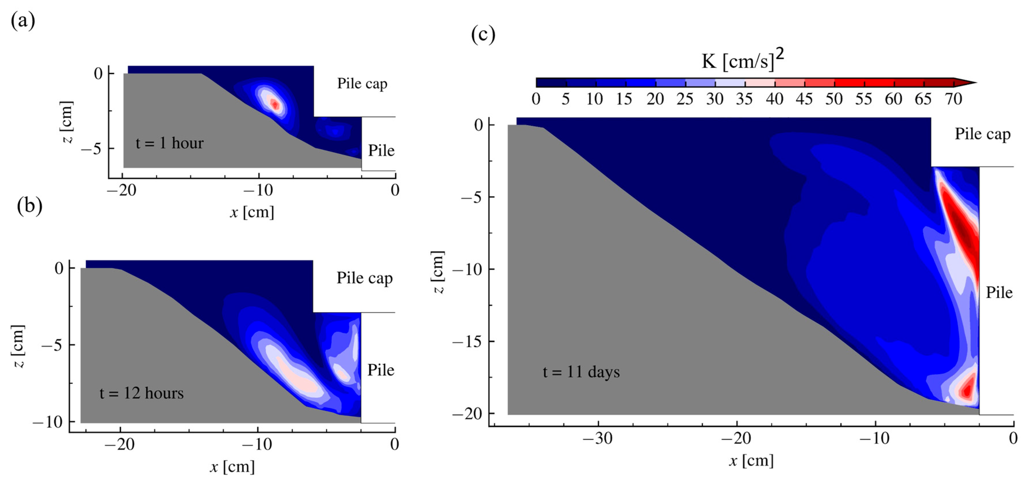
5.2. Turbulent Kinetic Energy

Figure 13 illustrates the distribution of Turbulent Kinetic Energy (TKE), denoted as K, at the vertical symmetry plane over the temporal evolution of the scour hole. Mathematically, TKE is defined as half of the sum of the mean-squares of velocity components fluctuations ($\mathrm{K}=0.5(\overline{u^{\prime }{u}^{\prime }}+\overline{v^{\prime }{v}^{\prime }}+\overline{w^{\prime }{w}^{\prime }}))$.

The numerical results show that the highest levels of turbulence energy are concentrated near the bed, decreasing as the scour depth develops over time. Referring to the velocity distribution shown in Figure 10, the elevated turbulence intensities align with the formation of the main vortex, V2, which significantly influences sediment particle uplift and scour hole extension. At the equilibrium stage, two distinct zones emerge near the upstream pile: one situated beneath the pile cap, and the other near the bottom of the scour hole. The former is attributed to the accelerated flow below the pile cap and the latter corresponds to the location of vortex V1 (Figure 10), thereby amplifying turbulence intensities.

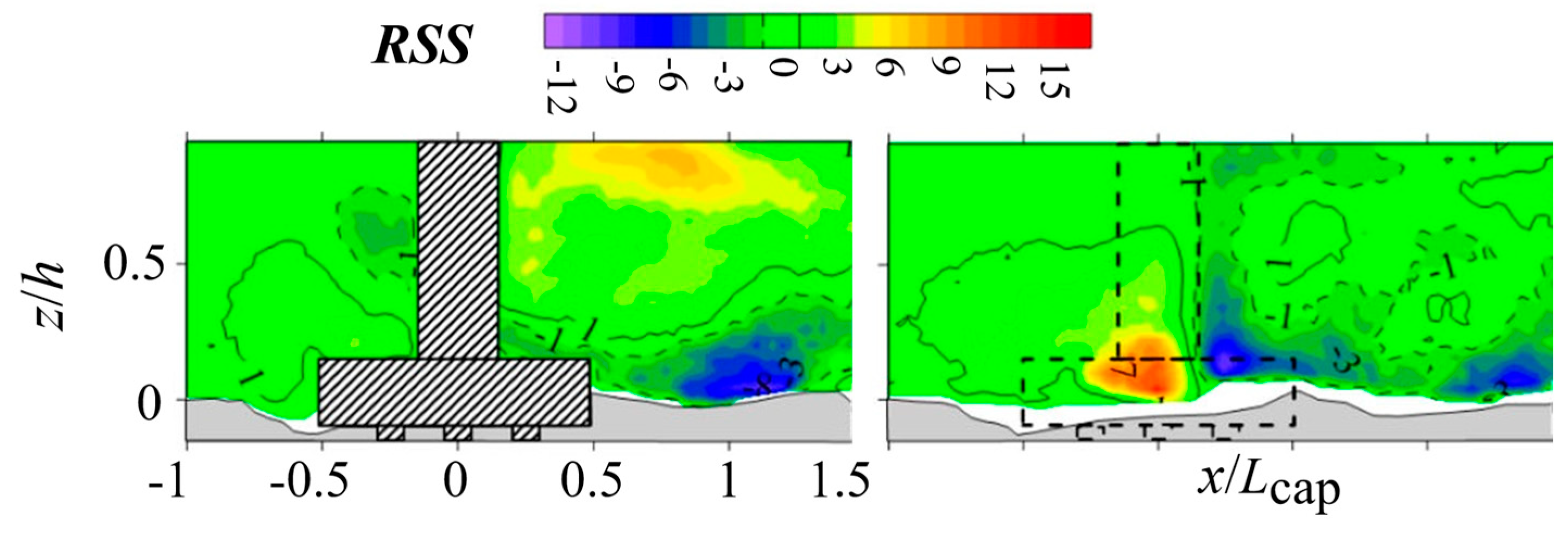
5.3. Reynolds Shear Stress

Figure 14 presents the temporal evolution of Reynolds shear stress (RSS), defined as $\mathrm{R}\mathrm{S}\mathrm{S}=-\rho \overline{u^{\prime }{w}^{\prime }}/{U_{\infty }}^2$. In the three representations of RSS contours corresponding to different time instances, negative RSS values (ranging between −4 and 0) have been computed in the front of the column. To facilitate comparison with the experimental findings of Gautam et al. [22], the RSS contours obtained by those authors under equilibrium conditions have been pictured in Figure 15. Their investigation revealed almost the same RSS magnitudes (ranging between −3 and 0) in this region along the vertical symmetry plane y = 0 (front of the column) as those found in the current study. Notably, Gautam et al. [22] focused also on characterizing RSS distribution downstream and lateral sides of the pier, which diverges from the scope of the present study.

According to the obtained results, as anticipated, regions exhibiting strong RSS values correspond closely with areas characterized by high values of K. Moreover, The observation is consistent with findings from the LES study by Kirkil and Constantinescu [23] and the experimental investigation by Guan et al. [5] concerning a single-pier under equilibrium conditions.

At t = 12 h, strong positive values of RSS near the bed are evident, amplifying the strength of the HV system and exacerbating scour extension by drifting sediment particles upstream of the scour hole. It is evident that RSS values may exceed those computed under equilibrium conditions (comparing t = 12 h and t = 11 days), attributed to heightened momentum exchange within this particular domain.

6. Conclusions

The comprehensive depiction of flow structure within the scour hole from various perspectives represents a novel contribution, particularly in the context of pile-supported piers, where prior studies offered limited insight into these outcomes.

In this study, an attempt was first made to validate a numerical model, developed under the research work of the authors, by considering two benchmark cases (namely, turbulent channel flow and compound pier flow). In summary, the corresponding numerical results, including the velocity components and turbulence intensities, align well with the reference data. This study then proceeded to investigate the flow structure around a pile-supported pier with a scoured bed. The pile-supported pier included a column and pile cap with round corners, supported by a row of four piles where half of the pile cap height was initially buried in the bed.

In summary, the obtained numerical results (time-averaged flow field) show that the flow pattern upstream of the pier considerably changes as the pile cap becomes more distant with time from the local scoured bed surface, possibly affecting the erosion rate in front of the pier. For example, directly in front of the upstream pile, the corresponding flow pattern is different at the time levels t = 1 h, 12 h and 11 days due to the interaction between the pile cap, bed surface and upstream pile. Further, at t = 1 h, the large and strong horseshoe vortex was completely formed upstream of the pile-cap position due to the small distance between the scoured-bed surface and pile cap; but it moved towards the upstream pile with time (i.e., increasing the scour depth). Moreover, upstream of the pier, the size and number of horseshoe vortices change with the time of development of the local scour hole.

This study also investigated the flow vortices at a vertical transverse plane (x = 5 cm). The corresponding numerical results indicate that the number and size of vortices increase by enlarging the scour hole. For example, at t = 12 h when the scour hole has uncovered the zone below the pile cap, a small flow rotation was predicted in the zone below the pile cap due to the interaction between the bed geometry and pile cap, which has disappeared at the equilibrium stage (t = 11 days) as the local bed surface becomes distant from the pile cap.

The region exhibiting the strongest turbulence intensity and Reynolds shear stress within the scour hole corresponds to the location of the main vortex and near the bed, where large turbulent eddies are most likely to occur. Additionally, at the equilibrium stage, high Reynolds shear stress values were observed in regions characterized by strong downflow and the presence of the junction vortex in front of the upstream pile. The turbulence findings from present LES simulations demonstrate satisfactory alignment with published results derived from experimental measurements and numerical simulations. Overall, monitoring the evolving trends in vertical position, size, and circulation strength in the flow field is important. Understanding these trends aids in the optimal design of scour countermeasures, as the size and shape of vortices directly influence the dimensions of armoring measures, such as riprap, around bridge piers.

References

1. Unger, J.; Hager, W.H. Down-Flow and Horseshoe Vortex Characteristics of Sediment Embedded Bridge Piers. Exp. Fluids 2007, 42, 1–19. [Google Scholar] [CrossRef]
2. Dargahi, B. The Turbulent Flow Field around a Circular Cylinder. Exp. Fluids 1989, 8, 1–12. [Google Scholar] [CrossRef]
3. Alemi, M.; Pêgo, J.P.; Maia, R. Numerical Investigation of the Flow Behavior around a Single Cylinder Using Large Eddy Simulation Model. Ocean. Eng. 2017, 145, 464–478. [Google Scholar] [CrossRef]
4. Kirkil, G.; Constantinescu, S.G.; Ettema, R. Coherent Structures in the Flow Field around a Circular Cylinder with Scour Hole. J. Hydraul. Eng. 2008, 134, 572–587. [Google Scholar] [CrossRef]
5. Guan, D.; Chiew, Y.-M.; Wei, M.; Hsieh, S.-C. Characterization of Horseshoe Vortex in a Developing Scour Hole at a Cylindrical Bridge Pier. Int. J. Sediment Res. 2019, 34, 118–124. [Google Scholar] [CrossRef]
6. Muzzammil, M.; Gangadhariah, T. The Mean Characteristics of Horseshoe Vortex at a Cylindrical Pier. J. Hydraul. Res. 2003, 41, 285–297. [Google Scholar] [CrossRef]
7. Okhravi, S.; Gohari, S.; Alemi, M.; Maia, R. Numerical Modeling of Local Scour of Non-Uniform Graded Sediment for Two Arrangements of Pile Groups. Int. J. Sediment Res. 2023, 38, 597–614. [Google Scholar] [CrossRef]
8. Helmi, A.M.; Shehata, A.H. Three-Dimensional Numerical Investigations of the Flow Pattern and Evolution of the Horseshoe Vortex at a Circular Pier during the Development of a Scour Hole. Appl. Sci. 2021, 11, 6898. [Google Scholar] [CrossRef]
9. Dey, S.; Raikar, R.V. Characteristics of Horseshoe Vortex in Developing Scour Holes at Piers. J. Hydraul. Eng. 2007, 133, 399–413. [Google Scholar] [CrossRef]
10. Beheshti, A.A.; Ataie-Ashtiani, B. Experimental Study of Three-Dimensional Flow Field around a Complex Bridge Pier. J. Eng. Mech. 2010, 136, 143–154. [Google Scholar] [CrossRef]
11. Beheshti, A.A.; Ataie-Ashtiani, B. Scour Hole Influence on Turbulent Flow Field around Complex Bridge Piers. Flow Turbulence Combust 2016, 97, 451–474. [Google Scholar] [CrossRef]
12. Gautam, P.; Eldho, T.I.; Mazumder, B.S.; Behera, M.R. Experimental Study of Flow and Turbulence Characteristics around Simple and Complex Piers Using PIV. Exp. Therm. Fluid Sci. 2019, 100, 193–206. [Google Scholar] [CrossRef]
13. Alemi, M.; Pêgo, J.P.; Maia, R. Characterization of the Turbulent Flow around Complex Geometries Using Wall-Modeled Large Eddy Simulation and Immersed Boundary Method. Int. J. Civ. Eng. 2020, 18, 279–291. [Google Scholar] [CrossRef]
14. Moreno, M.; Maia, R.; Couto, L. Effects of Relative Column Width and Pile-Cap Elevation on Local Scour Depth around Complex Piers. J. Hydraul. Eng. 2016, 142, 04015051. [Google Scholar] [CrossRef]
15. Alemi, M. Numerical Simulation of the Flow Behavior around Bridge Piers. Ph.D. Thesis, University of Porto, Porto, Portugal, 2018. Available online: https://repositorio-aberto.up.pt/bitstream/10216/117225/2/301519.pdf (accessed on 11 July 2024).
16. Alemi, M.; Pêgo, J.P.; Maia, R. Numerical Simulation of the Turbulent Flow around a Complex Bridge Pier on the Scoured Bed. Eur. J. Mech. B Fluids 2019, 76, 316–331. [Google Scholar] [CrossRef]
17. Ramos, P.X.; Bento, A.M.; Maia, R.; Pêgo, J.P. Characterization of the Scour Cavity Evolution around a Complex Bridge Pier. J. Appl. Water Eng. Res. 2016, 4, 128–137. [Google Scholar] [CrossRef]
18. Hinterberger, C.; Fröhlich, J.; Rodi, W. 2D and 3D Turbulent Fluctuations in Open Channel Flow with Re τ = 590 Studied by Large Eddy Simulation. Flow Turbul. Combust 2008, 80, 225–253. [Google Scholar] [CrossRef]
19. Moser, R.D.; Kim, J.; Mansour, N.N. Direct Numerical Simulation of Turbulent Channel Flow up to Reτ=590. Phys. Fluids 1999, 11, 943–945. [Google Scholar] [CrossRef]
20. Kumar, A.; Kothyari, U.C. Three-Dimensional Flow Characteristics within the Scour Hole around Circular Uniform and Compound Piers. J. Hydraul. Eng. 2012, 138, 420–429. [Google Scholar] [CrossRef]
21. Pope, S.B. Ten Questions Concerning the Large-Eddy Simulation of Turbulent Flows. New J. Phys. 2004, 6, 35. [Google Scholar] [CrossRef]
22. Gautam, P.; Eldho, T.I.; Behera, M.R. Effects of Pile-Cap Elevation on Scour and Turbulence around a Complex Bridge Pier. Int. J. River Basin Manag. 2023, 21, 283–297. [Google Scholar] [CrossRef]
23. Kirkil, G.; Constantinescu, G. Flow and Turbulence Structure around an In-stream Rectangular Cylinder with Scour Hole. Water Resour. Res. 2010, 46, 2010WR009336. [Google Scholar] [CrossRef]
Figure 1. Flat-channel case: computational domain with the corresponding dimensions and boundary conditions.
Modelling 05 00046 g001
Figure 2. Comparison of the present LES results with the corresponding DNS results [19] for the turbulent channel flow at R e τ = 590 (the flow quantities were averaged in space and over time).
Modelling 05 00046 g002
Figure 3. Compound pier case: bed geometry and computational domain dimensions.
Modelling 05 00046 g003
Figure 4. Time-averaged horseshoe vortices upstream of the compound pier, present study.
Modelling 05 00046 g004
Figure 5. Comparison of the present numerical results ( u ¯ velocity values [m/s]), solid lines, with the corresponding experimental results [20], scatters, at different positions x = −0.17, −0.14, −0.1, 0.14, 0.25 and 0.4 m (measured from the pier center), compound pier case.
Modelling 05 00046 g005
Figure 6. Comparison of the present numerical results ( w ¯ velocities and root-mean-square values of the velocity components fluctuations), solid lines, with the corresponding experimental results [20], scatters, at different positions (x = 0.14 and 0.25) downstream of the compound pier.
Modelling 05 00046 g006
Figure 7. Geometric characteristics of the pile-supported pier.
Modelling 05 00046 g007
Figure 8. Pile-supported pier case: computational domain and boundary conditions (a); and computational mesh in the horizontal plane (b) for the numerical test with bed geometry corresponding to t = 1 h (note that only the upstream pile interacts with the flow at t = 1 h).
Modelling 05 00046 g008
Figure 9. Percentage of the unresolved turbulent kinetic energy for all numerical tests corresponding to the pile-supported pier case.
Modelling 05 00046 g009
Figure 10. Time-averaged u velocities and streamlines at the vertical symmetry plane y = 0 (front of the pile-supported pier) for the bed geometries corresponding to (a) t = 1 h, (b) t = 12 h and (c) t = 11 days. The mean approach water depth is 18 cm.
Modelling 05 00046 g010
Figure 11. Time-averaged w velocities at the vertical symmetry plane y = 0 (front of the pile-supported pier) for the bed geometries corresponding to (a) t = 1 h, (b) t = 12 h and (c) t = 11 days. The mean approach water depth is 18 cm.
Modelling 05 00046 g011
Figure 12. Streamlines at the transverse cross-section x = 5 cm at: (a) t = 1 h, (b) t = 12 h and (c) t = 11 days (looking downstream); pile-supported pier case.
Modelling 05 00046 g012
Figure 13. Contours of the turbulent kinetic energy (K) at the vertical symmetry plane y = 0 (front of the pile-supported pier) for the bed geometries corresponding to (a) t = 1 h, (b) t = 12 h and (c) t = 11 days.
Modelling 05 00046 g013
Figure 14. Contours of the Reynolds shear stress (RSS) at the vertical symmetry plane y = 0 (front of the pile-supported pier) for the bed geometries corresponding to (a) t = 1 h, (b) t = 12 h and (c) t = 11 days.
Modelling 05 00046 g014
Figure 15. Contours of the Reynolds shear stress (RSS) at the vertical symmetry plane y = 0 (front of the pile-supported pier, left image) and side plane (right image) under equilibrium conditions for a scenario involving a partially buried pile cap in the study of Gautam et al. [22].
Modelling 05 00046 g015
Disclaimer/Publisher’s Note: The statements, opinions and data contained in all publications are solely those of the individual author(s) and contributor(s) and not of MDPI and/or the editor(s). MDPI and/or the editor(s) disclaim responsibility for any injury to people or property resulting from any ideas, methods, instructions or products referred to in the content.