
Numerical Simulation of Turbulent Fountains with Negative Buoyancy

 , ,
, , 
Abstract
:1. Introduction
2. Experiments
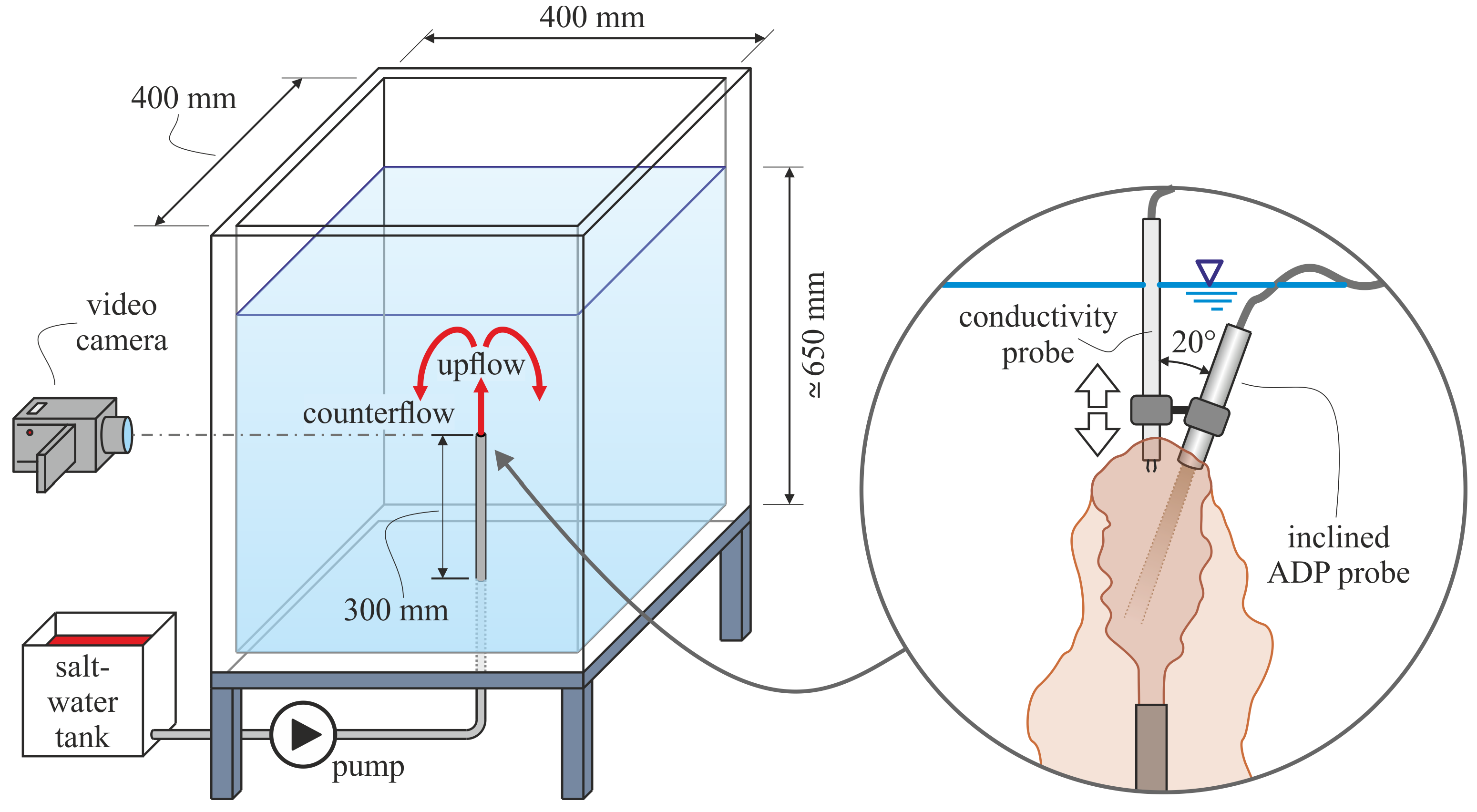
2.1. Apparatus
2.2. Data Recording
3. Numerical Model
3.1. Model Setup
3.2. Computational Domain, Boundary, and Initial Conditions
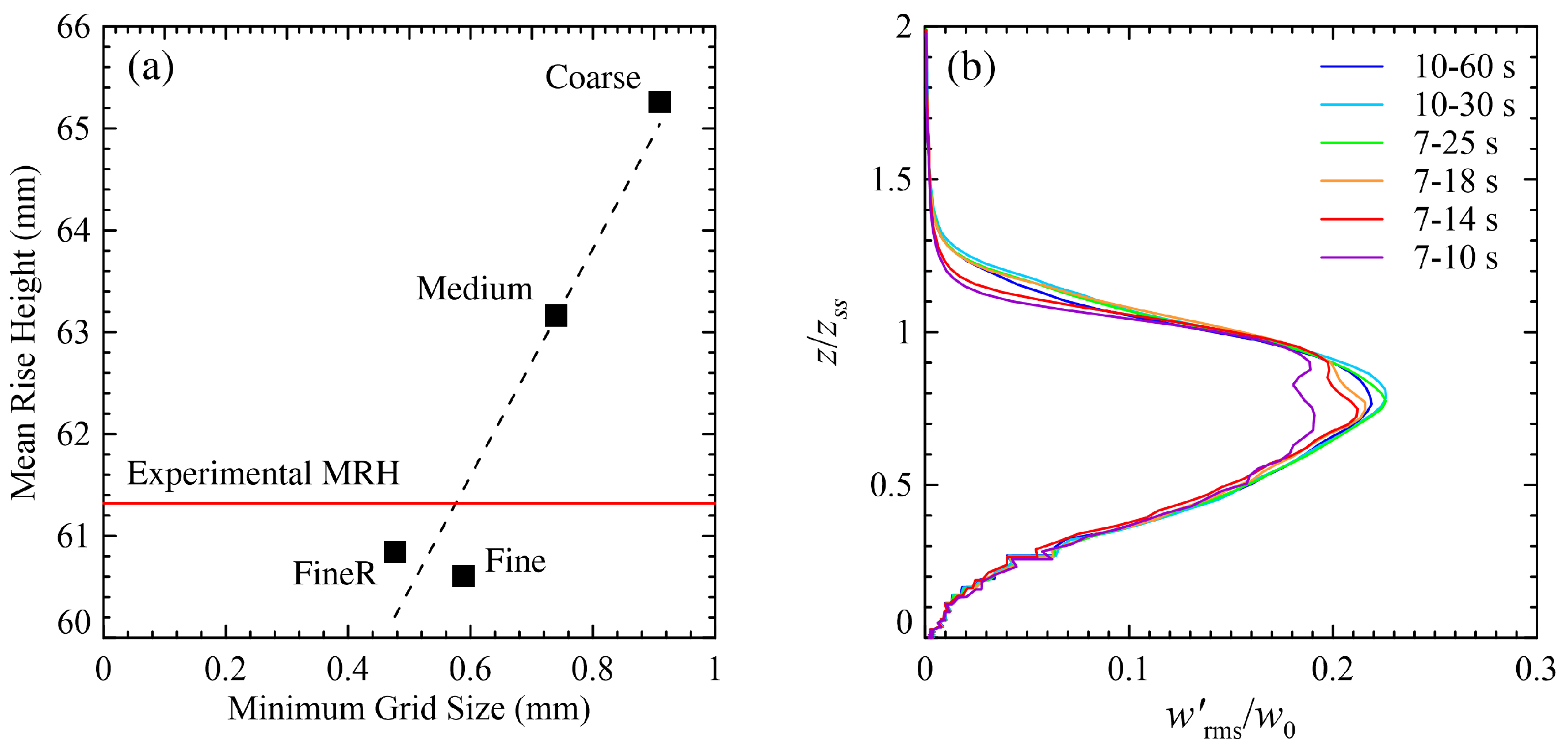
3.3. Mesh Sensitivity Analysis
4. Results
4.1. Fountain Statistics
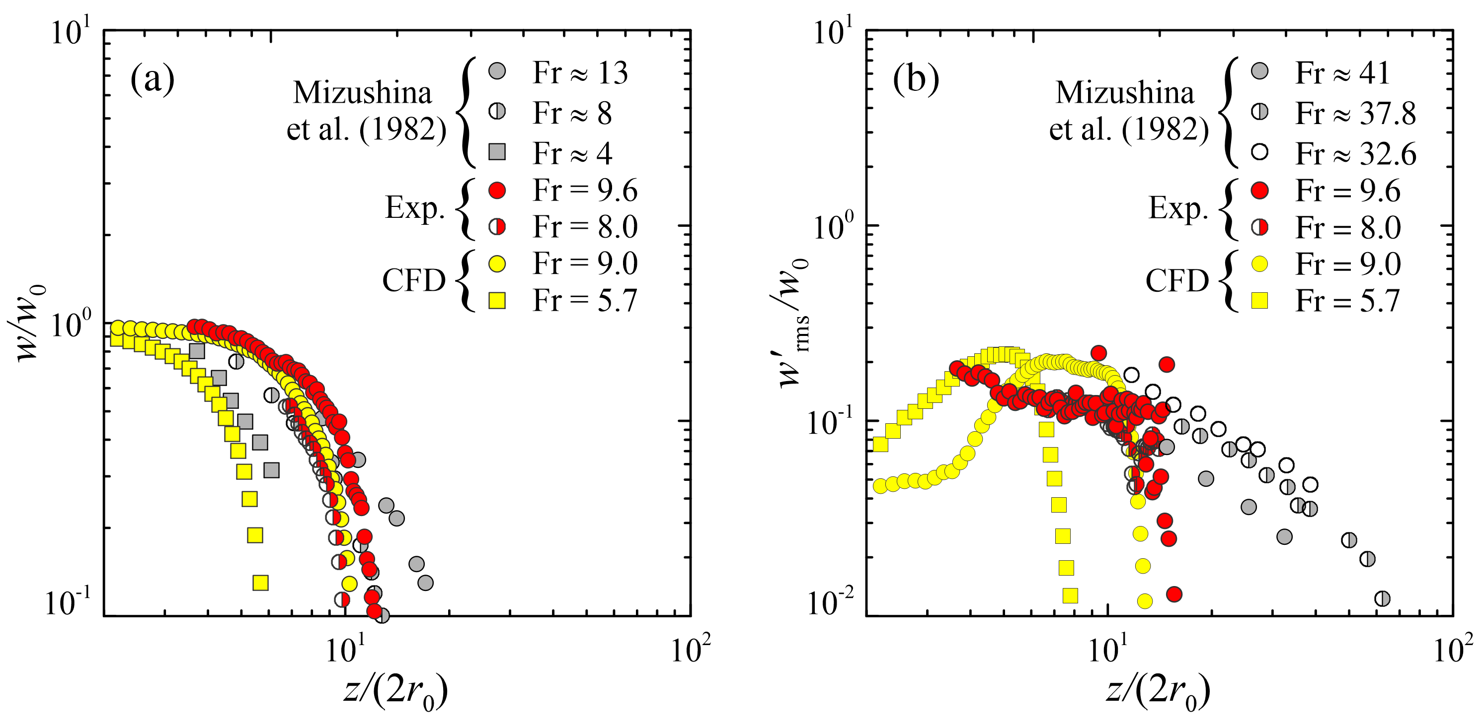
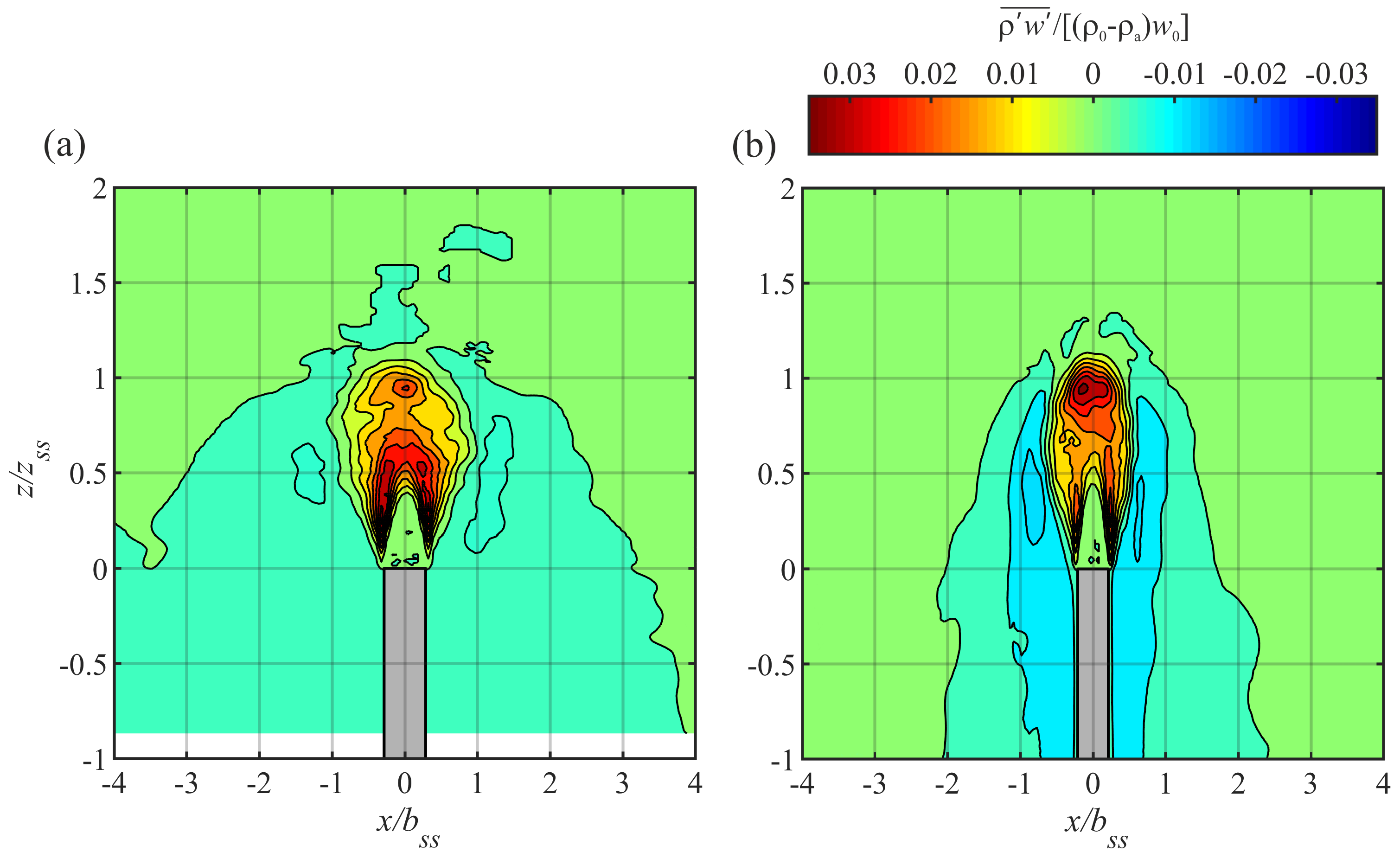
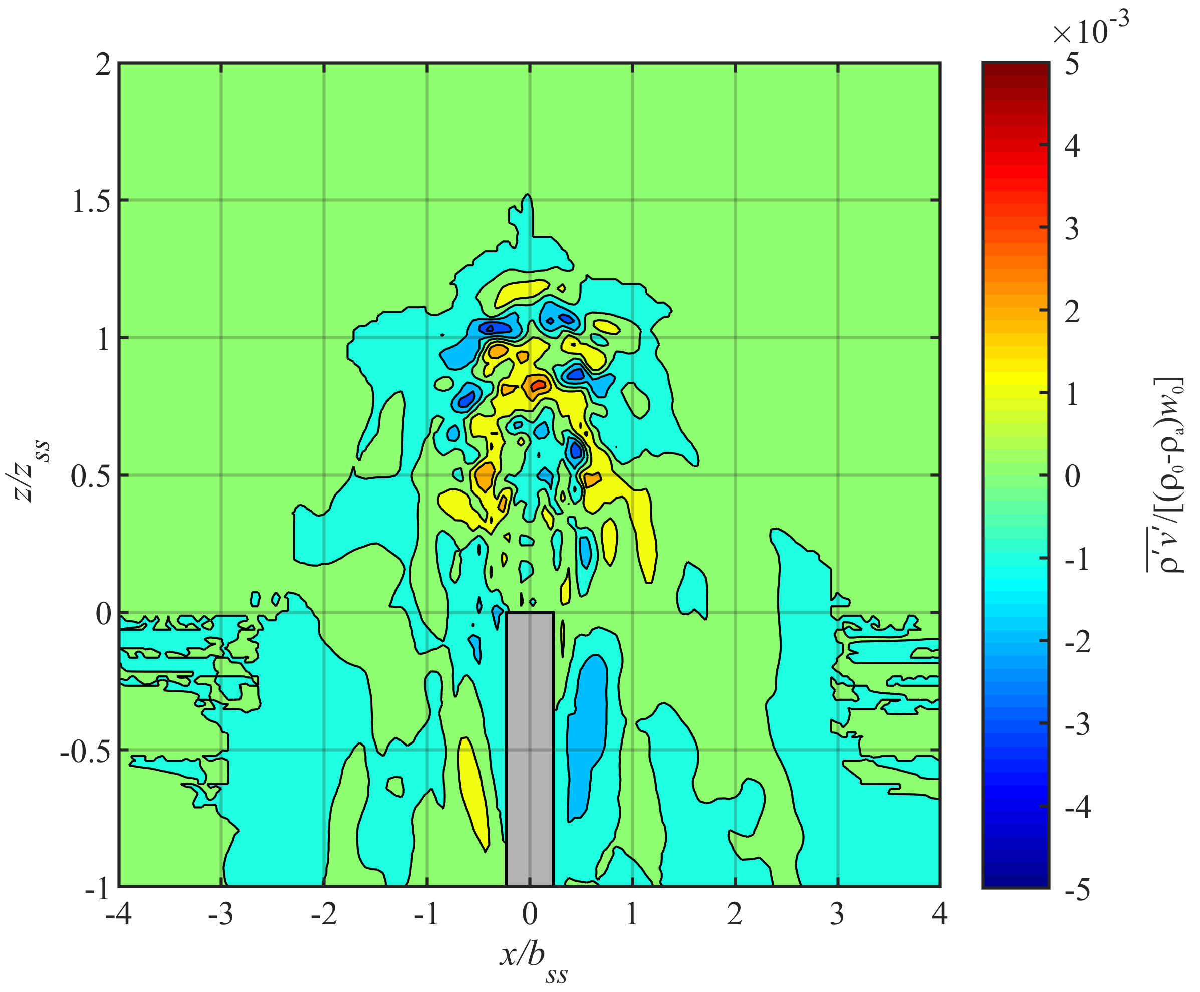
4.2. Mean Flow and Turbulence
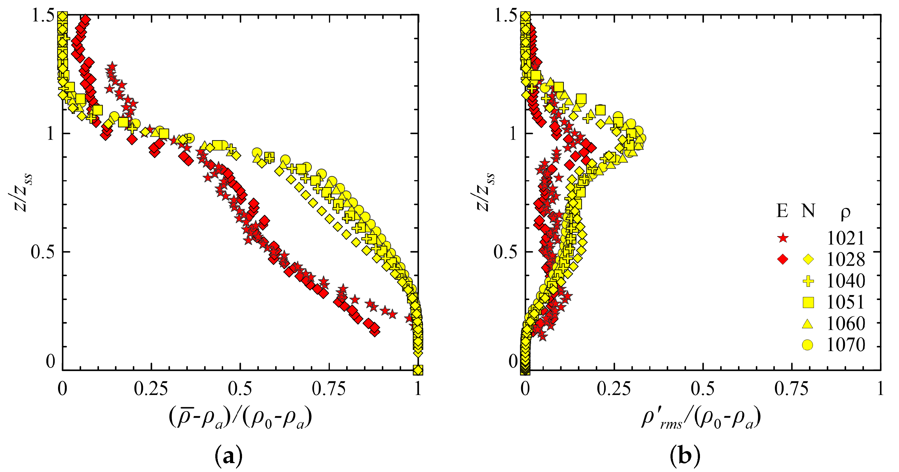
4.3. Density Profile and Mass Exchanges
4.4. Practical Applications
5. Conclusions
Author Contributions
Funding
Data Availability Statement
Acknowledgments
Conflicts of Interest
Nomenclature
| Fountain-top semi-width | |
| Outer diameter of the source | |
| Inner diameter of the source | |
| Source Froude number | |
| g | Gravitational acceleration |
| Buoyancy of the source fluid | |
| p | Order of convergence |
| Q | Discharge |
| r | Constant refinement ratio |
| Inner radius of the source | |
| Source Reynolds number | |
| w | Vertical velocity |
| Velocity of the fluid at the source | |
| RMS of the vertical velocity fluctuations | |
| z | Vertical axis |
| Peak height of the fountain | |
| Mean rise height of the fountain | |
| Mean peak height | |
| Mean trough height | |
| Phase fraction of the ambient fluid | |
| Phase fraction of the source fluid | |
| Density of the ambient fluid | |
| Density of the source fluid | |
| Standard deviation of the rise height | |
| ADP | Acoustic Doppler Profiler |
| CGI | Grid Convergence Index |
| CFD | Computational Fluid Dynamics |
| CFL | Courant–Friedrichs–Lewy |
| DNS | Direct Numerical Simulation |
| LES | Large Eddy Simulation |
| MRH | Mean Rise Height |
| RANS | Reynolds-Averaged Navier–Stokes |
| RMS | Root Mean Square |
| SGS | Sub-Grid Scale |
| U-RANS | Unsteady Reynolds-Averaged Navier–Stokes |
| VoF | Volume of Fluid |
Appendix A. Governing Equations
References
- Hunt, G.; Burridge, H. Fountains in industry and nature. Annu. Rev. Fluid Mech. 2015, 47, 195–220. [Google Scholar] [CrossRef]
- Hassanzadeh, H.; Taghavi, S.M. A review on free miscible buoyant jets. Phys. Fluids 2024, 36, 061301. [Google Scholar] [CrossRef]
- Baines, W.; Corriveau, A.; Reedman, T. Turbulent fountains in a closed chamber. J. Fluid Mech. 1993, 255, 621–646. [Google Scholar] [CrossRef]
- Kaye, N.; Hunt, G. Weak fountains. J. Fluid Mech. 2006, 558, 319–328. [Google Scholar] [CrossRef]
- Khan, M.A.; Barajas, G.; Gaeta, M.G.; Lara, J.L.; Archetti, R. Hydrodynamic analysis and optimization of a floating wave energy converter with moonpool using OpenFOAM®. Appl. Ocean. Res. 2024, 142, 103847. [Google Scholar] [CrossRef]
- Bayon, A.; Valero, D.; García-Bartual, R.; Valles-Moran, F.J.; López-Jiménez, P.A. Performance assessment of OpenFOAM and FLOW-3D in the numerical modeling of a low Reynolds number hydraulic jump. Environ. Model. Softw. 2016, 80, 322–335. [Google Scholar] [CrossRef]
- Pham, M.; Plourde, F.; Doan, K. Direct and Large-Eddy Simulations of a pure thermal plume. Phys. Fluids 2007, 19, 125103. [Google Scholar] [CrossRef]
- Plourde, F.; Pham, M.V.; Kim, S.D.; Balachandar, S. Direct numerical simulations of a rapidly expanding thermal plume: Structure and entrainment interaction. J. Fluid Mech. 2008, 604, 99–123. [Google Scholar] [CrossRef]
- Van Reeuwijk, M.; Salizzoni, P.; Hunt, G.R.; Craske, J. Turbulent transport and entrainment in jets and plumes: A DNS study. Phys. Rev. Fluids 2016, 1, 074301. [Google Scholar] [CrossRef]
- Xia, Y.; Gao, W.; Liu, T.; Lin, W.; Li, Q.; Li, J. Penetration height of weak axisymmetric fountain in homogeneous fluid under the combined temperature and salinity effect. AIP Adv. 2022, 12, 035304. [Google Scholar] [CrossRef]
- Lin, W.; Armfield, S. Direct simulation of weak axisymmetric fountains in a homogeneous fluid. J. Fluid Mech. 2000, 403, 67–88. [Google Scholar] [CrossRef]
- Zhou, X.; Luo, K.H.; Williams, J.J. Large-Eddy Simulation of a turbulent forced plume. Eur. J.-Mech.-B/Fluids 2001, 20, 233–254. [Google Scholar] [CrossRef]
- Devenish, B.; Rooney, G.; Thomson, D. Large-Eddy Simulation of a buoyant plume in uniform and stably stratified environments. J. Fluid Mech. 2010, 652, 75–103. [Google Scholar] [CrossRef]
- Yang, D.; Chen, B.; Socolofsky, S.A.; Chamecki, M.; Meneveau, C. Large-Eddy Simulation and parameterization of buoyant plume dynamics in stratified flow. J. Fluid Mech. 2016, 794, 798–833. [Google Scholar] [CrossRef]
- Fabregat Tomàs, A.; Poje, A.C.; Özgökmen, T.M.; Dewar, W.K. Dynamics of multiphase turbulent plumes with hybrid buoyancy sources in stratified environments. Phys. Fluids 2016, 28, 095109. [Google Scholar] [CrossRef]
- Valero, D.; Bung, D.B. Sensitivity of turbulent Schmidt number and turbulence model to simulations of jets in crossflow. Environ. Model. Softw. 2016, 82, 218–228. [Google Scholar] [CrossRef]
- Jasak, H. Error Analysis and Estimation in the Finite Volume Method with Applications to Fluid Flows. Ph.D. Thesis, University of London, London, UK, 1996. [Google Scholar]
- Rusche, H. Computational Fluid Dynamics of Dispersed Two-Phase Flow at High Phase Fractions. Ph.D. Thesis, University of London, London, UK, 2002. [Google Scholar]
- Wang, Y.; Chatterjee, P.; de Ris, J.L. Large Eddy Simulation of fire plumes. Proc. Combust. Inst. 2011, 33, 2473–2480. [Google Scholar] [CrossRef]
- Kumar, R.; Dewan, A. URANS computations with buoyancy corrected turbulence models for turbulent thermal plume. Int. J. Heat Mass Transf. 2014, 72, 680–689. [Google Scholar] [CrossRef]
- Suzuki, Y.; Costa, A.; Cerminara, M.; Ongaro, T.E.; Herzog, M.; Van Eaton, A.R.; Denby, L. Inter-comparison of three-dimensional models of volcanic plumes. J. Volcanol. Geotherm. Res. 2016, 326, 26–42. [Google Scholar] [CrossRef]
- Gildeh, H.; Mohammadian, A.; Nistor, I.; Qiblawey, H. Numerical modeling of 30° and 45° inclined dense turbulent jets in stationary ambient. Environ. Fluid Mech. 2015, 15, 537–562. [Google Scholar] [CrossRef]
- Gildeh, H.; Mohammadian, A.; Nistor, I.; Qiblawey, H.; Yan, X. CFD modeling and analysis of the behavior of 30° and 45° inclined dense jets—New numerical insights. J. Appl. Water Eng. Res. 2016, 4, 112–127. [Google Scholar] [CrossRef]
- Yan, X.; Mohammadian, A. Numerical Modeling of Vertical Buoyant Jets Subjected to Lateral Confinement. J. Hydraul. Eng. 2017, 143, 04017016. [Google Scholar] [CrossRef]
- Yan, X.; Ghodoosipour, B.; Mohammadia, A. Three-Dimensional Numerical Study of Multiple Vertical Buoyant Jets in Stationary Ambient Water. J. Hydraul. Eng. 2020, 146, 04020049. [Google Scholar] [CrossRef]
- Addona, F.; Chiapponi, L.; Archetti, R. Velocity and density measurements in forced fountains with negative buoyancy. Phys. Fluids 2021, 33, 055103. [Google Scholar] [CrossRef]
- Carminati, M.; Luzzatto-Fegiz, P. Conduino: Affordable and high-resolution multichannel water conductivity sensor using micro USB connectors. Sensors Actuators B Chem. 2017, 251, 1034–1041. [Google Scholar] [CrossRef]
- Hirt, C.W.; Nichols, B.D. Volume of Fluid (VOF) method for the dynamics of free boundaries. J. Comput. Phys. 1981, 39, 201–225. [Google Scholar] [CrossRef]
- Berberović, E.; van Hinsberg, N.P.; Jakirlić, S.; Roisman, I.V.; Tropea, C. Drop impact onto a liquid layer of finite thickness: Dynamics of the cavity evolution. Phys. Rev. E 2009, 79, 036306. [Google Scholar] [CrossRef]
- Higuera, P.; Lara, J.L.; Losada, I.J. Realistic wave generation and active wave absorption for Navier–Stokes models: Application to OpenFOAM®. Coast. Eng. 2013, 71, 102–118. [Google Scholar] [CrossRef]
- Hosseini Rad, S.; Ghafoorian, F.; Taraghi, M.; Moghimi, M.; Ghoveisi Asl, F.; Mehrpooya, M. A systematic study on the aerodynamic performance enhancement in H-type Darrieus vertical axis wind turbines using vortex cavity layouts and deflectors. Phys. Fluids 2024, 36, 125170. [Google Scholar] [CrossRef]
- Mirmotahari, S.R.; Ghafoorian, F.; Mehrpooya, M.; Hosseini Rad, S.; Taraghi, M.; Moghimi, M. A comprehensive investigation on Darrieus vertical axis wind turbine performance and self-starting capability improvement by implementing a novel semi-directional airfoil guide vane and rotor solidity. Phys. Fluids 2024, 36, 65151. [Google Scholar] [CrossRef]
- Akhlaghi, M.; Mirmotahari, S.R.; Ghafoorian, F.; Mehrpooya, M. Numerical Study of Control Rod’s Cross-Section Effects on the Aerodynamic Performance of Savonius Vertical Axis Wind Turbine with Various Installation Positions at Suction Side. Iran. J. Sci. Technol. Trans. Mech. Eng. 2024, 48, 2143–2165. [Google Scholar] [CrossRef]
- Ferziger, J.H.; Peric, M.; Street, R.L. Computational Methods for Fluid Dynamics; Springer Verlag: New York, NY, USA, 1999. [Google Scholar]
- Roache, P.J. Perspective: A Method for Uniform Reporting of Grid Refinement Studies. J. Fluids Eng. 1994, 116, 405–413. [Google Scholar] [CrossRef]
- Burridge, H.; Hunt, G. The rise heights of low-and high-Froude-number turbulent axisymmetric fountains. J. Fluid Mech. 2012, 691, 392–416. [Google Scholar] [CrossRef]
- Mizushina, T.; Ogino, F.; Takeuchi, H.; Ikawa, H. An experimental study of vertical turbulent jet with negative buoyancy. Wärme-und Stoffübertragung 1982, 16, 15–21. [Google Scholar] [CrossRef]
- Petrolo, D.; Longo, S. Buoyancy transfer in a two-layer system in steady state. Experiments in a Taylor–Couette cell. J. Fluid Mech. 2020, 896, A27. [Google Scholar] [CrossRef]
- Turner, J.S. Jets and plumes with negative or reversing buoyancy. J. Fluid Mech. 1966, 26, 779–792. [Google Scholar] [CrossRef]
- Bleninger, T.; Perez, L.M.; Milli, H.; Jirka, G.H. Internal hydraulic design of a long diffuser in shallow water: Buenos Aires sewage disposal in Rio de la Plata estuary. In Proceedings of the XXXI IAHR Congresses, Seoul, Republic of Korea, 11–16 September 2005. [Google Scholar]
- Crowe, A.; Davidson, M.; Nokes, R. Modified reduced buoyancy flux model for desalination discharges. Desalination 2016, 378, 53–59. [Google Scholar] [CrossRef]
- Sharifinia, M.; Keshavarzifard, M.; Hosseinkhezri, P.; Khanjani, M.H.; Yap, C.K.; Smith, W.O., Jr.; Daliri, M.; Haghshenas, A. The impact assessment of desalination plant discharges on heavy metal pollution in the coastal sediments of the Persian Gulf. Mar. Pollut. Bull. 2022, 178, 113599. [Google Scholar] [CrossRef]
- Azadi, A.; Firoozabadi, B. New criterion for characterization of thermal-saline jets discharged from thermal desalination plants. Int. J. Heat Mass Transf. 2022, 195, 123142. [Google Scholar] [CrossRef]
- Lin, Y.; Linden, P. A model for an under floor air distribution system. Energy Build. 2005, 37, 399–409. [Google Scholar] [CrossRef]
- Kanaan, M. Modelling of contaminant dispersion in underfloor air distribution systems: Comparison of analytical and CFD methods. J. Build. Perform. Simul. 2019, 12, 759–769. [Google Scholar] [CrossRef]
- Celik, I.; Klein, M.; Freitag, M.; Janicka, J. Assessment measures for URANS/DES/LES: An overview with applications. J. Turbul. 2006, 7, N48. [Google Scholar] [CrossRef]


| Test Name | Q | - | - | ||
|---|---|---|---|---|---|
| test 1 | 1000 | 1028 | 15.3 | 1180 | 9.6 |
| test 2 | 1000 | 1040 | 15.3 | 1130 | 8.0 |
| test 3 | 1000 | 1051 | 15.3 | 1110 | 7.2 |
| test 4 | 1000 | 1060 | 15.3 | 1080 | 6.6 |
| test 5 | 1000 | 1070 | 15.3 | 1060 | 6.1 |
| Mesh | Total Number of Cells (No.) | Minimum Grid Size (mm) | Mean Rise Height (mm) |
|---|---|---|---|
| Coarse | 754,416 | 0.91 | 65.3 |
| Medium | 1,184,183 | 0.74 | 63.2 |
| Fine | 1,901,232 | 0.59 | 60.6 |
| FineR | 3,063,808 | 0.48 | 60.8 |
| Sim. No. | kg/m3 | mm | mm | mm | mm | mm | mm | mm |
|---|---|---|---|---|---|---|---|---|
| 1 | 1028 | 86.6 | 6.4 | 93.0 | 80.1 | 95.5 | 76.8 | 18.8 |
| 2 | 1040 | 68.4 | 6.3 | 74.7 | 62.1 | 78.5 | 57.4 | 18.2 |
| 3 | 1051 | 59.1 | 5.8 | 64.9 | 53.2 | 68.6 | 50.4 | 17.2 |
| 4 | 1060 | 53.7 | 5.2 | 58.9 | 48.4 | 61.6 | 45.9 | 15.7 |
| 5 | 1070 | 48.1 | 4.6 | 52.7 | 43.4 | 55.1 | 41.1 | 14.0 |
Disclaimer/Publisher’s Note: The statements, opinions and data contained in all publications are solely those of the individual author(s) and contributor(s) and not of MDPI and/or the editor(s). MDPI and/or the editor(s) disclaim responsibility for any injury to people or property resulting from any ideas, methods, instructions or products referred to in the content. |
© 2025 by the authors. Licensee MDPI, Basel, Switzerland. This article is an open access article distributed under the terms and conditions of the Creative Commons Attribution (CC BY) license (https://creativecommons.org/licenses/by/4.0/).
Share and Cite
Khan, M.A.; Addona, F.; Chiapponi, L.; Merli, N.; Archetti, R. Numerical Simulation of Turbulent Fountains with Negative Buoyancy. Modelling 2025, 6, 10. https://doi.org/10.3390/modelling6010010
Khan MA, Addona F, Chiapponi L, Merli N, Archetti R. Numerical Simulation of Turbulent Fountains with Negative Buoyancy. Modelling. 2025; 6(1):10. https://doi.org/10.3390/modelling6010010
Chicago/Turabian StyleKhan, Muhammad Ahsan, Fabio Addona, Luca Chiapponi, Nicolò Merli, and Renata Archetti. 2025. "Numerical Simulation of Turbulent Fountains with Negative Buoyancy" Modelling 6, no. 1: 10. https://doi.org/10.3390/modelling6010010
APA StyleKhan, M. A., Addona, F., Chiapponi, L., Merli, N., & Archetti, R. (2025). Numerical Simulation of Turbulent Fountains with Negative Buoyancy. Modelling, 6(1), 10. https://doi.org/10.3390/modelling6010010