Modeling Temperature and Moisture Dynamics in Corn Storage Silos: A Comparative 2D and 3D Approach

Abstract

Grain storage in silos plays a fundamental role in preserving the quality and safety of agricultural products. This study presents a comparative evaluation of two-dimensional (2D) and three-dimensional (3D) mathematical models to predict the temperature and moisture distribution during unventilated corn storage in cylindrical silos with conical roofs. The models incorporate external temperature fluctuations, solar radiation, grain moisture equilibrium with air humidity via sorption isotherm (water activity), and grain respiration to simulate real-world storage conditions. The 2D model offers computational efficiency and is suitable for preliminary assessments but simplifies natural convection effects and underestimates axial temperature gradients. Conversely, the 3D model provides a detailed representation of heat and moisture transfer phenomena, capturing complex interactions such as buoyancy-driven flow and localized effects of solar radiation. The results reveal that temperature and moisture accumulation are more pronounced in the upper regions of the silo, driven by solar radiation and natural convection, with significant implications for large-scale silos where thermal inertia plays a key role. This dual modeling approach demonstrates that while the 2D model is valuable for quick evaluations, the 3D model is essential for comprehensive insights into thermal and moisture gradients. The findings support informed decision-making in silo design, optimization, and management, enhancing grain storage strategies globally.

1. Introduction

Grain storage in silos is a globally extensive practice due to its numerous benefits and essential purposes for the agricultural industry and food security. Food security in the context of silo grain storage refers to the ability to ensure that stored grains remain in safe and suitable conditions for human or animal consumption throughout the storage period. However, it is estimated that post-harvest losses worldwide range from 10% to 30% of total production. These losses are higher in developing countries due to inadequate infrastructure, inefficient storage practices, and limited access to preservation technologies [1,2]. The absence of proper storage facilities, such as silos, significantly contributes to post-harvest losses. Various factors can affect stored grain, impacting its quality and preservation over the storage period, including internal grain temperature, relative humidity, environment variations, and grain respiration.

Temperature is a critical factor during grain storage. It directly affects grain quality by influencing the intergranular air humidity and the grain’s moisture content, which are key determinants of grain preservation throughout the storage period. Temperature variation during storage can result from both external and internal heat sources. External sources include ambient temperature fluctuations, both diurnal–nocturnal and seasonal, as well as solar radiation on the silo walls and roof, especially affecting the outermost grain layers. Internal sources are associated with the grain’s respiration; stored grain consumes oxygen and releases carbon dioxide, water, and heat [3,4,5], promoting the development of pests and microorganisms, such as insects, fungi, and bacteria, which have optimal growth rates at temperatures between 25 and 35 °C for insects and 20 and 40 °C for fungi.

Another critical factor during grain storage in silos is humidity, as the high moisture content in grains creates a favorable environment for the development of fungi (e.g., Fusarium spp., Aspergillus spp., Alternaria spp.), which can make the grains toxic and unsafe for consumption. Additionally, high-moisture grains may ferment during storage, generating heat that raises the temperature within the silo. This not only damages the grain quality but can also create hot spots that accelerate deterioration. On the other hand, the air relative humidity (RH) is another crucial factor in grain storage, as it relates to the equilibrium moisture content of the grains (water activity and sorption isotherm). Grains are hygroscopic, indicating they absorb or release moisture based on the local relative humidity [4,6].

For these reasons, a full understanding of temperature and moisture distribution during the grain storage period in silos not only helps find active deterioration but also indicates potential future spoilage. Collecting temperature and moisture data at multiple points within storage silos is one approach to mapping temperature and moisture distribution. However, this method proves inefficient for industrial-scale silos as it is time-consuming, costly, labor-intensive, and can be hazardous [7,8,9,10,11,12]. For this reason, the development of mathematical models based on physical principles allows for the precise prediction of temperature and humidity distribution in a grain storage silo.

Additionally, using mathematical models allows for an explanation of in what way temperature and moisture are distributed and advance within the silo, considering complex factors such as the grain’s respiratory heat, external climatic variations like diurnal–nocturnal and seasonal temperature changes, and solar radiation that affects the silo walls. This enables the development of adapted strategies for different seasons or geographic environments. Moreover, it allows for the evaluation of varying silo sizes and configurations before implementing costly changes to the physical silo design. Based on these assumptions, several research groups have reported two-dimensional models for dynamic heat and mass transport to predict natural convection, temperature distribution, and moisture migration during grain storage.

Abbaouda et al. [13,14] and Jiménez-Islas et al. [3] studied sorghum storage using a 2D heat and mass transfer model that includes heat generation due to grain respiration. Still, they did not consider climate variation during the analysis period. Natural heat and mass convection in 2D during silo storage, accounting for regional climate variations, has been studied by Khankari et al. [8], Abalone et al. [15], Carrera-Rodríguez et al. [16], and Quemada-Villagómez et al. [12]. Their results indicate that environmental variations in each region significantly affect the formation of hot spots and moisture migration during storage periods. One limitation in developing these models is that solar radiation boundary conditions cannot be accurately applied in a 2D model due to the non-uniformity around the silo surfaces [9,10].

In this framework, 3D heat and mass transfer models for cylindrical silo domains have been developed by Jiang and Jofriet [17], Jofriet et al. [18], Alagusundaram et al. [19], Rocha et al. [20], Bartosik and Maier [21], and Novoa-Muñoz et al. [22]. However, the models proposed by Alagusundaram and Jiang only considered heat transfer by conduction through the grain mass, making it impossible to predict natural convection (buoyancy forces) during the unventilated storage period.

On the other hand, most 3D models do not account for the internal heat generated by the grains. Markowski et al. [23], Lawrence et al. [11], and De Oliveira et al. [24] developed 3D models to predict momentum, heat, and mass transfer in stored corn and wheat, using meteorological data from Indiana and Oklahoma (USA), including total solar radiation, ambient temperature, and relative humidity. Their model considers the biological activity of the grains using an exponential relationship based on CO₂ production [25]. This model was later evaluated by Lawrence et al. [11], showing a reasonable prediction of experimental data during the storage months of June to October, where a maximum storage temperature of 34 °C was predicted at the silo center during the unventilated storage period.

In this perspective, the development of both 2D and 3D models provides a comprehensive understanding of the heat and mass transfer phenomena occurring during grain storage in silos. Therefore, this study aimed to develop mathematical models in both 2D and 3D to predict temperature distribution and moisture content percentages during unventilated corn storage. Additionally, both models were evaluated to determine if a 2D model can efficiently and accurately analyze the heat and mass transfer phenomena during grain storage, thereby reducing the CPU time and computational resources typically required for a 3D model.

2. Materials and Methods

The study problem involves a galvanized steel silo with a conical roof, with a radius of R and height of L, where the height of the conical roof is ¼ of L. Figure 1 shows the geometry and calculation domain for the 2D model. At the same time, Figure 2 presents the computational domain for the 3D model. For both models, the silo is filled with corn grains with interstitial spaces saturated with air at an initial absolute humidity content (Y₀), air relative humidity (RH), and an initial grain moisture content (X₀), and it is impermeable to mass transfer. The stored grain is considered an isotropic porous medium saturated with a Newtonian fluid and with effective transport properties, resulting from the weighted average of the thermodynamic properties of the solid and the fluid [3,12,16].

Boundary conditions include the interfacial resistance between the ambient temperature and the silo walls, as well as the incident solar radiation on the silo. Thus, the ambient temperature and solar radiation are time-dependent functions T(t), used to predict diurnal–nocturnal cycles and seasonal variations in ambient temperature throughout the year. To simulate the environmental conditions and solar radiation incidents on the silo walls, average temperature and solar radiation records for Guanajuato state, Mexico, specifically the Bajío region, were used.

2.1. Mathematical Model

The governing equations for grain storage are based on the volume averaging method in porous media, γ-ω, where ω is the discontinuous phase (grain) and γ is the continuous phase (air). In this context of effective properties, the continuity, momentum, heat, and mass equations for water in both the grain and the air are derived in primitive variables and are presented below [12,16]:

Continuity equation:

$${\rho }_{\gamma }\left(\nabla ·{\mathbf{u}}_{\mathsf{\gamma }}\right)=0$$

(1)

Momentum microscopy balance (Darcy’s Law with Brinkman extension):

$${\displaystyle \frac{{\rho }_{\gamma }}{\epsilon }}\left({\displaystyle \frac{\partial {\mathbf{u}}_{\gamma }}{\partial t}}+\left({\mathbf{u}}_{\gamma }·\nabla \right){\mathbf{u}}_{\gamma }\right)=\nabla ·\left[-\mathrm{P}\mathbf{I}+\mu \left(\nabla {\mathbf{u}}_{\gamma }+{\left(\nabla {\mathbf{u}}_{\gamma }\right)}^{\mathrm{T}}\right)\right]-\mu {\mathsf{\kappa }}^{-1}\mathbf{u}+\mathbf{g}{\rho }_{\gamma }$$

(2)

Energy microscopic balance:

$${\left(\rho c_p\right)}_{\gamma }\left({\displaystyle \frac{\partial {\mathrm{T}}_{\beta }}{\partial t}}+{\mathbf{u}}_{\gamma }·\nabla \mathrm{T}\right)=k{\nabla }^2{\mathrm{T}}_{\gamma }+{\mathrm{Q}}_0-{\lambda }_v{k}_{\mathrm{y}}{\rho }_{\gamma }{a}_v\left(Y-Y_i\right)$$

(3)

Mass microscopy balance for grain moisture:

$${\rho }_{\mathsf{\omega }}{\displaystyle \frac{\partial c_{\mathsf{\omega }}}{\partial t}}=D_1{\nabla }^2{c}_{\mathsf{\omega }}+{\mathrm{P}}_0-k_{\mathrm{y}}{\rho }_{\gamma }{a}_v\left(Y_i-Y\right)$$

(4)

Mass microscopy balance for air humidity:

$${\rho }_{\gamma }{\displaystyle \frac{\partial c_{\gamma }}{\partial t}}+{\mathbf{u}}_{\gamma }·\nabla c_{\beta }=D_2{\nabla }^2{c}_{\gamma }+k_{\mathrm{y}}{a}_v\left(Y_i-Y\right)$$

(5)

In the previous model, air is considered an incompressible fluid, suggesting that density does not change over time or space, allowing it to be removed from the divergence operator and causing the temporal term to disappear, resulting in Equation (1). However, density can vary slightly in natural convection phenomena due to temperature differences [12]. Although these variations are small, they can significantly affect buoyancy forces, indicating the use of the Boussinesq approximation, which accounts for these variations without leaving the assumption of incompressibility [3]. The Boussinesq approximation introduces the following simplifications: (1) the density ρ is considered constant in all terms except for the buoyancy force; (2) density variations due to thermal gradients are approximated as $\rho ={\rho }_0\left[1-\beta \left(\mathrm{T}-{\mathrm{T}}_0\right)\right]$, where ${\rho }_0$ is the density at the reference temperature T₀, β is the volumetric thermal expansion coefficient (1/T₀), and T is the local temperature. With these considerations, substituting $\rho ={\rho }_0\left[1-\beta \left(\mathrm{T}-{\mathrm{T}}_0\right)\right]$ into the momentum equation yields Equation (2) for two and three dimensions, (r, z) and (r, θ, z), respectively. Equation (3) represents the energy balance, where the last two terms account for the heat generated by metabolic processes during grain respiration as a function of temperature, and the final term characterizes the energy required to evaporate water from the grain mass. Similarly, Equation (4) describes the moisture balance in the grain, where like in the energy equation, the last two terms represent water production from the grain’s metabolic processes influenced by the heat of respiration, and the last term is a source or sink term for water vapor, considering the sorption equilibrium between the grain and air. Finally, Equation (5) includes a term representing the contribution of moisture to the interstitial air generated by respiratory metabolic processes. These mathematical relationships are given in

Table 1. Physical and thermal properties are used in the model.

Boussinesq approximation a	${\rho }_{\beta }={\rho }_0\left[1-\beta \left(T-T_0\right)-{\beta }_c\left(C-C_0\right)\right]$ ${\beta }_c=-RT{\displaystyle \frac{\left(M_A-M_B\right)}{\overline{M}}}$
Heat generation a,b	${\mathrm{Q}}_0={1.24793\times 10}^{-4}\left(A/\left(1+\mathrm{e}\mathrm{x}\mathrm{p}\left(-\mathrm{B}\ast {\displaystyle \frac{\mathrm{t}}{86400}}\right)-\mathrm{A}/2\right)\right)$ $\mathrm{A}=8.925029\mathrm{e}\mathrm{x}\mathrm{p}\left(-13.4983161+0.21853298\mathrm{T}-0.0039572{\mathrm{T}}^2\right)\mathrm{e}\mathrm{x}\mathrm{p}\left(72.0634\left(\mathrm{x}/\left(\mathrm{x}+1\right)\right)\right)+20.96\mathrm{t}\mathrm{a}\mathrm{n}\mathrm{h}\left(62.4425\left(\mathrm{x}/\left(\mathrm{x}+1\right)\right)\right)$ $\mathrm{B}={4.7601\times 10}^{-7}\mathrm{e}\mathrm{x}\mathrm{p}\left(-0.80207394-0.00898836\mathrm{T}-0.0049439{\mathrm{T}}^2\right)\mathrm{e}\mathrm{x}\mathrm{p}\left(53.9681888\left(\mathrm{x}/\left(\mathrm{x}+1\right)\right)\right)+7.737674909\mathrm{t}\mathrm{a}\mathrm{n}\mathrm{h}\left(0.048168\left(\mathrm{x}/\left(\mathrm{x}+1\right)\right)\right)$	$4.4<\mathrm{T}<37.8 °\mathrm{C}$ $0.12<\mathrm{x}<0.21$
Moisture generation a	${\mathrm{P}}_0={2.74181\times 10}^{-8}{\mathrm{Q}}_0$
Sorption isotherm b	${\mathrm{a}}_{\mathrm{w}}=1-\mathrm{e}\mathrm{x}\mathrm{p}\left(-0.00031\left(\mathrm{T}+21.57609\right){\left(100\mathrm{x}\right)}^{1.6}\right)$	$-1.3 °\mathrm{C}<\mathrm{T}<48.9 °\mathrm{C}$ $0.2<{\mathrm{a}}_{\mathrm{w}}<0.8$
Water vapor pressure a	${\mathrm{P}}_{\mathrm{V}}^0=exp\left(18.304-{\displaystyle \frac{3806.44}{\mathrm{T}-46.13}}\right)$	$10 °\mathrm{C}<\mathrm{T}<150 °\mathrm{C}$
Absolute humidity at the grain–air interface a	$Y_i={\displaystyle \frac{18P_V^0{\mathrm{a}}_{\mathrm{w}}}{29\left(\mathrm{P}-{\mathrm{P}}_{\mathrm{V}}^0\right){\mathrm{a}}_{\mathrm{w}}}}$

^a Jiménez-Islas et al. [3], ^b Valle et al. [25].

, some of which were obtained through the nonlinear regression of experimental measurements [3,25].

Table 2. Thermodynamic properties of corn and air used for the simulations.

	Variable	Value
Corn parameters a	The initial moisture content of corn Initial temperature Bulk density Specific heat Thermal conductivity Effective thermal conductivity Permeability Porosity	14.5% 20 °C 760 kg/m3 1780 kJ/kg K 0.13 W/m K 0.089 W/m K 3.5 × 10−9 m2 0.38
Air parameters a	Reference temperature Specific heat Thermal conductivity Viscosity Heat transfer coefficient Mass transfer coefficient Interfacial area	25 °C 972.92 kJ/kg K 0.023697 W/m K 1.7810−5 Pa-s 15 W/m2 K 1.00 × 10−4 m·s−1 760 m2·m−3

^a Khankari et al. [7].

describes the physical properties and initial conditions of corn and air used in the simulations, where average values have been used for the various thermodynamic properties. In contrast,

Table 3. Geometric characteristics and volumetric capacities.

Silo Size	Radius (m)	Height (m)	Cone Height (m)	Average Volumetric Capacity (kg)
Silo S Silo B	1.83 7.5	3.81 9.00	0.95 1.82	32,000 1,350,000

S = Small Silo, B = Big Silo.

presents the geometric characteristics and volumetric capacities of the prototype silos selected for this numerical study.

2.2. Boundary Conditions with Environmental Conditions

To account for the physical conditions on the lateral and top surfaces of the silo, which represent the interaction between natural convection through the porous medium and the external ambient fluid, alongside solar radiation, the environmental variation in Guanajuato’s Bajío region (Mexico) during 2022 is considered. This is achieved using preloaded average temperature and radiation data in the specialized software libraries of COMSOL Multiphysics^® v. 5.4, which collects meteorological data from the American Society of Heating, Refrigerating, and Air-Conditioning Engineers (ASHRAE). The data include information on temperature, relative humidity, wind speed, solar radiation, and other relevant climatic parameters. The entire exterior surface of the silo is exposed to heat transfer by convection and solar radiation (Γ₁). Simulations start on May 1st at 00:00 and continue for 30 days for corn storage. During this period, the highest daily maximum temperatures and peak solar radiation intensities are recorded in Guanajuato, particularly in the Bajío region, as shown in Figure 3. Additionally, Table 1 presents the expressions and values for heat and mass transfer parameters [15,17,18], and

Table 4. Parameters of the heat and mass transfer model.

Parameters for the thermal model
Convective heat transfer coefficient Sky temperature # Sky emissivity # Steel emissivity # Steel absorptivity # Stefan–Boltzmann constant	$h_w=15$ W·m2 K−1 $\sigma T_C^4={\xi }_c\sigma T_{amb}^4$ $\xi =0.82$ ${\xi }_c=0.28$ $\mathrm{a}=0.89$ σ = 5.670374419 × 10−8 W·m−2·K−4
Parameters for the mass transfer model
Water diffusivity in air * Water diffusivity in corn Mass transfer coefficient * Particle diameter Grain-air interfacial area *	2.437 × 10−5 m2·s−1 2.8766 × 10−11 m2·s−1 1.00 × 10−4 m·s−1 0.005 m 744 m2·m3

* Jiménez-Islas et al. [3], ^# Abalone et al. [15].

shows the parameters used in the numerical study. Finally, the meaning of the variables and parameters used are described in Nomenclature.

Equation (3) is associated with the following initial and boundary conditions:

$$\mathrm{T}\left(r,z,t=0\right)=T_0\left(r,z\right)$$

(6)

$$\mathrm{T}\left(r,z,\theta ,t=0\right)=T_0\left(r,z,\theta \right)$$

(7)

$$\begin{array}{cc}{\mathbf{ᴦ}}_{\mathbf{1}}& {-k}_w{\displaystyle \frac{\partial \mathrm{T}}{\partial \mathrm{n}}}=h_w\left(\mathrm{T}-{\mathrm{T}}_{\mathrm{s}\mathrm{k}\mathrm{y}}\right)-{\xi }_c\mathsf{\sigma }\left({{\mathrm{T}}^4-\mathrm{T}}_{\mathrm{s}\mathrm{k}\mathrm{y}}^4\right)+\mathrm{a}\mathrm{G}\end{array}$$

(8)

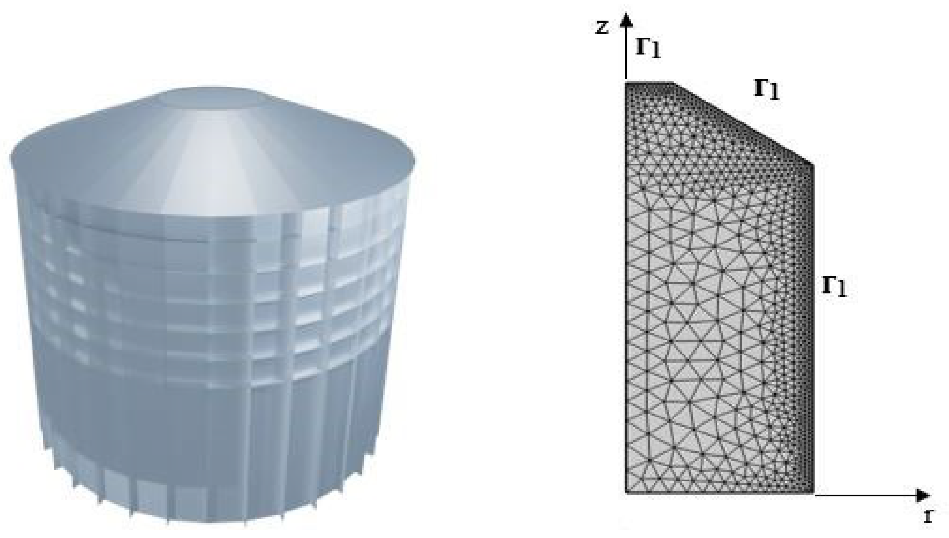
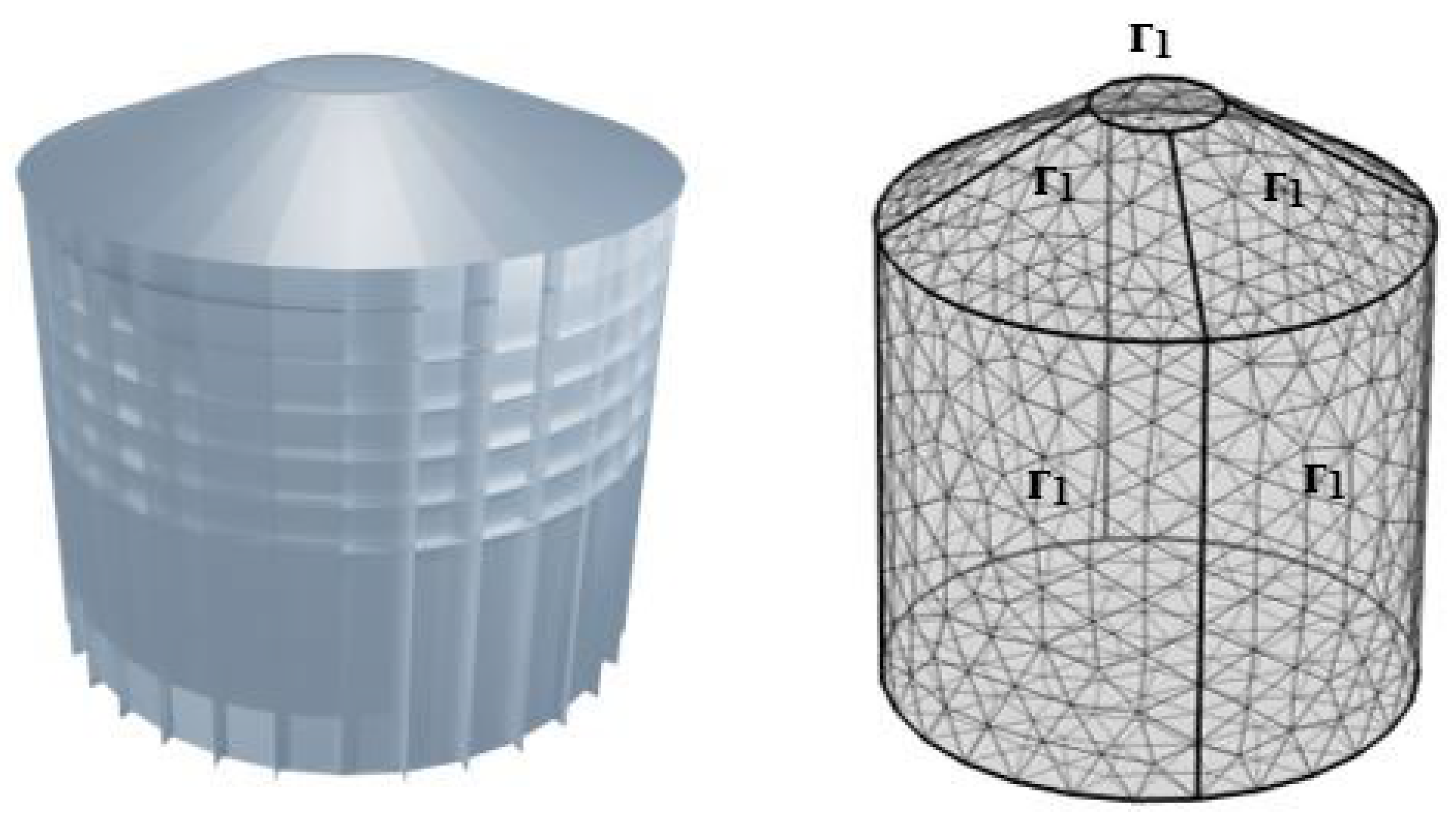
2.3. Numerical Solution

The numerical solution of the set of Equations (1)–(8), through their corresponding initial and boundary conditions, was performed using COMSOL Multiphysics^®. The domain was discretized with mesh densification along the silo walls, where the largest temperature gradients are observed, as shown in Figure 1 and Figure 2. For the 2D model resolution, finite element methods (FEMs) were used with a mesh size of 0.838 m away from the boundaries and 0.462 m at the boundaries, as shown in Figure 4. For the -D model resolution, the finite volume method (FVM) was employed, with a boundary mesh size of 0.381 m and a mesh size of 0.476 m away from the boundaries, as shown in Figure 5. The formulation of these methods can be found in Montross et al. [9,10] and Moukalled et al. [26].

The mesh independence analysis was conducted for a storage time of 24 h for both the 2D and 3D models, at coordinates (r = 0, z = 1.9) and (r = 0, θ = 1.9, z = 0), respectively, as it is impractical to perform the mesh analysis over the entire 31-day simulation period due to the high computational time required, especially for 3D models.

Table 5. Computation time for different mesh sizes in 2D and 3D.

Silo S
Model 2D		Model 3D
Mesh size	Computation time (min)	Mesh size	Computation time (min)
0.838 m 0.663 m 0.462 m 0.250 m 0.125 m	0.75 0.70 0.73 1.11 2.71	0.476 m 0.381 m 0.262 m 0.167 m ---------	37.20 18.85 29.32 43.86 ------
Silo B
Mesh size	Computation time (min)	Mesh size	Computation time (min)
0.838 m 0.663 m 0.462 m 0.250 m 0.125 m	1.03 1.01 1.50 1.20 1.68	0.476 m 0.381 m 0.262 m 0.167 m ----------	25.58 40.65 54.48 67.43 -------

compares computation times for 2D and 3D models for both silo sizes. The 2D models are solved in significantly lower computation times for both silos, making them suitable for quick simulations and cases where full three-dimensional accuracy is not strictly necessary. The 3D models, while more accurate for explaining heat and mass transfer phenomena, require considerably more computational time, especially when using finer meshes and larger silos.

All simulations were conducted using the CFD software COMSOL Multiphysics^® version 5.4, installed on a personal computer with a 13th Gen Intel(R) Core (TM) i5-13450HX 2.40 GHz processor (Intel, Santa Clara, CA, USA), 8 GB RAM, and Windows 11 Home. COMSOL Multiphysics^® uses the finite element method (FEM) to solve partial differential equations (PDEs). This method converts PDEs into algebraic equations, which are solved using the Newton–Raphson method as a nonlinear solver. For 3D problems, the finite volume method (FVM) is applied, integrating partial differential equations over each finite volume [26,27], which converts PDEs into algebraic equations that are numerically solved using the Newton–Raphson method as the default nonlinear solver.

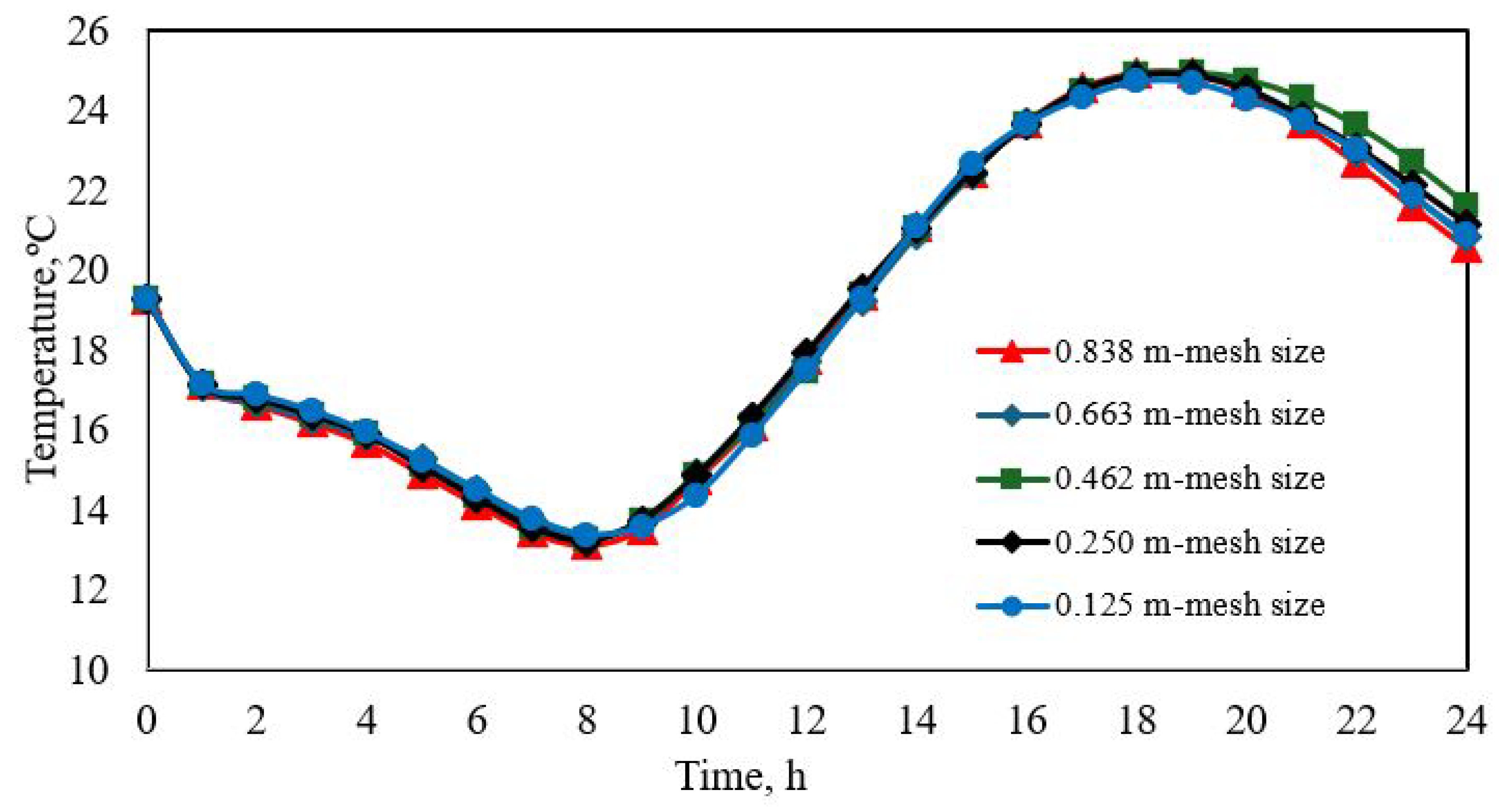
2.4. Model Validation

To confirm the model proposed in this study, the work presented by Khankari et al. [8] was used as a case study, considering a cylindrical corn storage silo with a diameter of 10 m and a height of 10 m. It is assumed that the corn is placed in this silo on 1 October with a uniform moisture content of 14% (wet basis) and a uniform temperature of 25 °C. The corn is also assumed to be stored for one year without aeration. The governing heat and mass transport equations were solved in a two-dimensional cylindrical coordinate system (r, z), assuming a symmetric domain. The energy transport equation uses time-variable boundary temperatures at the top and on the outer wall of the silo. These boundary temperatures were updated from a meteorological database at the beginning of each day. The average dry-bulb temperatures in Minneapolis/St. Paul were obtained from the monthly bulletin published by the National Climatic Data Center, based on the period from 1951 to 1980.

Additionally, to ensure the correct interpretation of the proposed mathematical model in COMSOL Multiphysics^®, we recreated the results reported by Jiménez-Islas et al. [3] with excellent agreement, both with COMSOL and with computational code in FORTRAN 90 [3].

Figure 6 shows the variation in average daily temperature for Minneapolis/St. Paul, as reported by Khankari et al. [8]. The graph shows that starting in October, temperatures decrease significantly, reaching lows near −15 °C and continuing throughout the winter months. Temperatures then gradually increase during the spring and summer, reaching levels close to 20 °C in July and August. These seasonal temperature fluctuations affect heat and moisture transfer within the silo, promoting moisture generation and the development of temperature gradients that can influence the deterioration of stored grain.

Figure 7 shows the average daily temperatures using the preloaded temperature averages in COMSOL Multiphysics^® for Guanajuato state/Bajío region (Mexico) and Minneapolis/St. Paul (USA). This graph shows that Guanajuato/Bajío exhibits a warmer and more stable climate throughout the year. Temperatures range between 15 °C and 25 °C, with less extreme variations than Minneapolis/St. Paul (USA). The thermal stability in the state of Guanajuato reduces abrupt changes in the silo’s internal conditions, decreasing moisture migration and temperature differences that could promote grain deterioration. However, higher and more persistent temperatures increase the risk of microorganisms and pest proliferation if storage is improperly managed.

Figure 8a,b compare the distribution of moisture content, stream function, and temperature isotherms reported by Khankari et al. [8] (in black and white) with those predicted by the model developed in this study (in color) for the end of the storage months of October and November. The isotherms reported by Khankari et al. [8] show that the highest temperatures in these months are in the interior of the silo. In contrast, temperatures decrease near the wall areas, following seasonal temperature fluctuations. In contrast, the isotherms predicted by the model presented in this study show quantitative and qualitative behavior like those predicted by Khankari et al. [8], with maximum temperatures at the silo center reaching 24 °C at the end of October and November. The isotherms near the silo walls also follow the same seasonal temperature fluctuations as previously reported by Khankari et al. [8].

The comparison of Figure 6, Figure 7 and Figure 8a,b exhibits that the model developed in this study allows for evaluating momentum, heat, and mass transfer during grain storage under different climatic conditions. For this reason, the developed model is shown as a versatile engineering-based tool for decision-making in grain storage worldwide.

3. Results

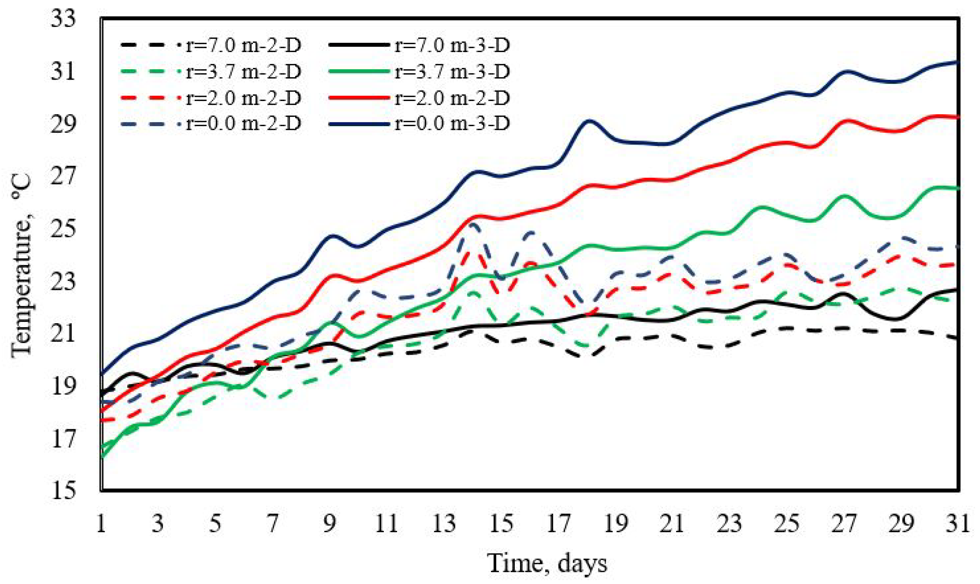
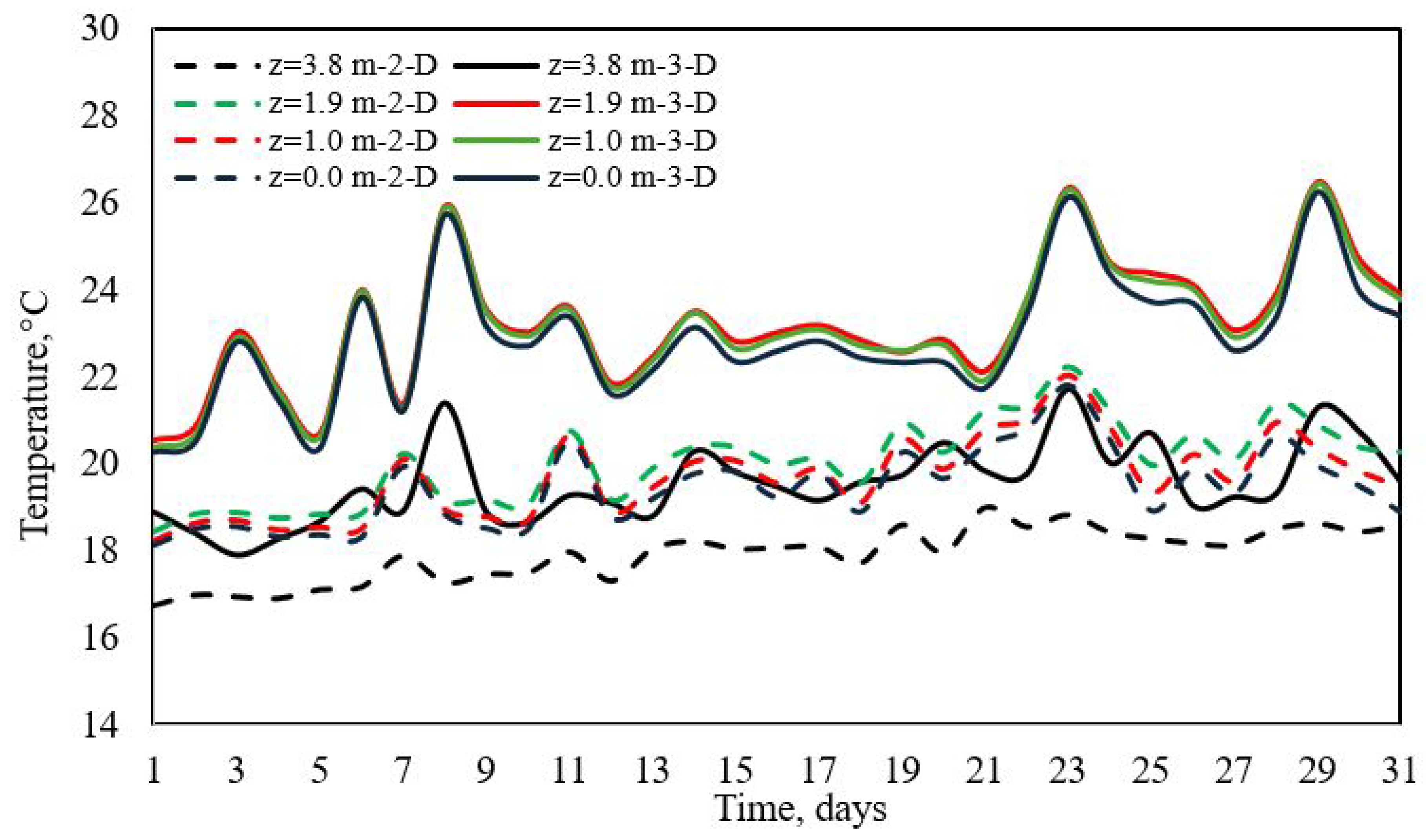
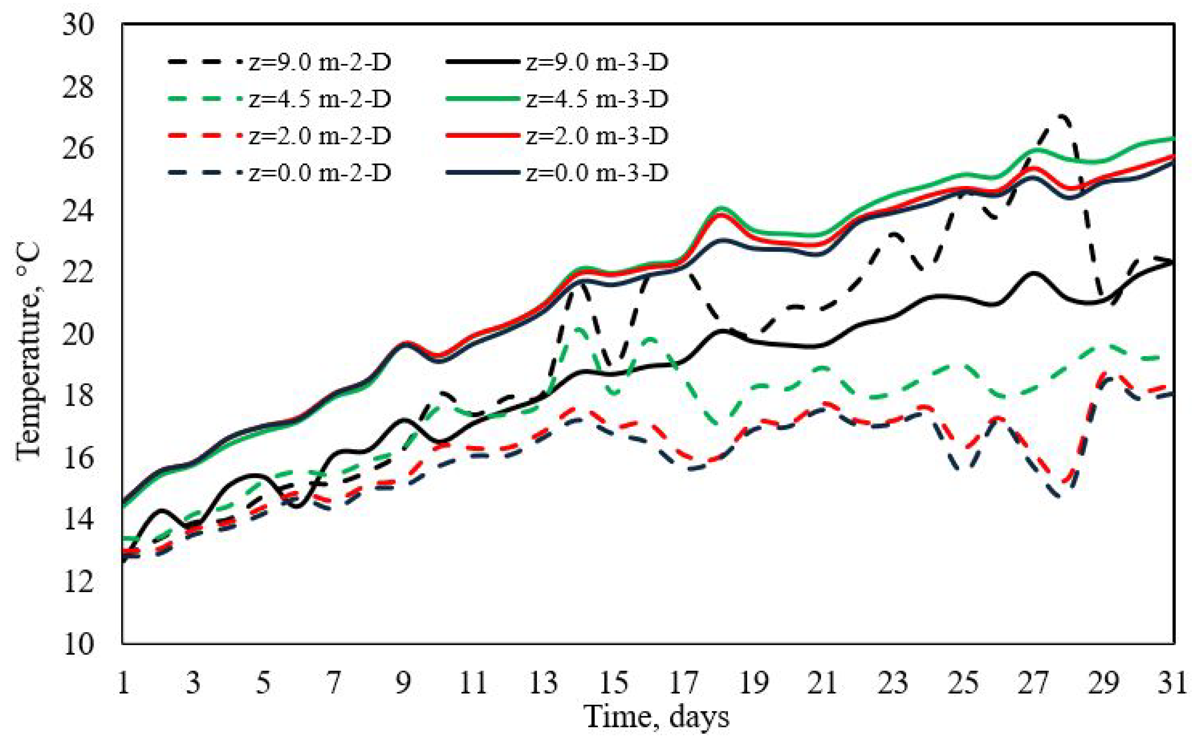
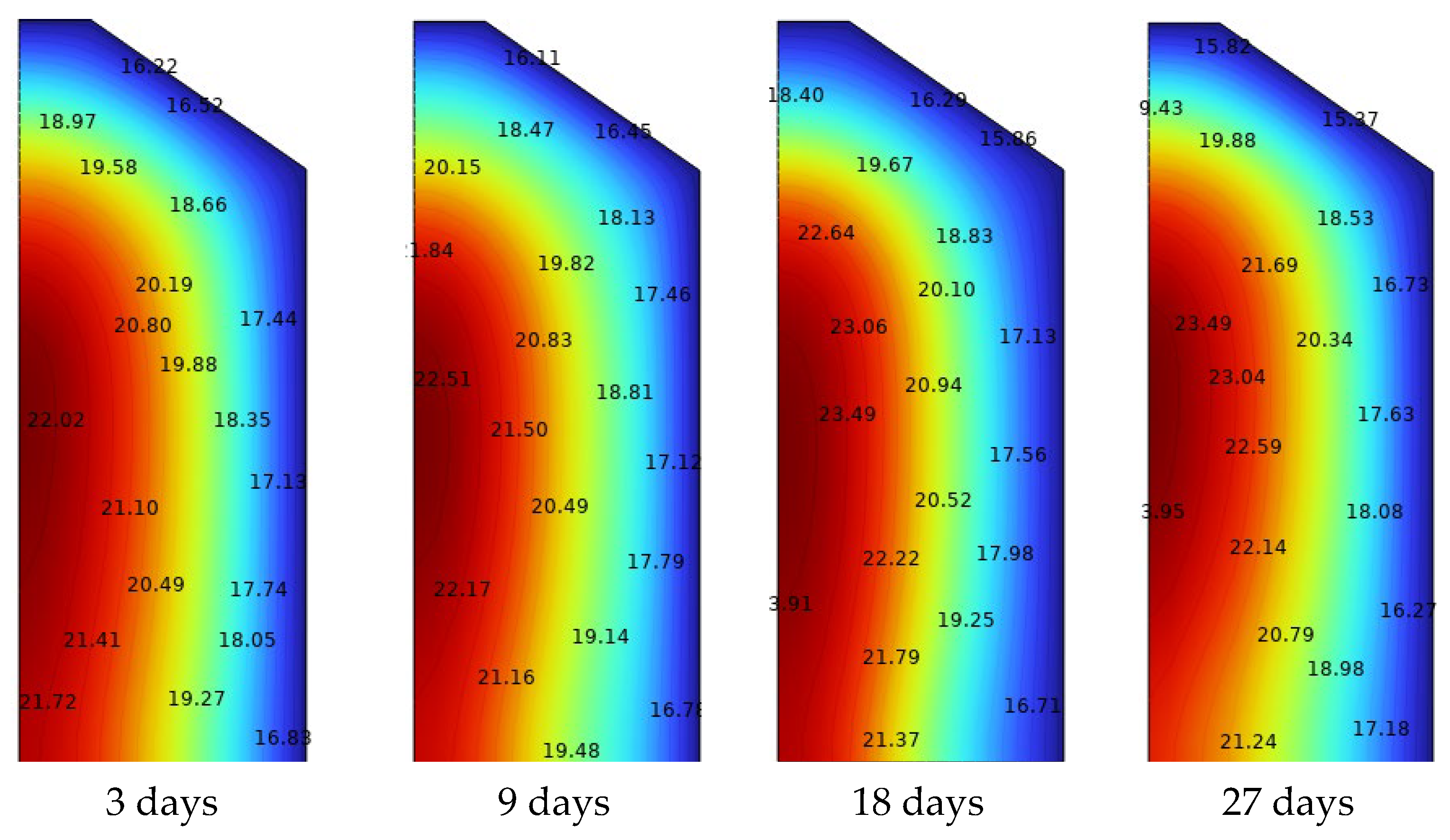
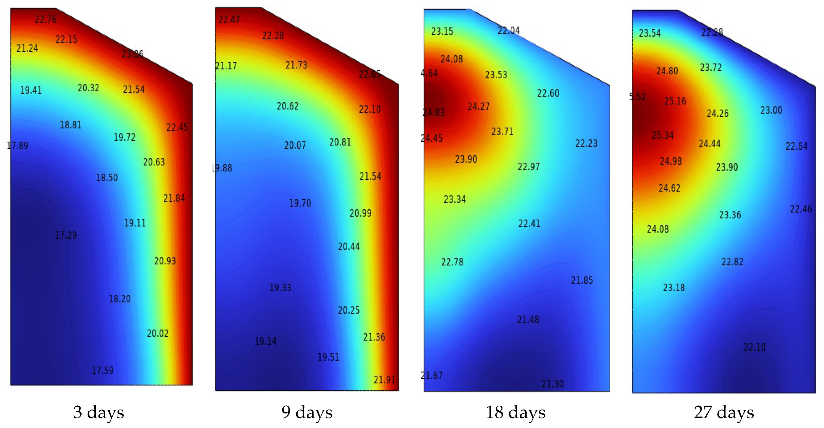
3.1. Temperature Profiles

Figure 9 shows the evolution of temperature profiles over a day of storage as predicted by the 2D and 3D models for silo S, and how ambient variation, along with solar radiation, affects temperatures inside the silo. The graph shows that the ambient temperature varies throughout the day, reaching a peak of 31 °C during the highest solar radiation hours, typically around noon or early afternoon, and then decreases in the afternoon and evening. This behavior directly affects storage temperatures, particularly in areas near the silo walls, where the highest temperatures are exhibited. This fact occurs because the grain in this zone is in direct contact with the silo walls, usually constructed of metal, which has high thermal conductivity, making it susceptible to diurnal–nocturnal temperature fluctuations and solar radiation.

During the day, the silo walls absorb heat, increasing the temperature of adjacent grain, and at night, these temperatures drop due to heat dissipation in the cooler environment. The predicted temperatures at the silo center show less variation throughout the day due to the low permeability of the grain, which acts as a natural insulator. However, heat accumulation near the silo center is due to the grain’s respiration heat and the slow heat transfer process toward the outer layers. Figure 9 also compares the predicted temperatures via 2D and 3D models. The continuous lines of the 3D model show higher temperatures and more detailed variation, particularly in the areas near the wall, while the 2D model slightly underestimates temperatures and ambient temperature fluctuations. However, the difference in the predicted maximum average temperatures between both models does not exceed one degree (0.95312 °C).

Figure 10 shows the evolution of corn grain temperature in the radial direction for silo S as predicted by the 2D and 3D models, respectively. The graph shows minimal differences between the predicted temperatures near the silo wall (r = 1.5 m), with fewer fluctuations throughout the days, consistent with diurnal–nocturnal ambient variations [4,12,15]. However, as radial positions move inward, temperatures increase for both models. The 2D model shows smoother temperature fluctuations and lower temperature peaks compared to the 3D model, suggesting that the 2D model simplifies the silo’s thermal behavior [19]. In contrast, the 3D model provides a more accurate representation of the temperature distribution inside the silo, capturing solar radiation-induced thermal variations and natural convection more effectively, with more pronounced thermal gradients and greater variability in the response across different radial positions in the silo.

Figure 11 shows the evolution of corn grain temperature in the radial direction for silo B, as predicted by the 2D and 3D models, respectively. The graph indicates a gradual increase in temperatures along the radial directions of the silo throughout the storage days, in both the 3D model (solid lines) and the 2D model (dashed lines). Throughout the storage period, temperatures show an upward trend in both models, with 3D temperatures higher than those in 2D [19]. This gradual temperature increase during storage days is related to the grain’s respiration rate; as the temperature rises, the grain’s metabolic reactions accelerate, which increases the respiration rate and, consequently, the heat generated. This phenomenon is clear in the 3D model, where heat accumulation is greater, and the volume dimension has a significant impact. While grain respiration is the primary heat source, ambient temperature variation influences storage. In a silo, solar radiation heats the walls, contributing to an overall temperature increase. The 3D model is more sensitive to these variations due to its geometry, which better captures the interaction between solar radiation and natural heat convection between the silo walls and external climatic conditions [11,15]. This explains why the 3D model’s solid lines show higher temperatures than the 2D model’s dashed lines.

For the axial temperature profiles predicted by the 3D model for silo S, Figure 12 shows a clear heat accumulation in the upper positions of the silo. This is due to natural convection, where warm air generated by grain respiration rises from the lower layers and accumulates at the top [12,16]. The 3D model captures significant variations among different axial positions within the silo. The areas closer to the silo walls (solid black line) experience less heat accumulation due to heat dissipation to the exterior.

In contrast, positions closer to the center (solid red, green, and blue lines) show a greater increase in temperature, particularly at the top, where heat accumulates and dissipates more slowly [11,23]. It is also worth noting that the lines corresponding to the bottom of the silo are flatter with smaller fluctuations, suggesting that, in this region, the temperature is more stable since warm air is rising toward the upper zones. This behavior aligns with the expected behavior of natural heat convection.

Figure 13, like Figure 12, shows the evolution of maize grain temperature in silo S for different axial positions, now at 0.93 m from the silo wall. Both figures indicate that predictions using 2D and 3D models follow the same general trends along the axial axis, regardless of the radial position. However, differences are observed in Figure 13, where temperatures are lower due to proximity to the silo walls and their exposure to ambient temperature variations [6,7,12].

Regarding the distribution of temperature profiles along the radial axis for different axial positions in silo B, Figure 14 shows trends like those in Figure 11. Both the 2D and 3D models exhibit a temperature increase comparable to that observed at the center of the silo. However, temperatures are lower near the silo walls due to their exposure to ambient temperature variations [4]. In conclusion, the temperatures along the radius of the silo are very similar in terms of trends and distribution, with slight differences in magnitudes slightly higher at the center and lower close to the wall, solely due to the influence of external environmental conditions.

Figure 15 shows the axial temperature profiles predicted for silo B. The temperature profiles calculated with the 2D model exhibit a more uniform axial profile. This reflects the simplified nature of the 2D model, which cannot adequately capture the three-dimensional variations of convection and solar radiation. The underestimation of temperature profiles by the 2D model indicates that this model is less effective in predicting heat accumulation in the upper regions of the silo [11,19,28,29]. On the other hand, the axial temperature profiles calculated with the 3D model show heat accumulation at the top of the silo. However, this accumulation is more gradual than in silo S. The temperature peaks are not as pronounced as in silo S. This effect is primarily because, in silo B, the larger total grain volume acts as a thermal buffer due to the low thermal conductivity of corn, reducing the rate at which heat rises and accumulates at the top.

The 3D model for silo B continues to capture natural convection; however, due to the greater height and mass of grain, heat dissipation towards the lower regions is slower, creating a smoother thermal gradient along the height. It is also worth noting that the axial temperature profiles predicted for the top of the silo (z = 9 m) show that temperatures predicted by the 2D model are higher than those predicted by the 3D model. This phenomenon can be explained by how three-dimensional and two-dimensional models handle heat transfer and boundary conditions. In a 3D model, heat is distributed three-dimensionally, meaning natural convection currents in the silo more realistically affect how heat moves to different regions of the silo. At the top of the silo (black line), warm air rises, but in a three-dimensional space, it also can disperse radially toward the silo walls. This phenomenon results in a more efficient dissipation effect in the 3D model, where heat moves toward the walls and dissipates into the external environment. Due to this three-dimensional distribution, the temperature at the top of the silo is lower in the 3D model than in the 2D model.

3.2. Relative Humidity Profiles

Figure 16 presents the variation in relative humidity (RH) predicted for different radial positions in silo S. The relative humidity percentages predicted by the 2D model exhibit a more uniform and less fluctuating behavior compared to the 3D model. Although the 2D model shows higher relative humidity in the center of the silo, it underestimates heat accumulation in the center, resulting in less pronounced RH at intermediate positions and near the walls compared to those predicted by the three-dimensional model. The 3D model (solid lines) shows lower RH near the silo walls [5,11,15,19,29,30]. This is because temperatures are lower near the silo walls due to heat dissipation into the environment. As a result, the grain releases less moisture in this region, leading to a lower relative humidity.

Meanwhile, at the silo center, temperatures are higher due to accumulated heat generated by grain respiration, and the RH profiles show greater fluctuations than those predicted by the 2D model. This indicates that the grain releases more moisture in this zone, increasing relative humidity.

Figure 17 shows the variations in relative humidity percentage for silo B in the radial direction. In this larger silo, the moisture content predicted by the 3D model shows a gradual and steady increase in relative humidity. Still, there are fewer fluctuations than in silo S. This signifies that in a larger silo, heat accumulates more slowly at the center, leading to a more controlled and gradual moisture release from the grain. In this silo, the temperature and humidity fluctuations for both the 2D and 3D models are not as pronounced as in silo S. Although higher temperatures at the center continue to cause increased moisture release, the magnitude of these fluctuations is lower due to the larger grain volume acting as a thermal insulator.

In general, in a larger silo, relative humidity fluctuations are less pronounced in both models, primarily due to the low thermal conductivity of the grain. However, the 3D model continues to capture the radial differences of moisture released from the grain in more detail, increasing the interstitial air humidity. In contrast, the 2D model underestimates these differences and shows a more uniform behavior [6,10,31].

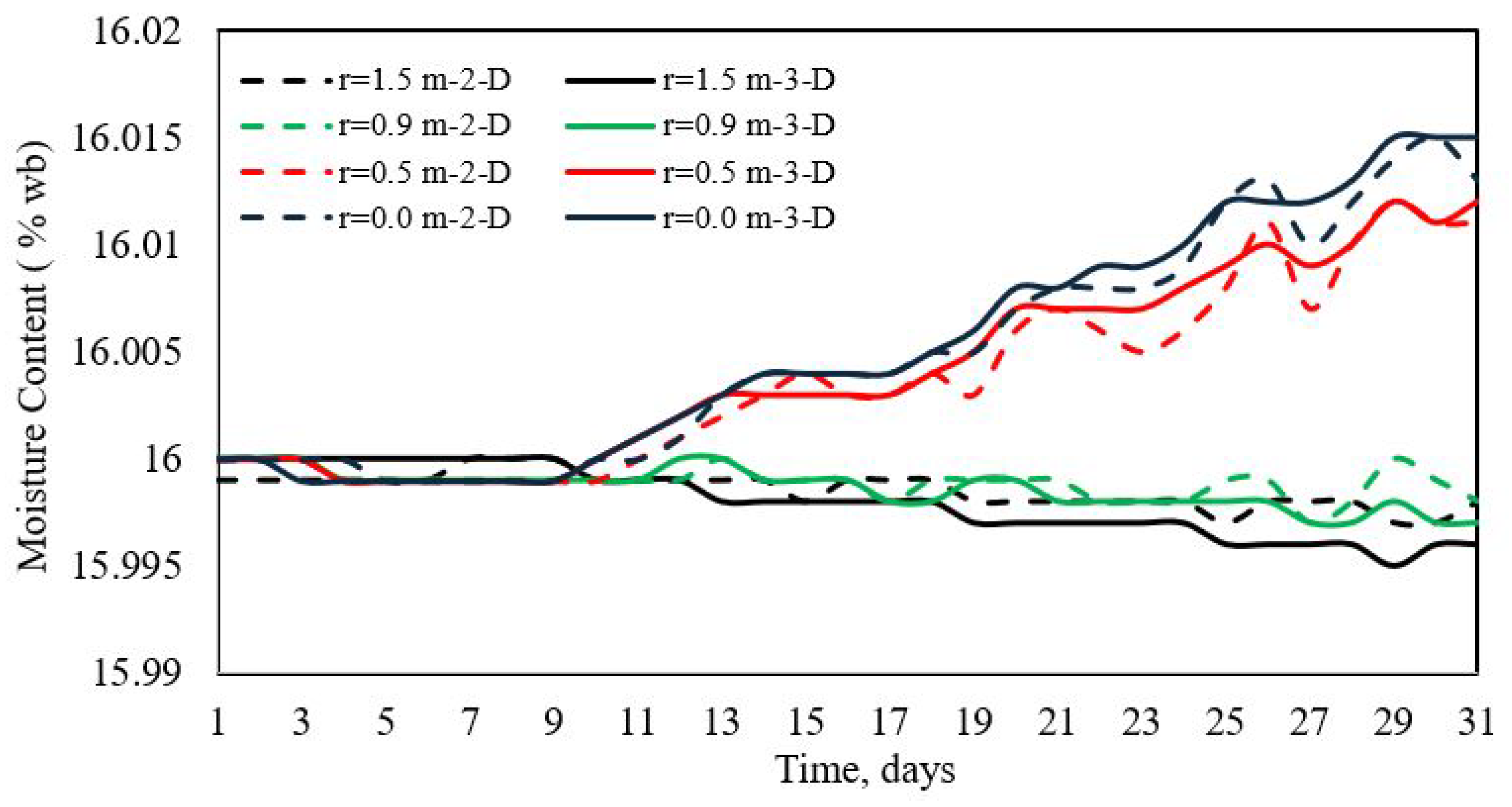
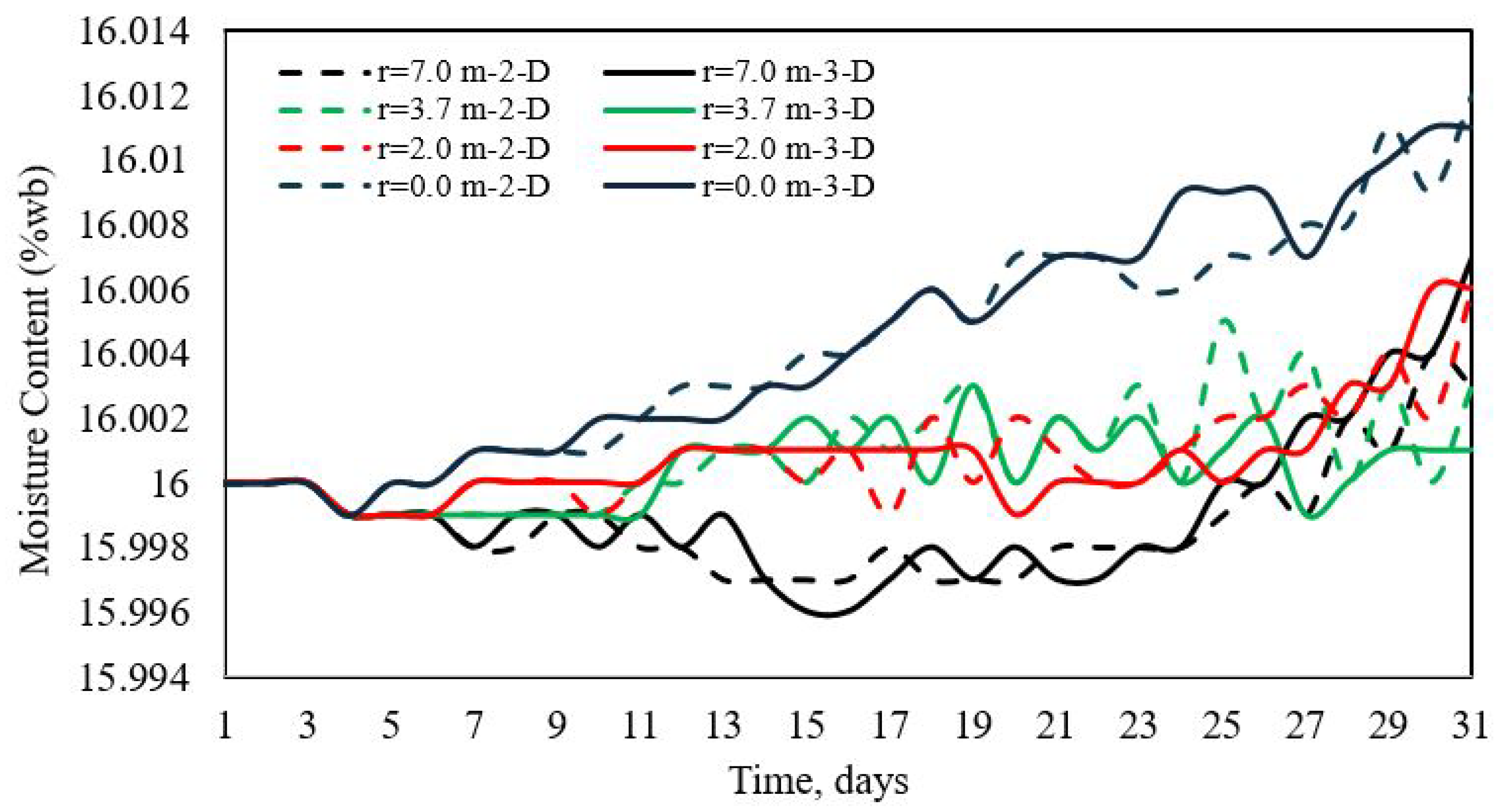
3.3. Grain Moisture Profiles

Figure 18 shows the evolution of maize grain moisture content in silo S along the radial direction. During this storage period, the values predicted by the 2D and 3D models exhibit minimal variations in grain moisture content at all radial positions. This indicates that, during the first ten days of storage, the moisture exchange between the grain and the interstitial air is minimal and relatively uniform inside the silo. However, from day 11 onward, a decreasing trend in grain moisture content is observed near the silo walls. This is the result of direct exposure to ambient temperature variations, which increases the evaporation rate of water from the grain. In contrast, the grain moisture content rises closer to the center of the silo due to the condensation of moisture generated by temperature gradients and natural convection, which concentrates water vapor in the central zone, where temperatures are more stable and less influenced by external conditions [3,6,7,12,14]. Although the 2D and 3D models show similar trends in their predictions, the 3D model is more accurate in evaluating convective and diffusive phenomena during grain storage in silos. This finding suggests that the 3D model provides a more precise description of transport phenomena and the thermal and hygrometric interactions within the silo.

Concerning the distribution of maize grain moisture content in silo B, Figure 19 presents the values predicted by the 2D and 3D models. In this case, the grain moisture content remains constant only during the first 3 days, contrasting with silo S, where moisture stability extends for a longer period. This behavior indicates that, in silo B, moisture exchanges begin more quickly due to the larger grain volume. Unlike silo S, where the moisture content progressively decreases near the walls, silo B exhibits a pattern of increase and decrease during the first 19 days, followed by a continuous rise. These fluctuations result from wider temperature gradients in silo B, generating more pronounced cycles of evaporation and condensation near the walls. Like silo S, the moisture content in the central zone increases, although more gradually and continuously in this case. Moisture accumulation in the center is due to condensation caused by vapor migration from the walls and intermediate zones toward the center, where temperatures are more stable. In the intermediate zones, the moisture content shows a more fluctuating behavior compared to silo S, oscillating between the conditions near the walls and the central zone [3,6,7,12,14]. This behavior highlights the complex interaction between natural convection, mass transfer, and temperature distribution in these regions. While both models predict similar qualitative and quantitative behavior, the 3D model offers higher resolution and accuracy, particularly for larger silos or under conditions with significant thermal and moisture gradients.

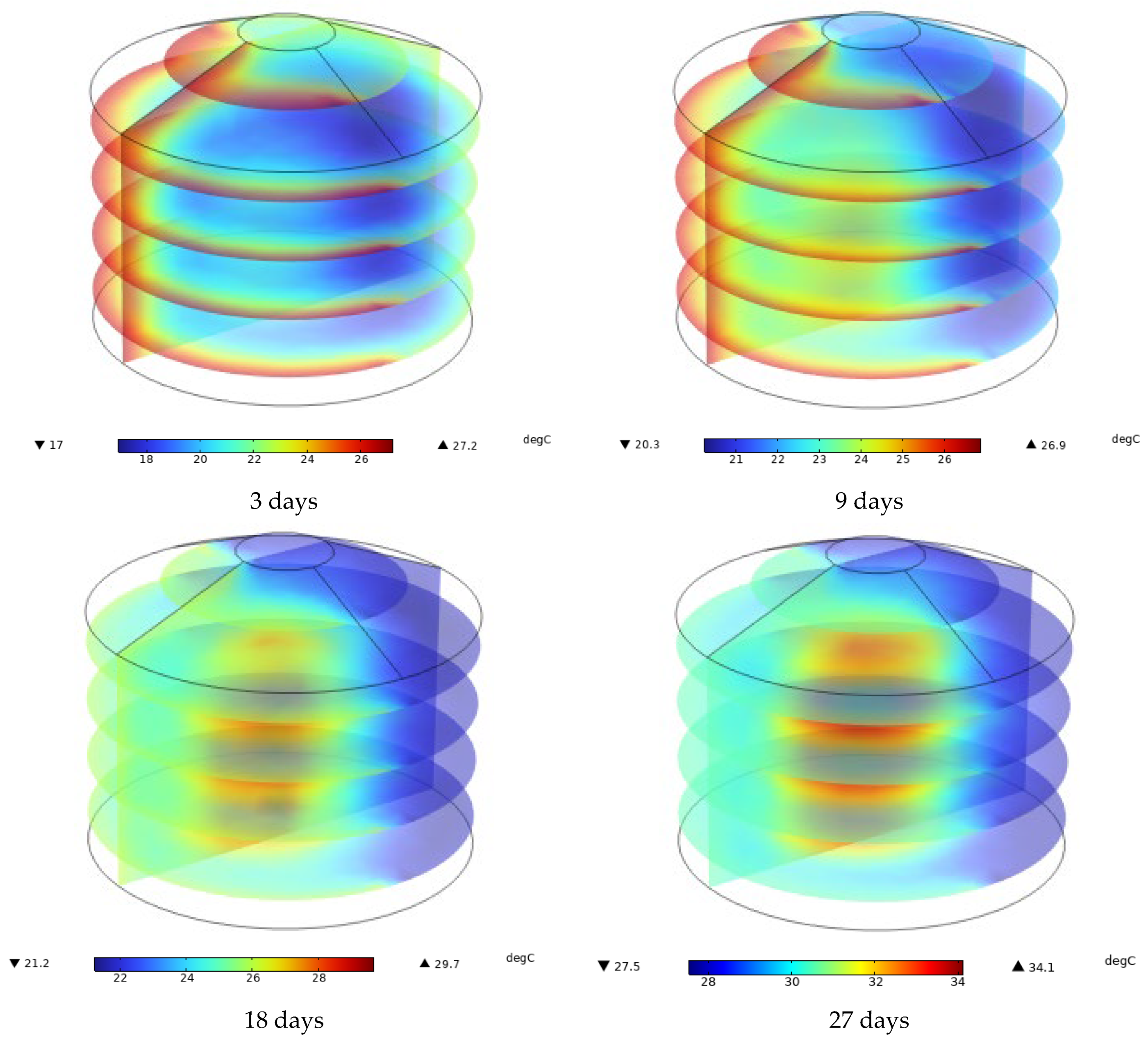
3.4. Temperature Contours

Figure 20 exhibits the temperature contours predicted by a 2D model for silo S. It is important to note that the blue color in the following figures represents the lowest temperatures. In contrast, the red color represents the highest temperatures. At the beginning of the process, during the first 3 days of storage, the center of silo 1 shows the formation of a hot core. This reflects heat accumulation. Meanwhile, areas near the walls (blue and green areas) are cooler due to heat dissipation toward the exterior of the silo. By day 9 of storage, the hot core has expanded, indicating that heat is accumulating and spreading more widely within the silo, and green areas (representing intermediate temperatures) occupy more space.

On day 18 of storage, the natural convection phenomenon is fully developed, with warm air continuously rising from the center of the silo to the upper region. In contrast, cooler air near the walls descends [8,10,12,13]. This phenomenon reaches its maximum extent by the end of July, reducing temperature differences between the center and intermediate positions. Over time, the system tends toward thermal equilibrium. However, temperature differences between the center and the walls persist, keeping natural convection and air streams active.

Figure 21 shows the temperature contours predicted by the 3D model for silo S, where heat accumulation in the silo center is also observed. However, the three-dimensional model displays both the axial and radial distribution of heat, with greater heat accumulation in the upper areas of the silo compared to the lower part. Additionally, the areas near the walls show more complex gradients, reflecting how natural heat convection and solar radiation impact temperatures near the walls in a three-dimensional manner. By day 9 of storage, natural convection already distributes heat from the center to the upper areas, which is more apparent in the 3D view.

On day 18 of storage, the heat started to distribute more uniformly along the entire height of the silo. Still, the upper region remains most affected by solar radiation, and the intermediate areas showed greater heat accumulation than those near the ground [5,11,19]. On day 27 of storage, the upper region of the silo still exhibits higher temperatures than the lower ones, reflecting the sustained effect of solar radiation. The center of the silo remains the hottest region, but the three-dimensional heat distribution is more distinct [5,11,22].

Figure 22 shows the temperature contours for silo B as predicted by the 2D model. The temperature contours during the first few days of storage indicate that the silo walls are the areas most affected by solar radiation, creating a nearby red contour at the top and along the walls, while the center of the silo remains cooler [8,12,16,31]. By day 9 of storage, heat has begun to spread toward the center of the silo, although the walls and upper areas remain warmer. The radial gradient remains evident, with regions near the walls warmer than the center. By day 18 of storage, heat has further distributed from the center toward the upper part of the silo. Still, the model does not capture the temperature variation along the silo’s height. At the end of the storage period, a state is reached where heat accumulates in the upper region of the silo, with a temperature difference of approximately 3.0 °C.

Finally, Figure 23 shows the temperature contours predicted by the 3D model for silo B. At the start of the process, heat accumulation is concentrated in the upper areas and near the walls, where solar radiation has an immediate effect, and it can be observed how the heat generated at the walls begins to move radially toward the center. By day 9 of storage, heat accumulation is evident in the upper areas, providing a more detailed view of how heat is distributed radially and axially. Convection and solar radiation in 3D show how the highest temperatures are concentrated in the upper region of the silo; this effect is not evident in the 2D model [19].

By day 18 of storage, heat has been distributed in layers along the silo’s axial axis, with the upper areas still hotter due to the continuous effect of solar radiation. Natural convection has also redistributed part of the heat toward the upper and central regions [5,6,11,12,30]. At the end of July, convective currents have balanced the temperature within the silo, with zones near the walls dissipating some of the heat generated by grain respiration to the exterior, creating a thermal gradient between the center and the walls. The upper areas remain the hottest due to constant solar exposure and heat accumulation in the rising air [5,11].

3.5. Stream Function Contours

Figure 24 describes the 2D and 3D stream flow patterns for silo S at the end of the storage period. These flow patterns correspond to natural convection, where the closed lines represent the air paths. For the 2D model, the flow pattern exhibits a primary counterclockwise cycle. The higher intensity of the streamlines near the axial axis indicates a steeper velocity gradient in this region, where the air moves faster due to heating and the resulting reduction in density. In contrast, lower streamline values near the outer wall correspond to the return flow region, where air descends more slowly, influenced by the ambient temperature. In the case of the 3D model, more intricate flow patterns are observed, distributed throughout the silo volume. The metabolic heat generated by the grain emerges as the primary circumstance of convective flow, intensifying the upward movement of hot air and altering the overall flow distribution. While the flow distribution in the 2D model is predominantly influenced by wall-imposed boundary conditions, the 3D model demonstrates that metabolic heat plays a more significant role, resulting in a flow that more accurately represents the movement of interstitial air. This highlights the greater representativeness of the three-dimensional analysis for capturing natural convection within the silo.

Figure 25 illustrates the 2D and 3D stream flow patterns for silo B at the end of the storage period. The 2D model depicts a dominant convective flow cycle with counterclockwise motion. Warm air generated near the walls, driven by ambient temperature variations, exhibits greater intensity, resulting in an upward flow consistent with the characteristics of a larger silo, where an increased height and radius amplify the ambient temperature effects. In contrast, the 3D model reveals a more dynamic flow structure, with warm air predominantly rising in the silo center, primarily driven by the metabolic heat generated by the grain. The air descends near the walls due to ambient cooling, forming multiple recirculation cells distributed throughout the silo’s volume. This demonstrates a more complex interaction of airflow pathways compared to the simpler patterns predicted by the 2D model. The two-dimensional analysis simplifies the storage process by focusing on the axial flow behavior, which neglects radial dynamics. This limitation restricts the representation of air movement and the interactions between different regions within the silo. Conversely, the three-dimensional analysis captures these interactions, providing a more accurate depiction of flow behavior. It highlights the critical role of the silo core as a zone for the accumulation of heat and moisture, offering valuable insights for understanding and optimizing storage conditions.

4. Discussion

In this study, 2D and 3D mathematical models were developed to predict the temperature and humidity distribution within a stored mass of maize grains in a cylindrical silo with a conical roof. The results revealed that grains near the silo walls follow the diurnal–nocturnal and seasonal fluctuations in ambient temperature [6,32]. Moreover, when considering heat production from grain metabolism as a function of temperature and humidity, the maximum storage temperatures reached 34 °C by the end of May. This finding aligns closely with the report by Andrade et al. [32], which documented a maximum temperature of 35 °C during maize storage in a cylindrical silo after 160 days of storage. This three-dimensional model accounted for the effects of ambient temperature variations and solar radiation and was applied to simulate the temperature distribution within a maize-filled silo in Brazil. These results confirm the hypothesis of this study, which states that solar radiation and ambient temperature variations significantly influence the temperature and humidity distribution within silos. Additionally, the proposed model has practical implications, as it can be adapted to diverse types of grains and climatic conditions, making it globally relevant to the grain storage and trading industry.

Lastly, an important direction for future research is to incorporate and evaluate the effect of aeration in the three-dimensional models developed for storage silos. This would allow for the analysis of how controlled airflow can influence the temperature and humidity distribution within the silo, particularly under variable climatic conditions. Furthermore, it would be relevant to study the optimization of aeration periods, airflow rates, and the distribution of entry points to enhance grain preservation and reduce the risk of pest and fungal proliferation. This approach could complement the current analysis, which only considers the influences of solar radiation and ambient temperature variations.

5. Conclusions

This study developed and compared two-dimensional (2D) and three-dimensional (3D) mathematical models to predict temperature and moisture dynamics in unventilated corn storage silos. Both models incorporated critical factors such as external temperature fluctuations, solar radiation, and grain respiration, enabling a comprehensive analysis of heat and mass transfer phenomena during storage.

The 3D model demonstrated superior accuracy in capturing thermal gradients and moisture distribution throughout the silo, particularly in regions away from the walls and areas near the walls influenced by solar radiation and environmental variations. For smaller silos (silo S), the percentage difference in average temperature predictions between the two models was less than 14%, whereas, for larger silos (silo B), the difference did not exceed 17%, highlighting that both models effectively analyze grain storage conditions despite their differing levels of detail. However, the 3D model provides greater precision in representing complex heat and mass transfer phenomena, making it essential for studies involving large silos where thermal inertia and geometric effects are significant.

Despite the increased computational cost and resource demands of the 3D model, the 2D model proved computationally efficient, with simulation times averaging 1.2 min compared to 43.86 min for the 3D model. This makes the 2D model a practical tool for rapid preliminary assessments, while the 3D model remains indispensable for detailed evaluations requiring high accuracy. Both models exhibited similar general trends in temperature and humidity variation over time, demonstrating their utility for silo design and optimization. Future research should focus on incorporating dynamic boundary conditions, such as wind effects, and analyzing the aeration effects to optimize grain storage conditions further. Additionally, experimental validation with multi-depth temperature and moisture measurements would enhance the models’ accuracy and applicability under diverse climatic conditions. This dual modeling approach highlights the complementary strengths of the 2D and 3D models, providing robust tools for improving grain storage strategies worldwide.

References

1. Babangida, L.Y.; Yong, H. Design development and techniques for controlling grains post-harvest losses with metal silo for small and medium scale farmers. AJB 2011, 10, 14552–14561. [Google Scholar] [CrossRef]
2. Sutton, A.O.; Strickland, D.; Norris, D.R. Food storage in a changing world: Implications of climate change for food-caching species. Clim. Change Responses 2016, 3, 12. [Google Scholar] [CrossRef]
3. Jiménez-Islas, H.; Navarrete-Bolaños, J.L.; Botello-Álvarez, E. Numerical study of the natural convection of heat and 2-D mass of grain stored in cylindrical silos. Agrociencia 2004, 38, 325–342. [Google Scholar]
4. Barreto, A.; Abalone, R.; Gastón, A. Mathematical modelling of momentum, heat and mass transfer in silos: Part I: Model development and validation. Lat. Am. Appl. Res. 2013, 43, 377–384. [Google Scholar]
5. Lawrence, N.J.; Maier, N.D.E.; Stroshine, N.R.L. Three-dimensional transient heat, mass, momentum, and species transfer in the stored grain ecosystem: Part I. Model Development and Evaluation. Trans. ASABE 2013, 56, 179–188. [Google Scholar] [CrossRef]
6. Barreto, A.A.; Abalone, R.; Gastón, A. Mathematical modelling of momentum, heat and mass transfer in grains stored in silos: Part II: Model application. Lat. Am. Appl. Res. 2013, 43, 385–391. [Google Scholar]
7. Khankari, N.K.K.; Morey, N.R.V.; Patankar, N.S.V. Mathematical model for moisture diffusion in stored grain due to temperature gradients. Trans. ASABE 1994, 37, 1591–1604. [Google Scholar] [CrossRef]
8. Khankari, N.K.K.; Morey, N.R.V.; Patankar, N.S.V. Application of a numerical model for prediction of moisture migration in stored grain. Trans. ASABE 1995, 38, 1789–1804. [Google Scholar] [CrossRef]
9. Montross, M.D.; Maier, N.D.E.; Haghighi, K. Validation of a finite element stored grain ecosystem model. Trans. ASABE 2002, 45, 1465. [Google Scholar] [CrossRef]
10. Montross, M.D.; Maier, D.E.; Haghighi, N.K. Development of a finite-element stored grain ecosystem model. Trans. ASABE 2002, 45, 1455. [Google Scholar] [CrossRef]
11. Lawrence, N.J.; Maier, D.E.; Stroshine, N.R.L. Three-dimensional transient heat, mass, momentum, and species transfer in the stored grain ecosystem: Part II. Model Validation. Trans. ASABE 2013, 56, 189–201. [Google Scholar] [CrossRef]
12. Quemada-Villagómez, L.I.; Molina-Herrera, F.I.; Carrera-Rodríguez, M.; Calderón-Ramírez, M.; Martínez-González, G.M.; Navarrete-Bolaños, J.; Jiménez-Islas, H. Numerical study to predict temperature and moisture profiles in unventilated grain silos at prolonged periods. Int. J. Thermophys. 2020, 41, 52. [Google Scholar] [CrossRef]
13. Abbouda, N.S.K.; Chung, N.D.S.; Seib, N.P.A.; Song, N.A. Heat and mass transfer in stored milo. Part I. Heat Transfer Model. Trans. ASABE 1992, 35, 1569–1573. [Google Scholar] [CrossRef]
14. Abbouda, N.S.K.; Seib, N.P.A.; Chung, N.D.S.; Song, N.A. Heat and mass transfer in stored milo. Part II. Mass Transfer Model. Trans. ASABE 1992, 35, 1575–1580. [Google Scholar] [CrossRef]
15. Abalone, R.; Gastón, A.; Cassinera, R.; Lara, M. Modelización de la distribución de la temperatura y humedad en granos almacenados en silos. Mecánica Comput. 2006, 24, 233–247. [Google Scholar]
16. Carrera-Rodríguez, M.; Martínez-González, G.M.; Navarrete-Bolaños, J.L.; Botello-Álvarez, J.E.; Rico-Martínez, R.; Jiménez-Islas, H. Transient numerical study of the effect of ambient temperature on 2-D cereal grain storage in cylindrical silos. J. Stored Prod. Res. 2011, 47, 106–122. [Google Scholar] [CrossRef]
17. Jiang, N.S.; Jofriet, N.J.C. Finite element prediction of silage temperatures in tower silos. Trans. ASABE 1987, 30, 1744–1750. [Google Scholar] [CrossRef]
18. Jofriet, J.C.; Jiang, S.; Tang, S. Finite element prediction of temperature gradients in walls of cylindrical concrete storage structures. Can. J. Civ. Eng. 1991, 18, 12–19. [Google Scholar] [CrossRef]
19. Alagusundaram, N.K.; Jayas, N.D.S.; White, N.N.D.G.; Muir, N.W.E. Three-dimensional, finite element, heat transfer temperature distribution model in grain storage bins. Trans. ASABE 1990, 33, 0577–0584. [Google Scholar] [CrossRef]
20. Rocha, K.S.O.; Martins, J.H.; Martins, M.A.; Saraz, J.A.O.; Filho, A.F.L. Three-Dimensional modeling and simulation of heat and mass transfer processes in porous media: An application for maize stored in a flat bin. Dry. Technol. 2013, 31, 1099–1106. [Google Scholar] [CrossRef]
21. Bartosik, N.R.E.; Maier, N.D. Effect of airflow distribution on the performance of NA/LT in-bin drying of corn. Trans. ASABE 2006, 49, 1095–1104. [Google Scholar] [CrossRef]
22. Novoa-Muñoz, F. Simulation of the temperature of barley during its storage in cylindrical silos. MATCOM 2019, 157, 1–14. [Google Scholar] [CrossRef]
23. Markowski, M.; Bialobrzewski, I.; Bowszys, J.; Suchecki, S. Simulation of temperature distribution in stored wheat without aeration. Dry. Technol. 2007, 25, 1527–1536. [Google Scholar] [CrossRef]
24. De Oliveira, G.H.; De Oliveira, A.P.L.R.; Correa, P.C. Use of the CFD tool to analyze the aeration compartment in a horizontal silo. Int. J. Agric. Technol. 2022, 2, 1–6. [Google Scholar] [CrossRef]
25. Valle, F.J.M.; Gastón, A.; Abalone, R.M.; De la Torre, D.A.; Castellari, C.C.; Bartosik, R.E. Study and modelling the respiration of corn seeds (Zea mays L.) during hermetic storage. Biosyst. Eng. 2021, 208, 45–57. [Google Scholar] [CrossRef]
26. Masud, A.; Khurram, R.A. Multiscale finite element method for the incompressible Navier–Stokes equations. Comput. Methods Appl. Mech. Eng. 2006, 195, 1750–1777. [Google Scholar] [CrossRef]
27. Moukalled, F.; Mangani, L.; Darwish, M. The Finite Volume Method in Computational Fluid Dynamics: An Advanced Introduction with OpenFOAM® and MATLAB; Springer International Publishing: Cham, Switzerland, 2016. [Google Scholar] [CrossRef]
28. Jia, C.; Sun, D.; Cao, C. Finite element prediction of transient temperature distribution in a grain storage bin. J. Agric. Eng. Res. 2000, 76, 323–330. [Google Scholar] [CrossRef]
29. Jia, C.; Sun, D.; Cao, C. Computer simulation of temperature changes in a wheat storage bin. J. Stored Prod. Res. 2001, 37, 165–177. [Google Scholar] [CrossRef]
30. Gastón, A.; Abalone, R.; Cassinera, A.; Lara, M.A. Predicción de la distribución de temperatura de granos almacenados en silos. AVERMA 2005, 9, 13–18. [Google Scholar]
31. Abe, T.; Basunia, M. Simulation of temperature and moisture changes during storage of rough rice in cylindrical bins owing to weather variability. J. Agric. Eng. Res. 1996, 65, 223–233. [Google Scholar] [CrossRef]
32. Andrade, N.E.T.; Couto, N.S.M.; Queiroz, N.D.M.; Faroni, N.L.R.A.; De Sousa Damasceno, N.G. Three-Dimensional Simulation of the Temperature Variation in Corn Stored in Metallic Bin. In Proceedings of the 2002 ASAE Annual Meeting, Chicago, IL, USA, 28–31 July 2002. [Google Scholar] [CrossRef]
Figure 1. Geometric system and computational domain for the 2D model.
Modelling 06 00007 g001
Figure 2. Geometric system and computational domain for the 3D model.
Modelling 06 00007 g002
Figure 3. Variation in average ambient temperature and average solar radiation for the state of Guanajuato throughout the months of the year.
Modelling 06 00007 g003
Figure 4. Effect of mesh size on the temperature profile prediction at the center of silo S in 2D.
Modelling 06 00007 g004
Figure 5. Effect of mesh size on the temperature profile prediction at the center of silo S in 3D.
Modelling 06 00007 g005
Figure 6. Average daily temperature variations for Minneapolis/St. Paul, as reported by Khankari et al. [8].
Modelling 06 00007 g006
Figure 7. Comparison of average daily temperatures reported by Khankari et al., 1995 [8], for the state of Minneapolis/St. Paul versus average daily temperatures for Guanajuato state/Bajío region.
Modelling 06 00007 g007
Figure 8. (a) Comparison of moisture content, stream function, and temperature by Khankari et al. [8] versus those predicted by the model presented in this study at the end of October; (b) Comparison of moisture content, stream function, and temperature by Khankari et al. [8] versus those predicted by the model presented in this study at the end of November.
Modelling 06 00007 g008aModelling 06 00007 g008b
Figure 9. Temperature profiles at different radial positions during a day of storage at the center of silo S.
Modelling 06 00007 g009
Figure 10. Temperature profiles at different radial positions over a month of storage at the center of silo S.
Modelling 06 00007 g010
Figure 11. Temperature profiles at different radial positions over a month of storage at the center of silo B.
Modelling 06 00007 g011
Figure 12. Temperature profiles at different axial positions over a month of storage at the center of silo S.
Modelling 06 00007 g012
Figure 13. Temperature profiles at different axial positions over a month of storage at r = 0.93 m from the silo S wall.
Modelling 06 00007 g013
Figure 14. Temperature profiles at different axial positions over a month of storage at r = 3.25 m from the silo B wall.
Modelling 06 00007 g014
Figure 15. Temperature profiles at different axial positions over a month of storage at the center of silo B.
Modelling 06 00007 g015
Figure 16. Relative humidity profiles at different radial positions over a month of storage at the center of silo S.
Modelling 06 00007 g016
Figure 17. Relative humidity profiles at different radial positions over a month of storage at the center of silo B.
Modelling 06 00007 g017
Figure 18. Distribution of maize grain moisture content at different radial positions over a month of storage at over a month of storage at the center of silo S.
Modelling 06 00007 g018
Figure 19. Distribution of maize grain moisture content at different radial positions over a month of storage at over a month of storage at the center of silo B.
Modelling 06 00007 g019
Figure 20. Temperature contours during corn storage in silo S in 2D.
Modelling 06 00007 g020
Figure 21. Temperature contours during corn storage in silo S in 3D.
Modelling 06 00007 g021aModelling 06 00007 g021b
Figure 22. Temperature contours during corn storage in silo B in 2D.
Modelling 06 00007 g022
Figure 23. Temperature contours during corn storage in silo B in 3D.
Modelling 06 00007 g023
Figure 24. Distribution of the stream function (m3/day) during corn storage in silo S in 2D and 3D.
Modelling 06 00007 g024
Figure 25. Distribution of the stream function (m3/day) during corn storage in silo B in 2D and 3D.
Modelling 06 00007 g025