
Hydrodynamic Modeling of Unstretched Length Variations in Nonlinear Catenary Mooring Systems for Floating PV Installations in Small Indonesian Islands


 , , , , and
Abstract
:1. Introduction

2. Materials and Methods
2.1. Model Description and Material Properties
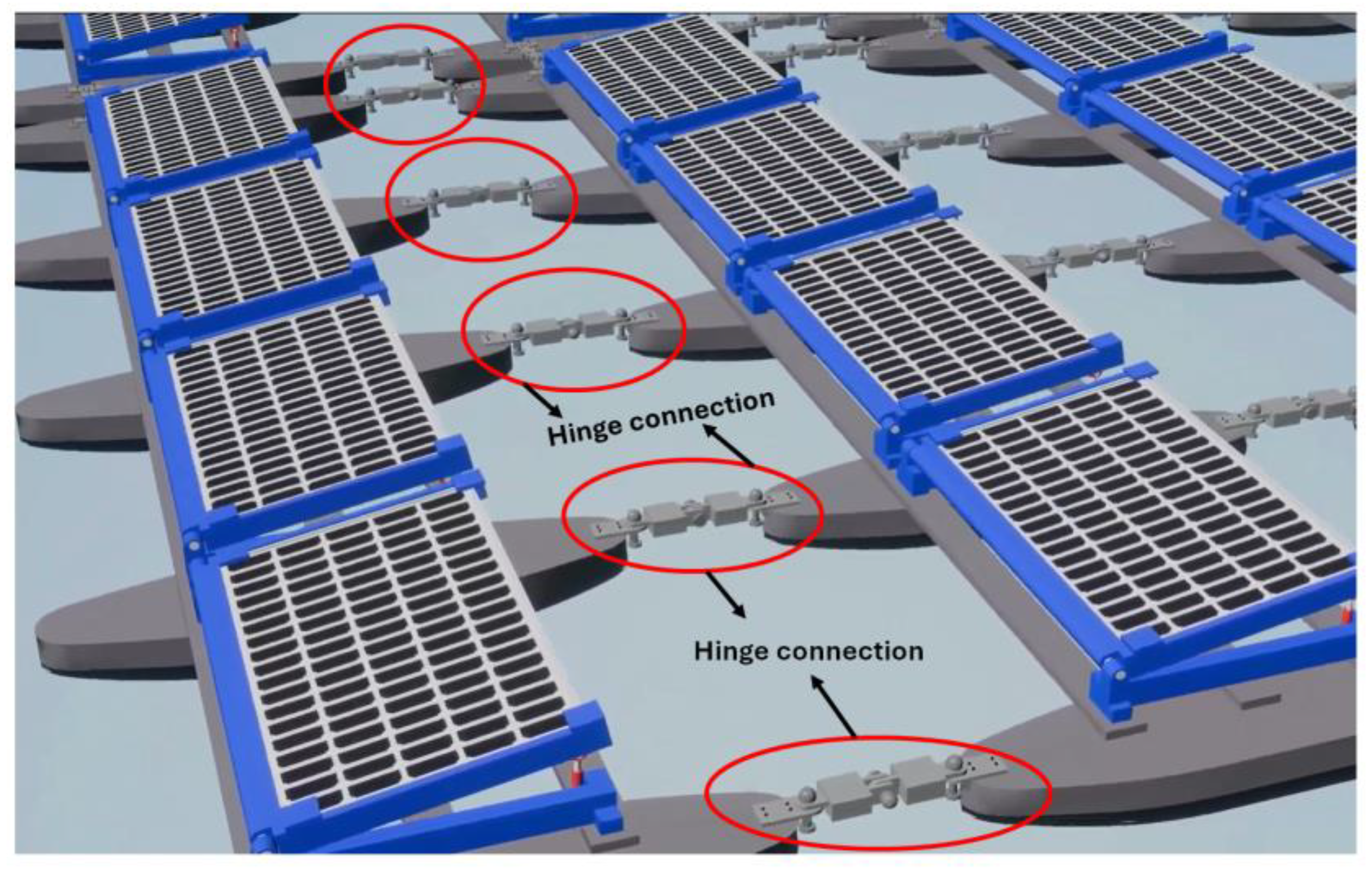
2.2. Mooring Properties and Arrangements
2.3. Boundary Element Method Governing Equations
2.4. Dynamic Catenary Cable Equations
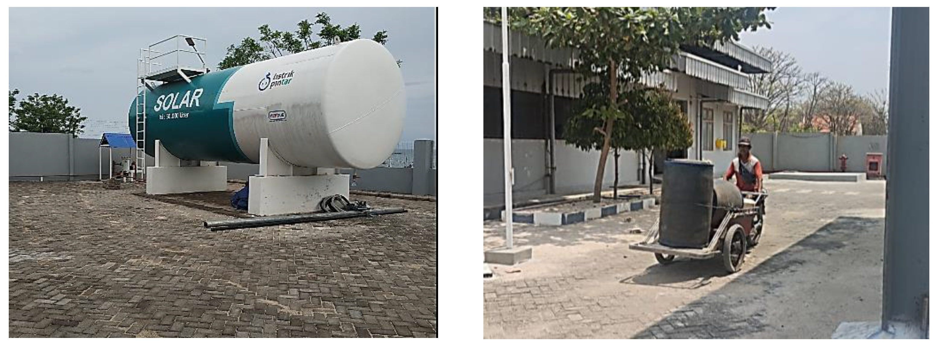
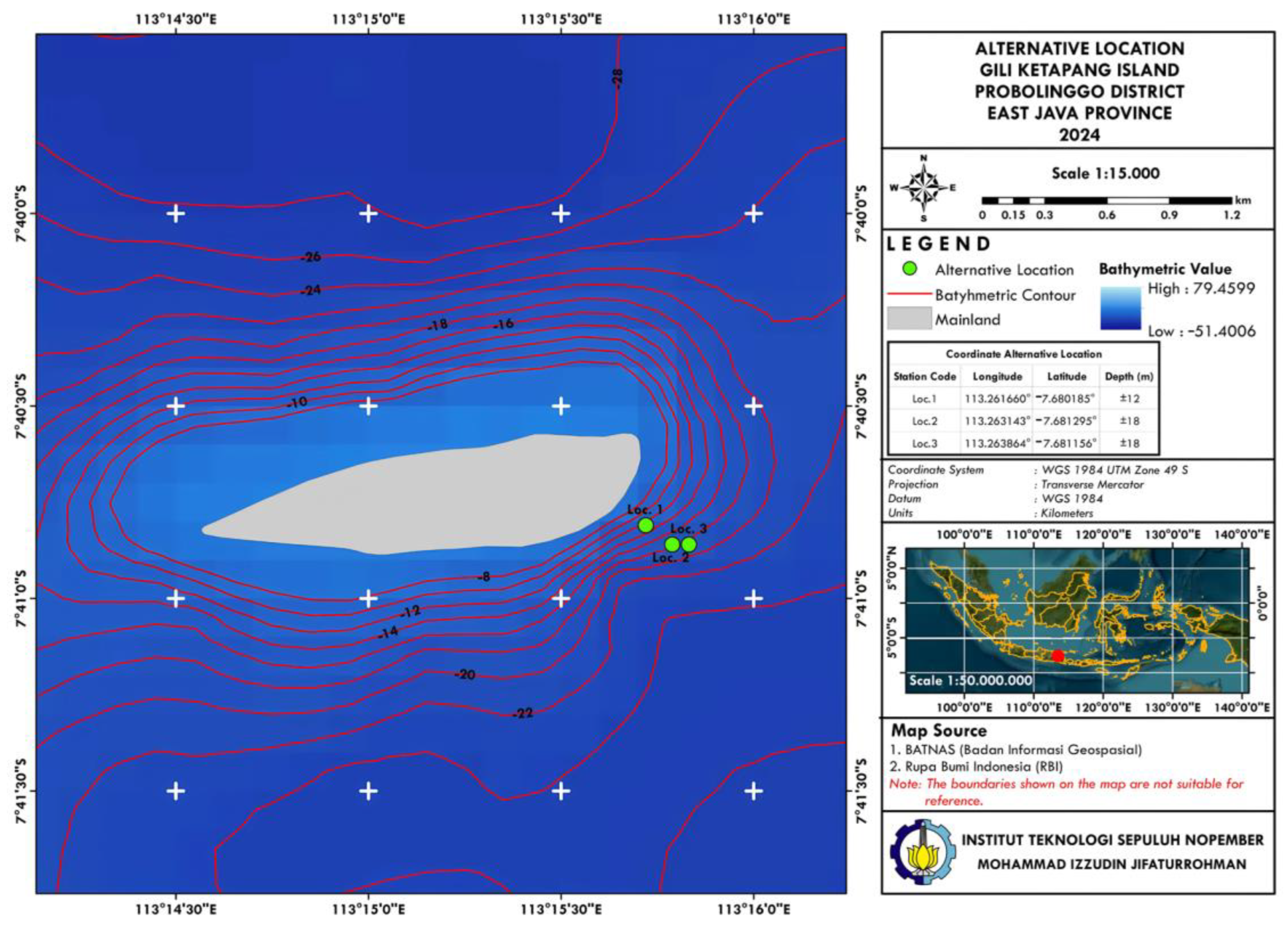
2.5. Case Study: Gili Ketapang Island
2.6. Bathymetry and Environmental Data in Gili Ketapang’s Water
2.7. Grid Convergence Index
- (1)
- : Grid divergence
- (2)
- : Oscillatory convergence
- (3)
- : Monotonic convergence
3. Result and Discussion
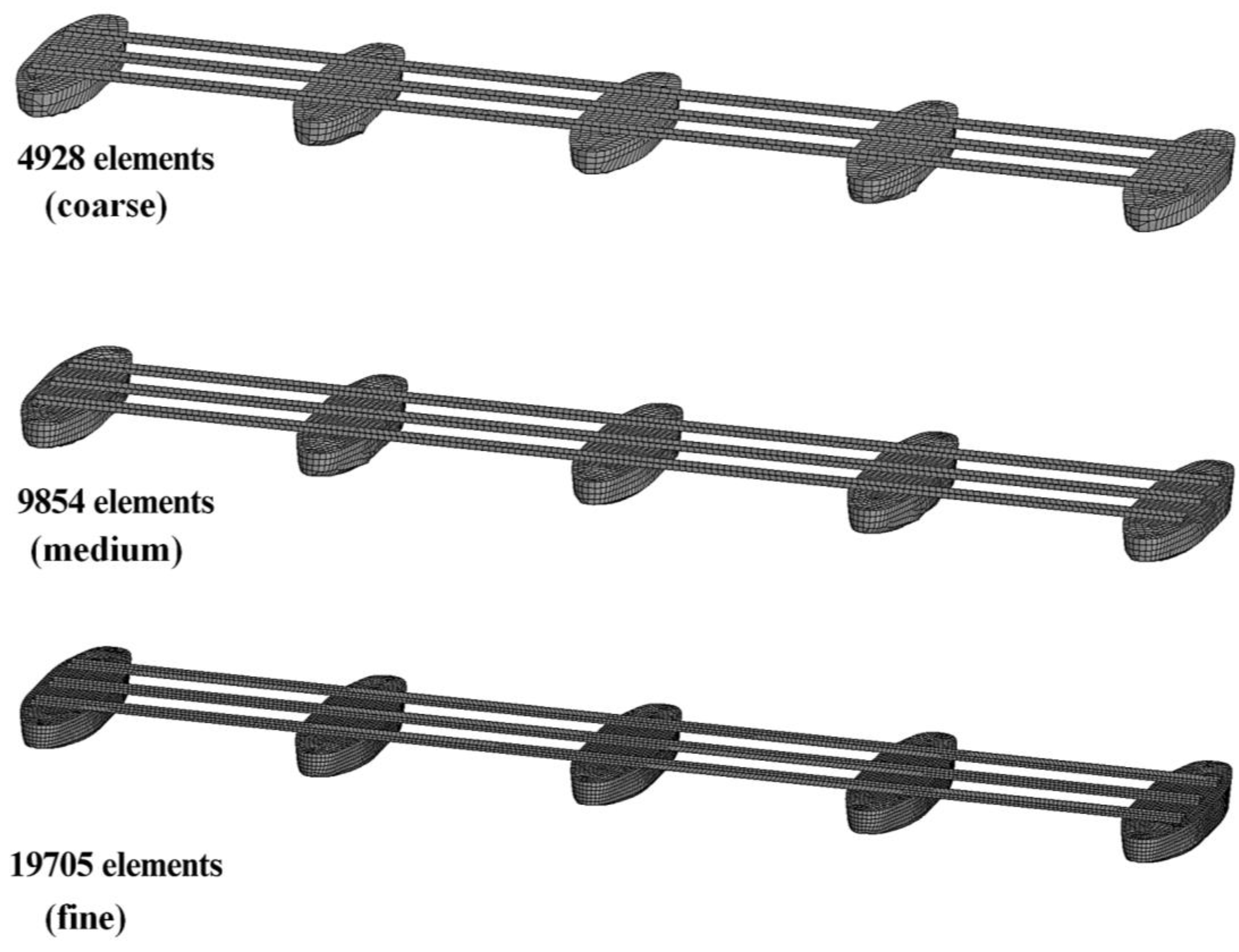
3.1. Mesh Discretization and Numerical Stability
3.2. Structural Motions in Frequency Domain
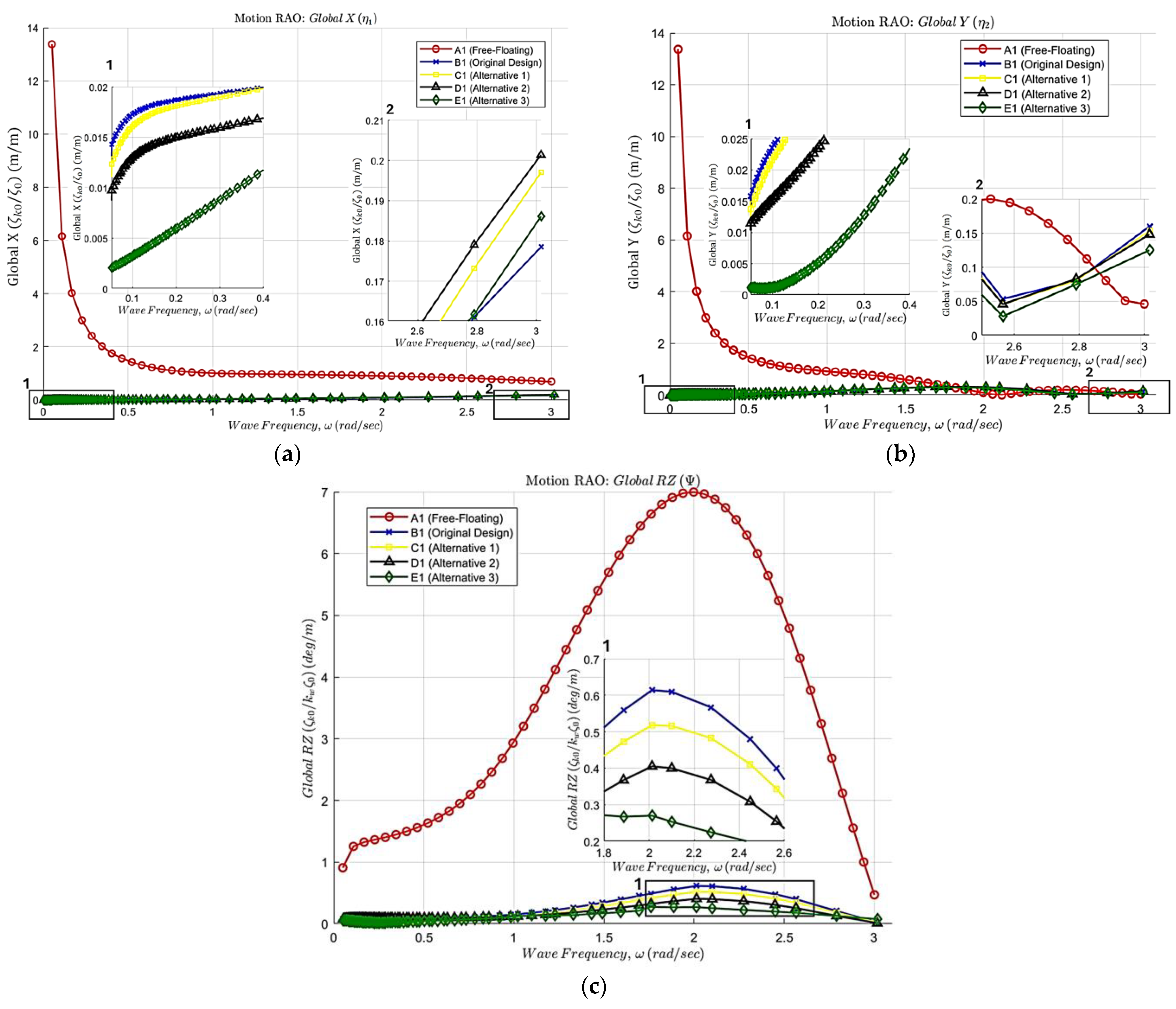
3.2.1. Horizontal Motions in Regular Waves
3.2.2. Pure Oscillatory Motions in Regular Waves
3.3. Structural Horizontal Motions Response in Time Domain
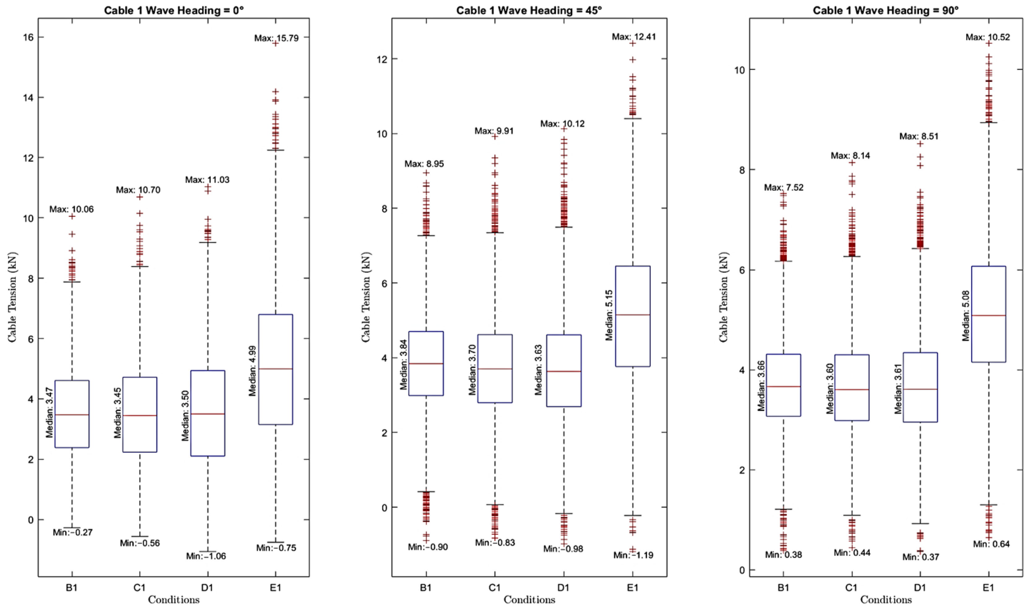
3.4. Time Domain in Mooring Line Tension
4. Conclusions
- Achieving numerical stability involved conducting a GCI calculation between the medium and fine grid sizes. The results showed that both variables, heave and pitch RAO, had differences of less than 1%, indicating no significant differences between the medium and fine mesh sizes. Therefore, this study employed the medium grid size (19,705 elements) to reduce computation time.
- External restoring forces and moments generated by the mooring system significantly reduce horizontal motion displacements (surge, sway, and yaw). The reduction exceeds 90%, with the MAPE in RAO calculations showing reductions of 94.01% in surge, 99.78% in sway, and 96.19% in yaw between free-floating and moored conditions. Furthermore, a shortened in unstretched mooring length leads to a decrease in motion excitation in RAO, though the effect is not highly significant. Even with a length reduction of up to 51% of the original design, the motion response remains relatively stable. This is evidenced by the RMSE values, which indicate minimal differences in motion between the longest and shortest mooring configurations: 0.01 m/m for surge, 0.02 m/m for sway, and 0.09 deg/m for yaw.
- For pure oscillatory motion, which is governed by natural hydrostatic restoring forces and moments, the addition of a mooring system has a combined effect in restricting motion. The MAPE values for heave, roll, and pitch RAOs are 7.96%, 6.29%, and 28.16%, respectively. This indicates that although the mooring system contributes to motion reduction, its effect is less significant compared to the reduction observed in horizontal displacements.
- The time-domain response for horizontal motion shows a declining trend in motion, indicating improved performance in mooring stiffness as the mooring length decreases. Additionally, of the three motion responses, the most significant reduction occurs in rotational motion (yaw), rather than in translational motions (surge and sway).
- In the time domain, mooring lines with the same properties and configurations show stronger nonlinearity in restoring forces and stiffness as the mooring length decreases. This increased nonlinearity causes a wider distribution of line tension data, resulting in larger maximum mooring tensions. Nevertheless, all mooring cables across all wave headings still meet the safety requirements, as all actual tension values remain below the allowable limit of 30.69 kN.
5. Future Work
Author Contributions
Funding
Data Availability Statement
Conflicts of Interest
Nomenclature
| ABS | American Bureau Shipping | FoS | Factor of Safety |
| AWP | Water Plane Area | FPV | Floating Photovoltaics |
| B | Breadth | GCI | Grid Convergence Index |
| B1 | Demihull Width | GHI | Global Horizontal Irradiation |
| BEM | Boundary Element Method | GML | Longitudinal Metacentric Height |
| Cb | Block Coefficient | GMT | Transverse Metacentric Height |
| CoG | Center of Gravity | H | Height |
| Cp | Prismatic Coefficient | Ha | Hectare |
| Cs | Ocean Current Velocity | HAT | Highest Astronomical Tide |
| DNV | Det Norske Veritas | HDPE | High-Density Polyethylene |
| E | Modulus Young | HHWL | Highest High Water Level |
| EA | Axial Stiffness | Hs | Significant Wave Height |
| F | Formzahl number | i, j, k | Unit vector with respect to x-, y- and z-axis, respectively |
| FEM | Finite Element Method | IBIEM | Indirect Boundary Integral Equation Method |
| IEA | International Energy Agency | RMSE | Root Mean Square Errors |
| IQR | Inter-Quartile Range | RX, θ | Roll motion mode |
| IWRC | Independent Wire Rope Core | RY, φ | Pitch motion mode |
| JONSWAP | Joint North Sea Wave Project | RZ, Ψ | Yaw motion mode |
| KB | Keel to Buoyancy | S | Spacing |
| km | Kilo meter | T | Draft |
| kN | Kilo Newton | Tamax | Allowable Tension Maximum |
| kW | Kilo Watt | Tp | Peak Wave Period |
| Kxx | X-Axis of radius gyration | UTM-WGS | Universal Transverse Mercator—World Geodetic System |
| Kyy | Y-Axis of radius gyration | V | Velocity vector |
| Kzz | Z-Axis of radius gyration | Wd−1 | Original water depth |
| LAT | Lowest Astronomical Tide | Wd−2 | Conservative water depth |
| LCB | Longitudinal Center of Buoyancy | Weff | Effective Weight |
| LCOE | Levelized Cost of Electricity | Wv | Wind speed |
| LLWL | Lowest Low Water Level | Ws*h | Catenary Weight |
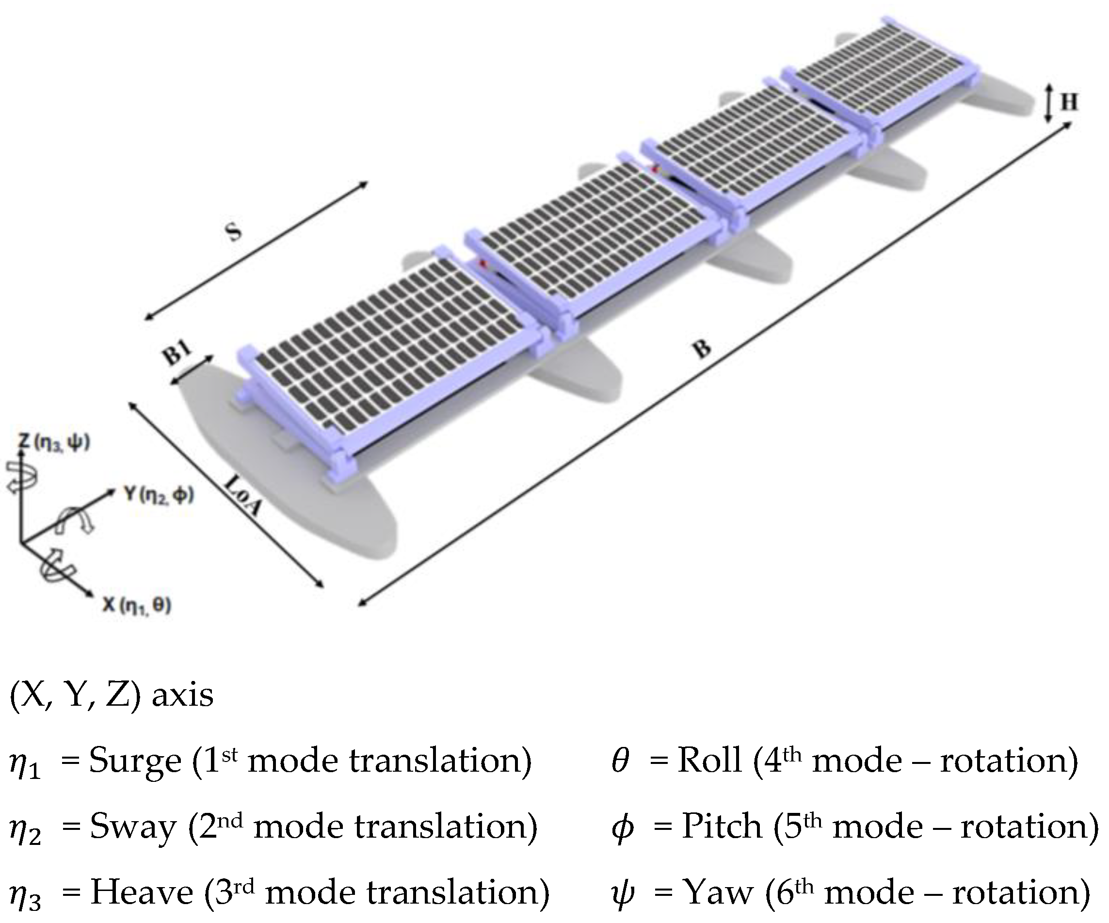
| LMM | Lump-Mass Method | X, η1 | Surge motion mode |
| LoA | Length over All | Y, η2 | Sway motion mode |
| m | Meter | Z, η3 | Heave motion mode |
| m/s | Meter per second | Z0 | Mean sea level |
| MAPE | Mean Absolute Percentage Error | Radiation damping coefficient | |
| MBL | Minimum Breaking Load | Hydrostatic stiffness coefficient | |
| mm | millimeter | External hydrodynamic loading vector per unit length | |
| MW | Mega Watt | Diffraction forces (forces from waves scattered by the structure) | |
| Ni | Number of cells used in numerical setup | Incident wave forces (forces due to incoming waves) | |
| PM | Pierson–Moskowitz | damping coefficient of the j-th segment of the cable line | |
| Q1 | First quartile, or the 25th percentile | approximate relative error between medium and fine grids | |
| Q2 | Second quartile, or the 50th percentile | Bending Stiffness | |
| Q3 | Third quartile, or the 75th percentile | derived order of the method | |
| RAOs | Response Amplitude Operators | Distributed moment per unit length | |
| JONSWAP spectrum | refinement factors | ||
| ω | Wave frequency | Element’s weight per unit length | |
| Peak wave frequency | The difference area under heave and pitch RAO Curves between the medium and fine grids | ||
| Laplace equation | The difference area under heave and pitch RAO Curves between the coarse and medium grids | ||
| Element length at node j | Axial strain in node j | ||
| original length of the j-th segment | Amplitude of vessel motion in the j-th mode | ||
| Ø | Diameter | Spatial derivative of shear force vector | |
| γ | Peak enhancement factor | Partial derivatives of potential velocity function with respect to u, v, and w | |
| Δ | Displacement | extrapolated value between medium and fine grids | |
| Inertial force of per unit length | Gradient operator | ||
| spectral width parameter | Tension force | ||
| Potential velocity function | Gravitational acceleration | ||
| Spatial derivative of bending moment vector | Vessel mass matrix (physical mass of the structure) | ||
| Moment due to shear force | Added mass matrix (additional inertia due to surrounding fluid) | ||
| Spatial derivative of tension force vector along the cable element | grid refinement ratio |
References
- Esparza, I.; Olábarri Candela, Á.; Huang, L.; Yang, Y.; Budiono, C.; Riyadi, S.; Hetharia, W.; Hantoro, R.; Setyawan, D.; Utama, I.K.A.P.; et al. Floating PV Systems as an Alternative Power Source: Case Study on Three Representative Islands of Indonesia. Sustainability 2024, 16, 3145. [Google Scholar] [CrossRef]
- Majumder, A.; Kumar, A.; Innamorati, R.; Mastino, C.C.; Cappellini, G.; Baccoli, R.; Gatto, G. Cooling Methods for Standard and Floating PV Panels. Energies 2023, 16, 2439. [Google Scholar] [CrossRef]
- Cai, S.; Bao, G.; Ma, X.; Wu, W.; Bian, G.B.; Rodrigues, J.J.; Albuquerque, V.H.C. Parameters Optimization of the Dust Absorbing Structure for Photovoltaic Panel Cleaning Robot Based on Orthogonal Experiment Method. J. Clean. Prod. 2019, 217, 724–731. [Google Scholar] [CrossRef]
- Cazzaniga, R.; Rosa-Clot, M. The Booming of Floating PV. Sol. Energy 2021, 219, 3–10. [Google Scholar] [CrossRef]
- International Energy Agency. World Energy Outlook 2024. Available online: https://www.iea.org/data-and-statistics/charts/world-electricity-generation-in-the-stated-policies-scenario-2010-2035 (accessed on 10 January 2024).
- Wang, Z.; Carriveau, R.; Ting, D.S.K.; Xiong, W.; Wang, Z. A Review of Marine Renewable Energy Storage. Energy Rep. 2019, 5, 4444. [Google Scholar] [CrossRef]
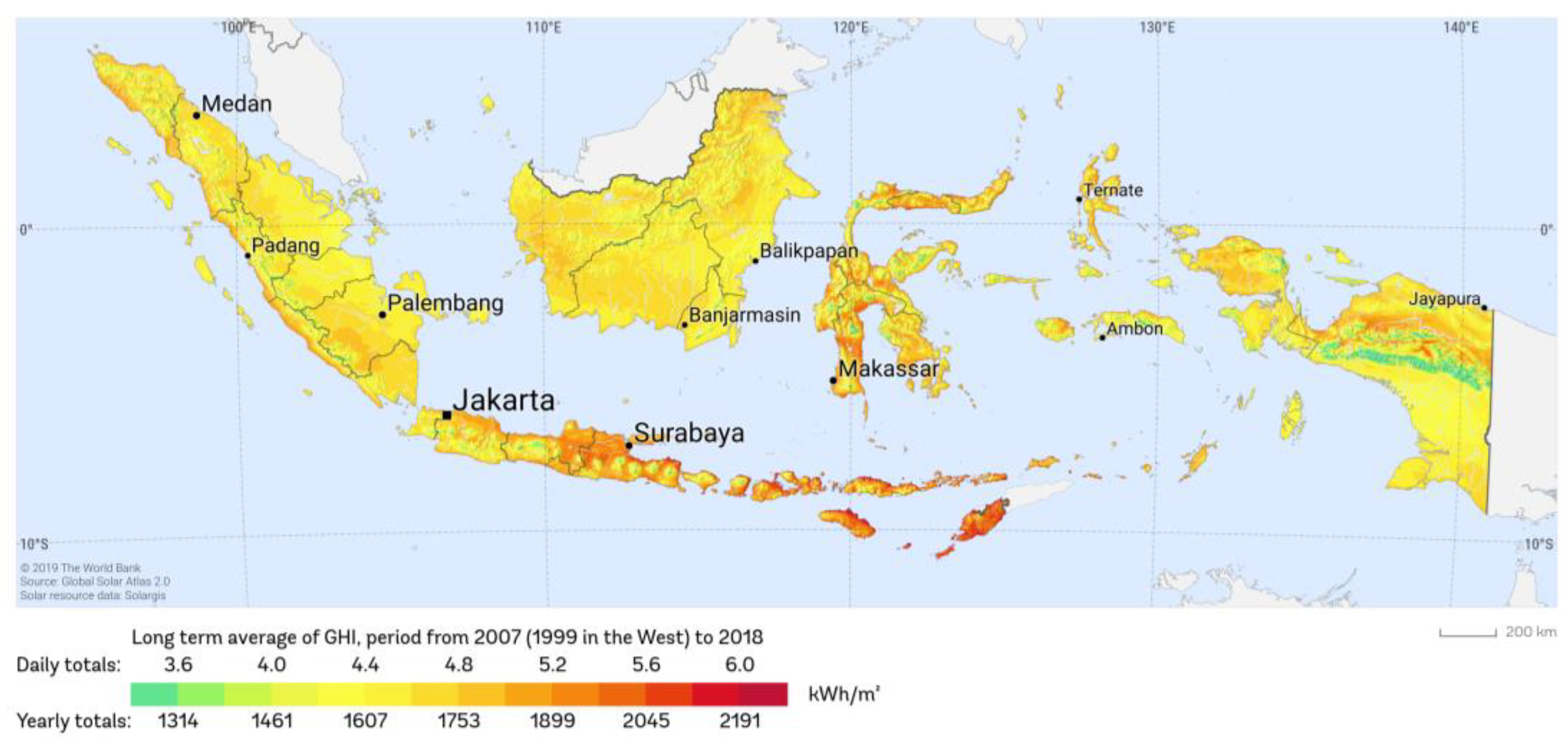
- Solargis. Global Horizontal Irradiation in Indonesia. SolarGIS. Available online: https://solargis.com/maps-and-gis-data/download/indonesia (accessed on 27 June 2024).
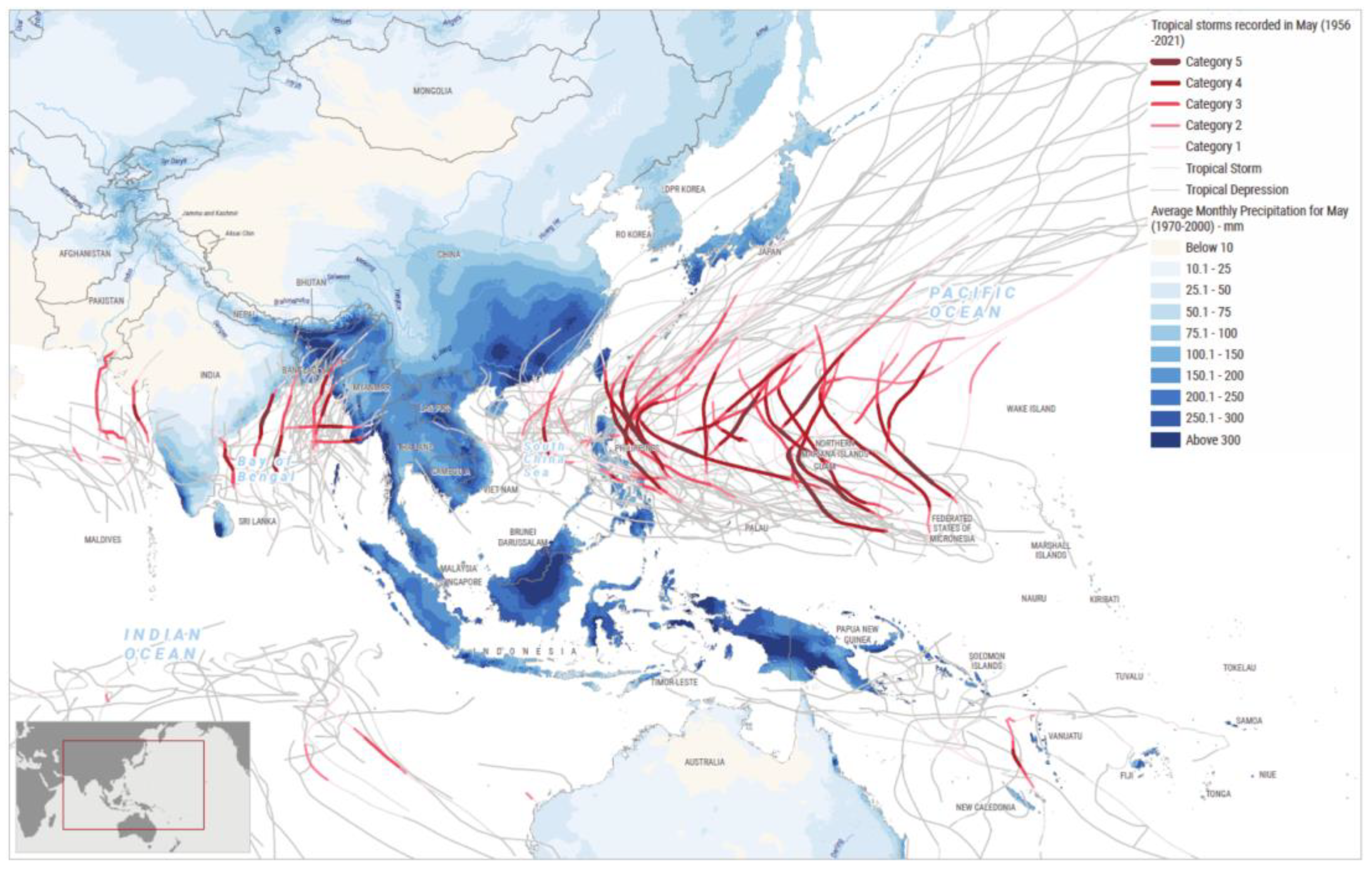
- Office for the Coordination of Humanitarian Affairs. Asia-Pacific: Historical Monthly Data on Average Precipitation and Tropical Storms. United Nations. Available online: https://www.unocha.org/publications/map/world/asia-pacific-historical-monthly-data-average-precipitation-and-tropical-storms-average-monthly-precipitation-and-all-recorded-tropical-storms-may-9-may-2022 (accessed on 19 June 2024).
- Oh, S.; Kim, E.S.; Park, J.; Park, B.; Jung, S.; Seo, M.-G.; Jung, J.H. Time-domain simulation of nonlinear motions of moored floating body in irregular waves using Rankine source method. Ocean Eng. 2024, 314, 119698. [Google Scholar] [CrossRef]
- Chang, A.; Wang, S.; Du, J.; Li, H. Second-Order Frequency-Domain Coupled Analysis for Moored Offshore Structure Dynamics. Ocean Eng. 2019, 174, 201–215. [Google Scholar] [CrossRef]
- He, S.; Wang, A. Time and frequency domain dynamic analysis of offshore mooring. J. Mar. Sci. Eng. 2021, 9, 781. [Google Scholar] [CrossRef]
- Dinoi, P. Analysis of Wave Resonant Effects In-Between Offshore Vessels Arranged Side-by-Side. Ph.D. Thesis, Universidad Politécnica de Madrid, Madrid, Spain, 2016. [Google Scholar]
- Jifaturrohman, M.I.; Utama, I.K.A.P.; Putranto, T.; Setyawan, D.; Huang, L. A Study into the Correlation Between Single Array-Hull Configurations and Wave Spectrum for Floating Solar Photovoltaic Systems. Ocean Eng. 2024, 312, 119312. [Google Scholar] [CrossRef]
- Gong, J.; Li, Y.; Cui, M.; Fu, Z.; Hong, Z. The Effect of Side-Hull Position on the Seakeeping Performance of a Trimaran at Various Headings. Ocean Eng. 2021, 239, 109897. [Google Scholar] [CrossRef]
- Barrass, C.B.; Derrett, D.R. Rolling, Pitching, and Heaving Motions. In Ship Stability for Masters and Mates; Elsevier: Oxford, UK, 2012; pp. 413–423. [Google Scholar] [CrossRef]
- Canadian Solar. HiKu7 Mono PERC: 640 W~665 W; Canadian Solar: Suzhou, China, 2023; Available online: https://d2fp8gxcp7iq0s.cloudfront.net/documents/6ZIky2DWF43Pbob6W7R3FSUtN7ALXlM1X74FA8tI.pdf (accessed on 30 July 2024).
- Parunov, J.; Soares, C.G.; Hirdaris, S.; Iijima, K.; Wang, X.; Brizzolara, S.; Qiu, W.; Mikulić, A.; Wang, S.; Abdelwahab, H.S. Benchmark Study of Global Linear Wave Loads on a Container Ship with Forward Speed. Mar. Struct. 2022, 84, 103162. [Google Scholar] [CrossRef]
- Faltinsen, O.M. Sea Loads on Ships and Offshore Structures; Cambridge University Press: Cambridge, UK, 1990. [Google Scholar]
- Ansys. Ansys Aqwa Theory Manual; Ansys: Canonsburg, PA, USA, 2012. [Google Scholar]
- Guha, A. Development and Application of A Potential Flow Computer Program: Determining First and Second Order Wave Forces at Zero and Forward Speed in Deep and Intermediate Water Depths. Ph.D. Thesis, Texas A&M University, College Station, TX, USA, 2016. [Google Scholar]
- Du, J.; Zhang, D.; Zhang, Y.; Xu, K.; Chang, A.; Zhao, S. Design and Comparative Analysis of Alternative Mooring Systems for Offshore Floating Photovoltaics Arrays in Ultra-Shallow Water with Significant Tidal Range. Ocean Eng. 2024, 302, 117649. [Google Scholar] [CrossRef]
- Untoro, A.A.; Gunawan, T.; Hidayanto, B.D.; Perkasa, F.A.; Wijaya, A.A. Study of Economic Viability of Floating Photovoltaic Electric Power in Indonesia. IOP Conf. Ser. Mater. Sci. Eng. 2021, 1096, 012132. [Google Scholar] [CrossRef]
- Silalahi, D.F.; Blakers, A. Global Atlas of Marine Floating Solar PV Potential. Solar 2023, 3, 416–433. [Google Scholar] [CrossRef]
- National Geospatial Information Agency. Seamless Digital Elevation Model (DEM) Batimetri Nasional; National Geospatial Information Agency: Jakarta, Indonesia, 2024; Available online: https://tanahair.indonesia.go.id/portal-web/unduh (accessed on 24 August 2024).
- European Centre for Medium-Range Weather Forecasts. Climate Data Store. Available online: https://cds.climate.copernicus.eu/datasets/reanalysis-era5-single-levels?tab=download (accessed on 4 December 2023).
- Indonesian Navy Army. Pusat Hidro-Oseanografi TNI Angkatan Laut; TNI Angkatan Laut Indonesia: Tanjung Priok, North Jakarta, Indonesia, 2023. [Google Scholar]
- Djatmiko, E.B. The Behavior and Operability of Offshore Structures in Random Waves; ITS Press: Surabaya, Indonesia, 2012. [Google Scholar]
- Det Norske Veritas. Recommended Practice Environmental Conditions and Environmental Loads. 2010. Available online: http://www.dnv.com (accessed on 10 January 2024).
- Celik, I.B.; Ghia, U.; Roache, P.J.; Freitas, C.J.; Coleman, H.; Raad, P.E. Procedure for Estimation and Reporting of Uncertainty Due to Discretization in CFD Applications. J. Fluids Eng. Trans. ASME 2008, 130, 780011–780014. [Google Scholar] [CrossRef]
- Richardson, L.F. The Approximate Arithmetical Solution by Finite Differences of Physical Problems Involving Differential Equations, with an Application to the Stresses in a Masonry Dam. Philos. Trans. Math. Phys. Eng. Sci. 1911, 210, 307–357. [Google Scholar] [CrossRef]
- Lie, H.; Gao, Z.; Moan, T. Mooring Line Damping Estimation by a Simplified Dynamic Model. In Proceedings of the International Conference on Offshore Mechanics and Arctic Engineering—OMAE, San Diego, CA, USA, 10–15 June 2007; The American Society of Mechanical Engineers: New York, NY, USA; pp. 197–204. [Google Scholar] [CrossRef]
- Ghafari, H.; Dardel, M. Parametric Study of Catenary Mooring System on the Dynamic Response of the Semi-Submersible Platform. Ocean Eng. 2018, 153, 319–332. [Google Scholar] [CrossRef]
- Al-Solihat, M.K.; Nahon, M. Nonlinear Hydrostatic Restoring of Floating Platforms. J. Comput. Nonlinear Dyn. 2015, 10, 4. [Google Scholar] [CrossRef]
- Yan, X.; Chen, C.; Yin, G.; Ong, M.C.; Ma, Y.; Fan, T. Numerical Investigations on Nonlinear Effects of Catenary Mooring Systems for a 10-MW FOWT in Shallow Water. Ocean Eng. 2023, 276, 114207. [Google Scholar] [CrossRef]
- Chen, W.; Guo, S.; Li, Y.; Shen, Y. Impacts of Mooring-Line Hysteresis on Dynamic Response of Spar Floating Wind Turbine. Energies 2021, 14, 2109. [Google Scholar] [CrossRef]
- Liu, B.; Yu, J. Effect of Mooring Parameters on Dynamic Responses of a Semi-Submersible Floating Offshore Wind Turbine. Sustainability 2022, 14, 14012. [Google Scholar] [CrossRef]
- DNV-OS-E301; Position Mooring. DNV AS: Høvik, Norway, 2021.
- American Bureau of Shipping. Requirements for Position Mooring Systems; American Bureau of Shipping: Spring, TX, USA, 2022. [Google Scholar]
- Ramasamy, V.; Margolis, R. Floating Photovoltaic System Cost Benchmark: Q1 2021 Installations on Artificial Water Bodies; NREL/TP-7A40-80695; National Renewable Energy Laboratory: Golden, CO, USA, 2021. Available online: https://www.nrel.gov/docs/fy22osti/80695.pdf (accessed on 20 May 2023).
- Gorjian, S.; Sharon, H.; Ebadi, H.; Kant, K.; Scavo, F.B.; Tina, G.M. Recent Technical Advancements, Economics, and Environmental Impacts of Floating Photovoltaic Solar Energy Conversion Systems. J. Clean. Prod. 2021, 277, 124285. [Google Scholar] [CrossRef]
- Cazzaniga, R.; Cicu, M.; Rosa-Clot, M.; Rosa-Clot, P.; Tina, G.M.; Ventura, C. Floating Photovoltaic Plants: Performance Analysis and Design Solutions. Renew. Sustain. Energy Rev. 2018, 81, 1730–1741. [Google Scholar] [CrossRef]
- Dai, J.; Zhang, C.; Lim, H.V.; Ang, K.K.; Qian, X.; Wong, J.L.H.; Tan, S.T.; Wang, C.L. Design and Construction of Floating Modular Photovoltaic System for Water Reservoirs. Energy 2020, 191, 116549. [Google Scholar] [CrossRef]
- Liu, H.; Krishna, V.; Lun Leung, J.; Reindl, T.; Zhao, L. Field Experience and Performance Analysis of Floating PV Technologies in the Tropics. Prog. Photovolt. Res. Appl. 2018, 26, 957–967. [Google Scholar] [CrossRef]
- Zheng, Z.; Jin, P.; Huang, Q.; Zhou, B.; Xiang, R.; Zhou, Z.; Huang, L. Motion Response and Energy Harvesting of Multi-Module Floating Photovoltaics in Seas. Ocean Eng. 2024, 310, 118760. [Google Scholar] [CrossRef]


| Independent Variables | Dependent Variables | Control Variable |
|---|---|---|
|
|
|
| Parameter | Values | Units |
|---|---|---|
| Length overall (LoA) | 3.24 | m |
| Breadth (B) | 11.94 | m |
| Height (H) | 0.30 | m |
| Draft Amidship (T) | 0.12 | m |
| Demihull Width (B1) | 0.74 | m |
| Spacing (S) | 2.80 | m |
| Hydrostatic values | ||
| Waterplane Area (AWP) | 9.65 | m2 |
| Block coefficient (Cb) | 0.75 | - |
| Prismatic coefficient (Cp) | 0.76 | - |
| Keel to buoyancy (KB) | 0.06 | m |
| Longitudinal Center of Buoyancy (LCB) | 1.62 | m |
| Weight and inertia distribution without mooring | ||
| Displacement (Δ) | 1094.17 | kg |
| CoG | X = 1.62 Y = 0.00 Z = 0.26 | m |
| Radius gyration–X-axis (Kxx) | 3.69 | m |
| Radius gyration–Y-axis (Kyy) | 0.70 | m |
| Radius gyration–Z-axis (Kzz) | 3.75 | m |
| Parameter | Symbol | Value | Unit |
|---|---|---|---|
| Mooring type | 6 × 19 IWRC (independent wire rope core) | ||
| Nominal diameter | Ø | 9.50 | mm |
| Nominal strength | MBL | 58.35 | kN |
| Effective mass per unit length | Weff | 0.39 | kg/m |
| Modulus Young | E | 190,000,000 | kN/m2 |
| Axial Stiffness | EA | 13,467.62 | kN |
| Allowable Tension Max | Tamax | 30.69 | kN |
| Catenary Weight | Ws*h | 32.51 | kg |
| Variations | Maximum Touchdown (m) | Unstretched Length (m) |
|---|---|---|
| B1 | 137.71 | 304.53 |
| C1 | 88.44 | 254.53 |
| D1 | 40.26 | 204.53 |
| E1 | 9.83 | 154.53 |
| Components | Description |
|---|---|
| Easting | 113°15′26.9″ |
| Northing | 7°41′00.8″ |
| Sub-District | Sumberasih |
| District | Probolinggo |
| State/Province | East Java |
| Surface area of the town | 68 Ha |
| Road access | No main road on the island the road can be accessed by bicycle only |
| Length of coastline | Approx. 4.73 km |
| Access from main island | Traditional boat |
| No. | Parameter | Value | Unit | Remark |
|---|---|---|---|---|
| 1 | Original water depth, (Wd−1) | 18.00 | m | |
| 2 | Wind Speed at 10 m, Wv | 7.44 | m/s | Ref. [25] |
| 3 | Significant wave height, Hs | 0.77 | m | |
| 4 | Peak period of waves, Tp | 3.66 | s | |
| 5 | Ocean current velocity, Cv | 0.52 | m/s | |
| Tidal parameters | ||||
| 6 | Mean Sea Level, MSL (Z0) | 1.60 | m | Ref. [26] |
| 7 | Highest High Water Level, HHWL | +1.52 | m | |
| 8 | Lowest Low Water Level, LLWL | −1.52 | m | |
| 9 | Highest Astronomical Tide, HAT | +3.39 | m | |
| 10 | Lowest Astronomical Tide, LAT | −0.19 | m | |
| 11 | Conservative water depth, (Wd−2) | 21.39 | m | |
| 12 | Formzahl number, F | 0.91 | - | Mixed, mainly semi-diurnal |
| Parameter | Global Z, η3 | Global RY, φ |
|---|---|---|
| N1 (Fine) | 19,705 | 19,705 |
| N2 (Medium) | 9854 | 9854 |
| N3 (Coarse) | 4928 | 4928 |
| r21 | 1.26 | 1.26 |
| r32 | 1.26 | 1.26 |
| S1 (Fine) | 1.64 | 48.42 |
| S2 (Medium) | 1.64 | 48.37 |
| S3 (Coarse) | 1.64 | 48.34 |
| ε32 | −0.00 | −0.03 |
| ε21 | −0.00 | −0.05 |
| RG | 0.50 | 0.60 |
| ea21 | 0.00 | 0.00 |
| pa | 3.00 | 2.16 |
| φ21ext | 1.65 | 48.50 |
| e21ext | 0.00 | 0.00 |
| GCI21fine | 0.15% | 0.20% |
Disclaimer/Publisher’s Note: The statements, opinions and data contained in all publications are solely those of the individual author(s) and contributor(s) and not of MDPI and/or the editor(s). MDPI and/or the editor(s) disclaim responsibility for any injury to people or property resulting from any ideas, methods, instructions or products referred to in the content. |
© 2025 by the authors. Licensee MDPI, Basel, Switzerland. This article is an open access article distributed under the terms and conditions of the Creative Commons Attribution (CC BY) license (https://creativecommons.org/licenses/by/4.0/).
Share and Cite
Jifaturrohman, M.I.; Utama, I.K.A.P.; Putranto, T.; Setyawan, D.; Suastika, I.K.; Sujiatanti, S.H.; Satrio, D.; Hayati, N.; Huang, L. Hydrodynamic Modeling of Unstretched Length Variations in Nonlinear Catenary Mooring Systems for Floating PV Installations in Small Indonesian Islands. Modelling 2025, 6, 31. https://doi.org/10.3390/modelling6020031
Jifaturrohman MI, Utama IKAP, Putranto T, Setyawan D, Suastika IK, Sujiatanti SH, Satrio D, Hayati N, Huang L. Hydrodynamic Modeling of Unstretched Length Variations in Nonlinear Catenary Mooring Systems for Floating PV Installations in Small Indonesian Islands. Modelling. 2025; 6(2):31. https://doi.org/10.3390/modelling6020031
Chicago/Turabian StyleJifaturrohman, Mohammad Izzuddin, I Ketut Aria Pria Utama, Teguh Putranto, Dony Setyawan, I Ketut Suastika, Septia Hardy Sujiatanti, Dendy Satrio, Noorlaila Hayati, and Luofeng Huang. 2025. "Hydrodynamic Modeling of Unstretched Length Variations in Nonlinear Catenary Mooring Systems for Floating PV Installations in Small Indonesian Islands" Modelling 6, no. 2: 31. https://doi.org/10.3390/modelling6020031
APA StyleJifaturrohman, M. I., Utama, I. K. A. P., Putranto, T., Setyawan, D., Suastika, I. K., Sujiatanti, S. H., Satrio, D., Hayati, N., & Huang, L. (2025). Hydrodynamic Modeling of Unstretched Length Variations in Nonlinear Catenary Mooring Systems for Floating PV Installations in Small Indonesian Islands. Modelling, 6(2), 31. https://doi.org/10.3390/modelling6020031