
Autonomous Navigation and Crop Row Detection in Vineyards Using Machine Vision with 2D Camera
by
 , , and
Enrico Mendez
† ,
,
Javier Piña Camacho
†,
Jesús Arturo Escobedo Cabello
* and
and
Alfonso Gómez-Espinosa
*
Escuela de Ingenieria y Ciencias, Tecnologico de Monterrey, Av. Epigmenio González 500, Fracc. San Pablo, Queretaro 76130, Mexico
*
Authors to whom correspondence should be addressed.
†
These authors contributed equally to this work.
Automation 2023, 4(4), 309-326; https://doi.org/10.3390/automation4040018
Submission received: 8 August 2023
/
Revised: 13 September 2023
/
Accepted: 14 September 2023
/
Published: 24 September 2023
Abstract
:In order to improve agriculture productivity, autonomous navigation algorithms are being developed so that robots can navigate along agricultural environments to automatize tasks that are currently performed by hand. This work uses machine vision techniques such as the Otsu’s method, blob detection, and pixel counting to detect the center of the row. Additionally, a commutable control is implemented to autonomously navigate a vineyard. Experimental trials were conducted in an actual vineyard to validate the algorithm. In these trials show that the algorithm can successfully guide the robot through the row without any collisions. This algorithm offers a computationally efficient solution for vineyard row navigation, employing a 2D camera and the Otsu’s thresholding technique to ensure collision-free operation.
1. Introduction
According to the United Nations, the world’s population will reach 9.7 billion by 2050, requiring a 60% increase in annual agricultural production between 2010 and 2050 [1]. To meet this demand, the concept of Precision Agriculture has been developed [2] to enhance productivity and reduce manual labor in various tasks such as fruit picking, weed removal, and field monitoring, all by task automation [3]. Such automation requires autonomous navigation algorithms to traverse crop fields.
There are three main approaches to autonomous navigation: Global Navigation Satellite System (GNSS) applications [4], Light Detection and Ranging (Li-DAR) implementations [5], and the use of Machine Vision (MV) [6,7,8,9,10,11].
GNSS-based control is one way to guide agricultural robots along a specific path. However, due to satellite inaccuracies, Real-Time Kinematics (RTK) systems are employed to enhance the accuracy of GPS solutions. Alagbo et al. [12] present an RTK-GNSS implementation for a ridge tillage system that achieves sufficient accuracy, eliminating the need for a crop row vision system. Other crop row vision systems benefit from GPS deviation control [13], which improves navigation accuracy and robustness. An issue of GNSS navigation is the higher costs compared to other technologies.
In contrast, local perception navigation techniques, such as Li-DAR and MV solutions, offer a reliable and cost-effective alternative compared to GNSS [5]. MV can be implemented in various kind of sensors such as monocular cameras, binocular cameras, RGB-D cameras, and spectral imaging systems among others. Monocular cameras, in contrast to the other sensors, have low computational and power demands making them a great option for real-time navigation systems [14].
Many MV methods have been used for row detection in agriculture; some of those used with monocular cameras are the Hough transform which consists of transforming the image pixel coordinates to a parametrized space to detect lines patterns; this distinguishes lines along the image, allowing one to detect a row structure. Ronghua et al. [7] demonstrate an example of this approach, using a gradient-based Random Hough Transform implementation to detect the center of the row. Xiaodong Li et al. [9] present a method to identify rows were occluded plants make it confusing for line detection using a Kalman filter. However, the Hough transform has a high computational complexity compared with other methods which makes it inadequate for real-time agricultural navigation systems.
Other well-used methods are linear regression, the most common implementation being the least squares methods; nevertheless, these strategies are usually insufficient in noisy environments where preparation steps are needed [14]. An additional method is the horizontal strips approach which divides the image into different horizontal strips that serve as regions of interest, this method has greater performance in terms of time complexity than the others, but fails in scenarios where crop rows are partially missing [14]. Another method used is the blob analysis, which utilizes binarized images to group connected pixels that share features into blobs to detect patterns [15], edges, and lines to find the crop row; this particular approach considers features as objects instead of individual pixels, this technique has proven effectiveness in situations where crops contrast with the background [14].
In cases with sparse plants and discontinuous rows, a contour detection approach proves useful [8], this method was investigated in cotton crop images, employing edge detection, the Otsu’s method [16], morphological operations, and line fitting.
By combining image information and system geometry, accurate row identification can be achieved. Vidovic et al. [10] propose a model based on dynamic programming that combines image information and geometric structure, achieving favorable results compared to Hough transform-based and linear regression-based methods. Guerrero et al. [11] describe a two-module method for line detection and relevant data extraction, which helps navigation and weed detection within the crop. Their solution employs RGB images and data from an Inertial Measurement Unit (IMU) with GPS, utilizing the data to determine orientation based on the known system geometry. This method was implemented in maize fields.
As this paper focuses on crop row navigation based on MV in vineyards, it is important to discuss existing implementations in this field. Autonomous systems in vineyards have been extensively studied, and most research has focused on navigation and monitoring. Ravankar et al. [17] describe a system for monitoring grape states using an autonomous robot. The robot uses Simultaneous Location and Mapping (SLAM) [18] with a Li-DAR, improving its location by identifying pillars in the area. The GRAPE robot developed by ECHORD++ [19] administers pheromones in vineyards using data from an IMU and GPS, along with SLAM mapping for navigation. Commercial systems rely on GNSS and Real-Time Kinematic (RTK) corrections for navigation, although Li-DAR methods can be equally effective [5]. Aghi et al. [20] implemented a depth analysis using an RGB-D camera and a deep learning algorithm to control the robot’s path in vineyards. Various methods using UAV images exist for crop row detection in vineyards [21], and vision algorithms can detect grapes and foliage for selective spraying [22].
The work of Aghi [20] develops algorithms for navigation in vineyards using low-cost hardware and a dual layer control algorithm. The first algorithm uses an RGB-D camera to generate a depth map of the vineyard row. The objective is to locate the center of the row by identifying the region in the image with the farthest depth values. Once this region is located, the algorithm guides the robot towards the center of that region using proportional control, with the error defined as the distance between the center of the image and the image coordinates of the farthest region center.
Furthermore, Aghi et al. [20] present a secondary navigation method for scenarios where the primary method fails due to lighting conditions. This backup method employs a Convolutional Neural Network (CNN) trained with 23,000 vineyard images. With this approach, they achieved autonomous navigation along vineyard paths.
However, although existing vineyard autonomous navigation systems have been shown to have good performance, most of them included a secondary system. Some works such as Nehme et al. [5], which uses GNSS to locate the starting and end of the lane but Li-DAR to navigate along the lane, use this secondary system to improve precision of the primary system. These systems use expensive sensors, such as 3D Li-DAR, or a combination of many sensors, such as [19], increasing the complexity of the navigation system due to the amount of data that need to be processed. Other works such as Aghi et al. [20] use the secondary system as a backup; however, the secondary system uses a CNN requiring pretraining and demanding higher computational resources.
In this study, we present an algorithm that aims to identify the center of a vineyard row using machine vision techniques. Our approach incorporates the Otsu’s threshold method for background analysis to identify the center of the row, which makes it a sensitive method of light variation. In particular, our navigation system relies exclusively on a low-cost 2D camera, eliminating the need for extensive training and reducing the data requirements for successful navigation.Consequently, our solution provides an economically viable and computationally efficient approach to vineyard navigation, which can be use as a secondary system in vineyard navigation. Additionally, since this is not a demanding process, it could always run in parallel to the primary navigation system. Experimental tests demonstrate precise and collision-free navigation along vineyard rows using the proposed algorithm.
The remainder of the paper is organized as follows. Section 2 provides detailed information on the materials and methods used in this work. Section 3 describes the design of the navigation algorithm and the experimental setup used for system validation. Section 4 presents the results of the experiments, followed by the conclusions in Section 5.
2. Materials and Methods
This section provides an overview of the materials and methods used in this work. It begins with a description of the image processing algorithms used, followed by the specifications of a skid-steering mobile robot utilized for navigation.
2.1. Image Processing
Image segmentation plays a crucial role in the detection and analysis of objects within an image. In this study, image segmentation is employed to separate the vineyard rows from the background, enabling precise navigation along the rows.
2.1.1. Gray Scale Factor
The grayscale factor is an important part of image processing, this is the first filter applied to the image because it simplifies subsequent operations by reducing the image to a single channel. There are two commonly used grayscale factors: the 2GBR grayscale factor and the traditional GB grayscale factor.
The grayscale factor consists of assigning a value to each pixel in a color image that has three different values in three different matrices, one for the intensity of each primary color (RGB) [23]; these three values will be synthesized into a single number. Thus, a 3-matrix image will now be compounded by a single gray matrix. There are two mainly used grayscale factors, the 2GBR grayscale factor defined as
and the traditional GB grayscale factor defined as
These grayscale factors use the green index saturation to filter the portion of the image that is not green. In (1) and (2) and R represent the value of green, blue, and red at the coordinate in the image; these values are stored in an independent matrix and the result is a single matrix with a value of gray [23].
2.1.2. Otsu’s Method
Otsu’s method is used for dynamic thresholding in image processing tasks such as object detection, segmentation, and image analysis, where accurately separating the foreground from the background is crucial. This method determines an optimal threshold value for image segmentation. The fundamental idea behind Otsu’s method is to find a threshold that minimizes the spread within each segment while maximizing the spread between different segments. It achieves this by calculating the ratio between the variances of the two segments and looking for the threshold value that yields the maximum ratio.
The variance for each threshold value is calculated using the following formula:
where is the variance of color values, and and are the probability of the number of pixels of each type: background pixels and foreground pixels.
represents the variance of color values for the background pixels at the threshold value ‘t’. It signifies the spread or dispersion of color values within the pixels classified as part of the background.
represents the variance of color values for the foreground pixels at the threshold value ‘t’. It signifies the spread or dispersion of color values within the pixels classified as part of the foreground or the object of interest.
By analyzing the variances for different threshold values, the Otsu’s method can determine the threshold that optimally separates the foreground from the background. This adaptive thresholding approach is particularly valuable when dealing with variations in lighting conditions, contrast, and other factors that can impact the image.
2.1.3. Gaussian Blur
Gaussian blur is a technique commonly used in image processing to reduce noise in an image and smooth out the details of it. This technique works by convolving an image with a Gaussian kernel, which is a mathematical function that has a bell-shaped curve.
The Gaussian kernel assigns more weight to pixels that are closer to the center of the kernel and less weight to pixels that are farther away. The result of the convolution is a blurred image in which edges and details are smoothed, while the overall structure of the image is preserved.
The amount of blur applied to an image is determined by the size of the kernel used in the convolution. A larger kernel results in more blur, while a smaller kernel produces less blur. The standard deviation of the Gaussian function is also an important parameter that affects the amount of blur applied to the image.
2.2. Skid-Steering Mobile Robot
A skid-steering robot is a type of mobile robot that uses differential drive to control its movement. The robot has two or more wheels or tracks that can rotate independently, allowing it to rotate or move forward and backward. Instead of turning the wheels to steer, a skid-steering robot turns by varying the speed and direction of rotation of each wheel independently.
To turn in place, the robot drives the wheels on one side in the opposite direction of the wheels on the other side, causing the robot to pivot around a central axis. This type of movement is similar to how a tank moves, which is why skid-steering robots are sometimes called tank-style robots.
The kinematic diagram is modeled in Figure 1.
The dynamic model of the system is described in depth by Dogru [24]. The rotational velocity of the model is described by Equation (4). Where and the corresponding translational speeds of a point on the surface of the wheels with respect to the axis of the wheel; is a parameter to scale described in [24]; is the equivalent wheel base.
3. Implementation
3.1. Vineyard
The scenario of the research was the vineyard shown in Figure 2, located at the CAETEC (Experimental Agricultural Field of the Monterrey Institute of Technology). This vineyard has a net covering each lane of vine trees. This practice is used in different vineyards to protect grapes from birds, animals, and climate. The developed algorithm was planned to work during daylight hours; therefore, it was tested when there was sunlight. It is important to note that the vineyard floor was uneven due to loose soil. And that the width of the vineyard row was 3.2 m.
3.2. Robotic Platform
The robotic platform, seen in Figure 3, used in this research consists of the Jackal UGV, developed by Clearpath Robotics (Kitchener, ON, Canada). The Jackal is a mobile skid steer robot designed for field robotics research. It is equipped with a computer, GPS, and IMU, all integrated with Robot Operating System (ROS) [25]. The Jackal has external dimensions of 508 × 430 × 250 mm (length, width, height).
The Jackal’s computer features an Intel i3-4330TE dual-core processor operating at 2.4 GHz, with 4 GB RAM and a 120 GB hard drive. While the Jackal handles the robot’s motion control using ROS, the image processing is performed by an external PC connected to the Jackal via Ethernet. The external computer used for image processing is a Thinkpad L580 (Lenovo, Hong Kong, China), which is equipped with an eighth-generation Intel Core i5 processor (Santa Clara, CA, USA), 8 GB of DDR4 RAM, and Intel UHD Graphics 620.
A Logitech C525 (Lausanne, PA, USA) webcam is mounted on the Jackal as part of the system. It was chosen to ensure that the algorithm could be implemented using a standard camera. Its memory is a DDR3 SRAM and can record Full HD 720p. The camera has a rotating lens that remains static within the research implementation.
3.3. Software
ROS was selected as the main tool for the implementation of this research due to its efficiency and ability to facilitate communications between the different software and hardware modules of the robot. ROS provides a distributed development and execution environment that allows communication between the nodes (processing units) of the robotic system. In this research, ROS Noetic was used, which was installed on a Linux distribution (Ubuntu 20.04.5).
The algorithm developed do not require any special ROS packages besides from rospy, cv_bridge, and geometry_msg.msg. Rospy is the principal ROS package for Python, in the code it is used to create nodes, publish velocity, and subscribe to messages from the robot. cv_bridge package allows ROS to work with the format of images processed with openCV Python module. geometry_msgs.msg is the package that helps create geometric message to publish velocity to the robot.
The resulting software of this research is a ROS node able to process images received from the camera to detect the center of the road and publish velocities to the robot based on that information. The image processing code was implemented in Python, utilizing the OpenCV module to make all the necessary steps. The OpenCV version used for this research was 4.2.0.
3.4. Image Processing
To identify the center of the vineyard row, a three-stage image processing approach is implemented, consisting of segmentation, blob selection, and center detection. The overall structure of the image processing method is depicted in Figure 4.
3.4.1. Segmentation
The process starts when the camera publish to a ROS node an image, as shown in Figure 5a. The image processing node is subscribe to the image node and starts the segmentation when the image is recieved. To analyze the image binarization is necessary, therefore it is converted to a grayscale colormap, as seen in Figure 5b.
After converting the image to grayscale, the Otsu’s thresholding is applied. However, before applying Otsu’s thresholding, a Gaussian blur is performed on the image. The resulting image, as shown in Figure 5c, has the sky represented in white and the rest of the image in black.
3.4.2. Blob Selection
After segmenting the image, there may still be some areas that are not part of the sky, but are detected as white blobs. To address this, an OpenCV function is used to detect all the blobs in the image. A mask of the largest blob is created, which removes the non-sky blobs from the image.
For instance, in Figure 5c, on the left side, there is a portion of the net that was converted to white instead of black, likely due to the net’s translucency. This segment is removed because it is not the largest blob. The resulting mask from this process is shown in Figure 6.
Thanks to this blob analysis approach and the use of the Otsu’s method, this image processing is resilient to moderate light variations. In Figure 5 there is an example on a cloudy day with few daylight and with presence of tree’s with few leaves where the thresholding is performed correctly, additionally Figure 7 displays two different light conditions, background, and row structure showing how the segmentation is performed.
3.4.3. Center Detection
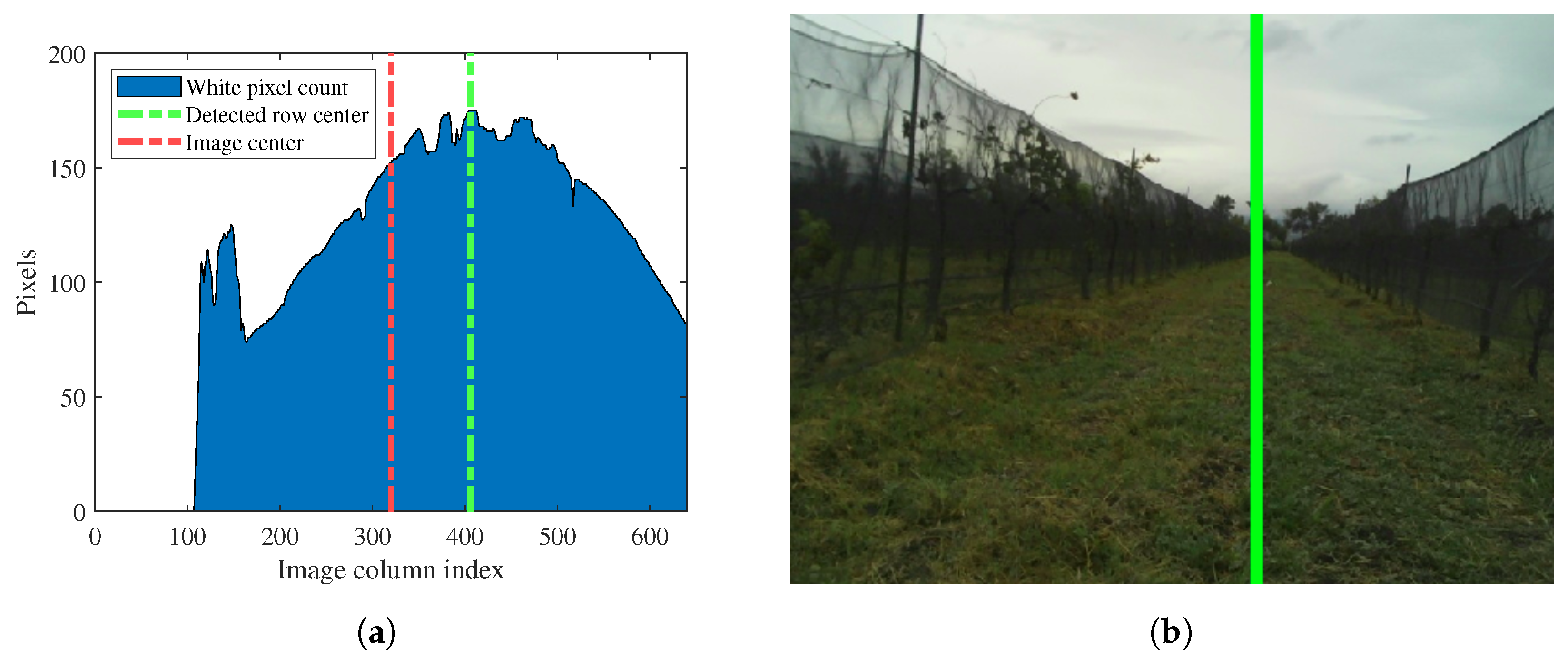
The mask containing the largest blob resembles a parabolic curve, with the vertex representing the middle of the row. To find the position of the row’s center in the image, the vertex must be determined.
To locate the vertex, the image is analyzed by separating the pixels into columns. The values of each column are summed, as shown in (6), where the white pixels have a value of 1 and the black pixels have a value of 0. Here, represents the value of the pixel at coordinates in the image, and n is the number of pixels in each column of the image (480 for the camera used in this work). The sum of pixels in column j is denoted as .
After summing the values of each column separately and grouping them in an array as in (7) where m is the number of columns in the image, which is 640 for the camera used in this work. The column with the highest value is where the vertex is located using the max function for the array S. Therefore, the column c is identified as the column where the center of the row is located.
Furthermore, to reduce noise in the detection of the center of the row, instead of using c as the center, the mean of the 5 column index with the highest white pixel count is defined as the center of the detected row.
3.5. Navigation
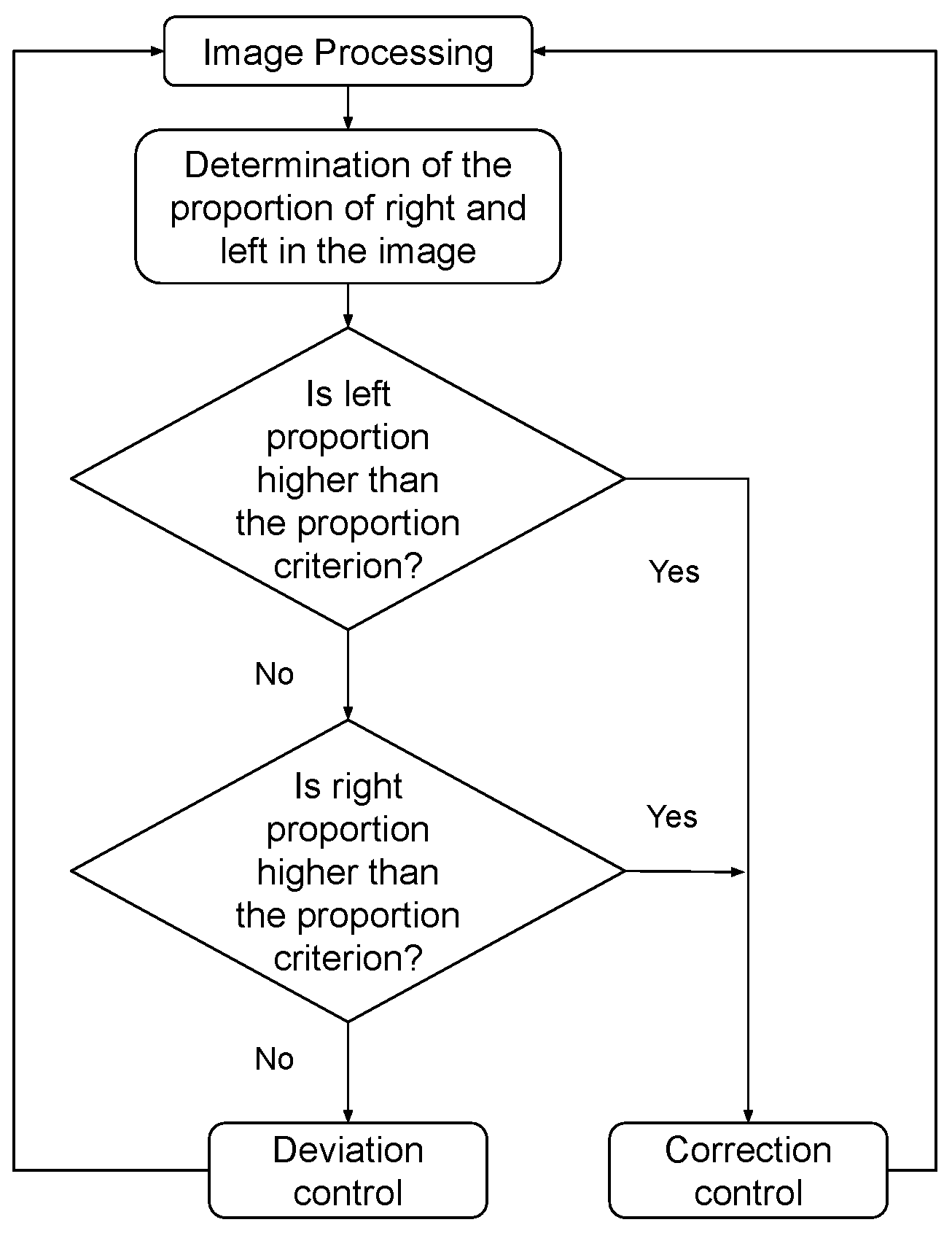
The algorithm uses a commutable control system to navigate based on the information obtained from the image processing. Navigation control operates as a state machine with two distinct states: deviation control and correction control. This state machine determines the required angular velocity () to position the robot in the center of the row, while the linear velocity (V) remains constant.
Each control consists of a proportional gain multiplied by the calculated error. Correction control is responsible for guiding the robot towards the center of the row. It takes control when the proportion of white pixels on the right or left side of the crop row exceeds a predefined criterion (explained in Section 3.5.1). On the other hand, the deviation control allows the robot to rotate towards the front of the row. It takes control when the conditions for the correction control are not met. The logic of the state machine is illustrated in Figure 9.
3.5.1. Correction Control Mode
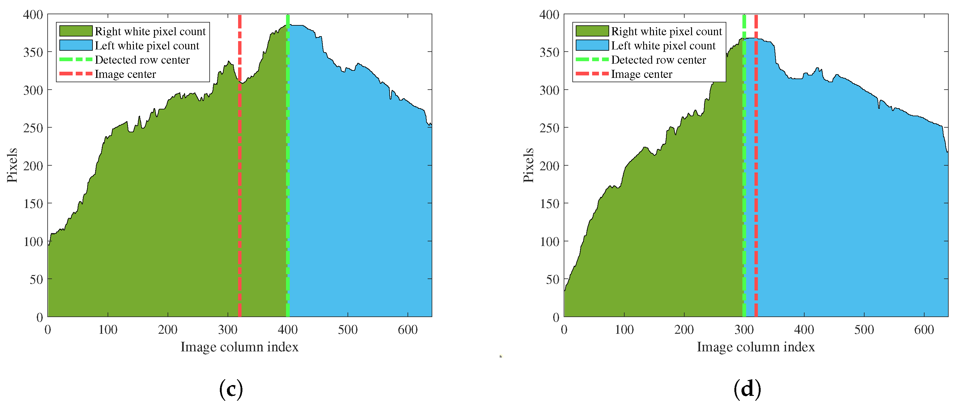
In this mode, the algorithm calculates the number of white pixels on the right and left sides of the image using (9). It considers the center of the row calculated by the image processing algorithm, rather than the center of the entire image. Once the number of white pixels on each side is determined, the proportion of white pixels on one side relative to the other side is calculated. If the vineyard is symmetric and the robot is well-centered, this proportion should be 1. However, when this proportion exceeds a predefined value, the proportional criterion (); it is considered the system error (E).
Note that for unsymetrical landscapes the should be greater or determined in trials.
The error (E) is then used to calculate the required angular velocity () for error correction. This is achieved using static-state feedback (P) in (10).
For example, in both Figure 10a,b, the robot is situated on the left side of the row, indicating that it needs to turn right to move towards the center. The difference lies in the proximity to the center of the row: in Figure 10a, the robot is close to the row center, and the deviation mode alone is sufficient to correct the error. However, in Figure 10b, the robot is located near the border of the left row, and the white pixel distribution suggests that the robot is already at the center or, as in this case, should turn left, since the detected row center is to the left of the image center. In this scenario, the deviation mode would exacerbate the error and would fail to guide the robot to the center of the row. Hence, the correction mode is activated because, as seen in Figure 10d, , exceeding the predefined value of 1.5 in this work. Therefore, the deviation mode instructs the robot to turn right, regardless of the detected location of the row center, ultimately leading the robot to the center of the row.
3.5.2. Deviation Control Mode
This control calculates the deviation (D) of the center of the row (C), determined by image processing, from the center of the image (Equation (11)). The deviation is then used in (12) to calculate the angular velocity required to correct the deviation, where G represents the proportional gain of this control. The proportional control is used instead of a PD or PID control due to its simplicity, as the latter controls can introduce additional noise in the output, which is not recommended for this type of application where input signal have a lot of variations. No perceptible stationary error was found during the testing and, therefore, no PI controller was not used.
3.5.3. Tuning
As the navigation constantly switches between both controls, there are three values that need to be adjusted. For the deviation control mode, there is the deviation gain, and for the correction mode, there are the proportional criterion and the correction gain. When running the test for tuning, the user must try to obtain gain values that allow the change of angular velocity to be small when a switch of controls occurs. The proportional criterion must be greater than 1 in order for the deviation control mode to work. It is important to note that the higher the proportional criterion, the more dominant the deviation mode in navigation. This adjustment is made manually.
3.6. Experimental Setup
To evaluate the performance of the algorithm, tests were carried out with five different initial conditions, as shown in Figure 11. These initial conditions were selected to assess the system’s ability to correct various types of errors. The first initial condition represents the robot being perfectly centered and heading towards the front. The second and third initial conditions involve the robot being centered in the vineyard but heading to the left and right, respectively, requiring the control to correct the robot’s orientation. The last two initial conditions involve the robot heading towards the front while positioned on the left and right sides of the vineyard.
After placing the robot in an initial condition, the algorithm was tested for a short period of time. As the proposed system is meant to be a backup plan the idea was to make sure the system was able to correct quickly, so the execution of each test was of ten seconds to evaluate its performance.
The control parameters shown in Table 1 were used for the test; they were found in trials using the method described in Section 3.5.3:
Validation Node
To track the performance of the algorithm, a ROS node was set up to record the deviation from the right and left sides of the vineyard row. A LiDAR sensor, model A3 manufactured by Slamtec (Shanghi, China), was used to measure the distances from the sides, although it was not utilized during the navigation process. The recorded data was then used to generate graphs (Figure 12) to analyze how well the robot followed the track. These graphs illustrate the centering error over the course of navigation, enabling visualization of the corrections made by the navigation system.
Since the LiDAR cannot detect the tree rows or the net in the vineyard due to existing spaces, Kraft paper was placed in the lower part of the net (as shown in Figure 11) to allow the LiDAR to detect distances accurately. The image processing algorithm was tested both with and without Kraft paper, and it was found that the paper had no impact on the resulting images obtained from image processing.
4. Results
Two tests were performed for each initial condition defined in Section 3.6 to analyze the robot’s performance. Both tests had similar results, the graphs in Figure 12 show the representative results. The validation node recorded the deviation from the right and left sides of the vineyard row, which was used to generate graphs illustrating the robot’s error. These graphs represent the difference between the distances detected by the LiDAR sensor on the left and right sides, with zero indicating the robot’s centered position, negative numbers indicating deviation to the left, and positive numbers indicating deviation to the right.
The recorded data generated graphs (Figure 12) displaying the centering error over the course of navigation, providing a visualization of the corrections made by the navigation system.
The experiment aimed to achieve small errors, ensuring that the robot would not collide with the lane boundaries. An error less than 15% of the lane width was considered desirable.
In the first initial condition, the robot started the navigation centered in the lane. Despite a small deviation to the left caused by the movement of the vineyard mesh, due to air blowing the net that covers the vine trees, introducing noise in the LiDAR measurements; the robot physically started in a centered position. The resulting graph (Figure 12a) demonstrates the algorithm’s ability to maintain a relatively stable route when the robot is already on the correct track.
The second initial condition tested the algorithm’s performance when the robot was centered but rotated heading to the left. Diagram (Figure 12b) shows that the robot’s path had more oscillations compared to when the robot was centered and heading forward. This indicates constant changes in the navigation control gains to correct the robot’s orientation and align it with the forward direction.
The third initial condition aimed to test the algorithm’s performance when the robot was centered but rotated heading to the right. Since the only difference between the second and third initial conditions was the orientation side, similar behavior was expected in both tests. The error line in Figure 12c exhibits oscillations similar to the second test, but in this case, the robot corrected its orientation more quickly and maintained a more centered navigation along the lane.
In the fourth initial condition, the robot was positioned at the left side of the lane, heading forward. The objective of this test was to evaluate whether the algorithm could correct the navigation and drive the robot to the center of the lane. The graph in Figure 12d shows a consistent decrease in the error, approaching the center of the lane by the end of the navigation. The resulting path is not a straight line to the center, as environmental noise introduced into the system affects the robot’s movement.
The fifth initial condition placed the robot on the right side of the lane, heading forward. The expected behavior was a similar navigation to the previous test, but with a decreasing error from the right side. The graph in Figure 12e shows a constant decrease in error, directing the robot towards the center. However, in this test, the robot did not get as close to the center as in the previous test, which is attributed to differences in ground on each side of the lane due to the irregular soil row.
As can be seen in the graphs, regardless of the initial condition, the tests demonstrate that the algorithm was able to decrease the centering error. The robot never reached the exact center, but it remained constant in proximity to it. In Figure 12a, when the robot started in a centered position, the navigation error remained below 30 cm. In Figure 12b,c, when the robot started with a rotation, the correction initially caused the robot to deviate to the opposite side but quickly corrected its path after a few seconds. In Figure 12d,e, when the robot started on the sides, the algorithm constantly corrected the path towards the center. The navigation behavior using the proposed algorithm demonstrates its ability to correct deviations along the robot’s path. These results indicate that the algorithm can effectively drive the robot through a vineyard in the forward direction without colliding, making it suitable for agricultural applications.
Efficiency
One way to evaluate the efficiency of a computational algorithm is to calculate its time complexity. For this work to calculate the complexity of the algorithm, each step is individually analyzed, as shown in Figure 4. First, the image is converted to grayscale, which involves iterating through each pixel and applying the grayscale transformation. This step has a time complexity of , where n represents the height of the image and m the width. Next, a Gaussian blur is applied to the grayscale image, which also requires processing each pixel with a Gaussian kernel. The time complexity of this operation is also .
The Otsu’s thresholding technique is then applied to the blurred image. Otsu’s thresholding calculates the optimal threshold value to separate foreground and background pixels in the grayscale image. Like the previous steps, this operation has a time complexity of .
Blob detection is achieved by using contour detection. This operation analyzes the pixels in the image to identify contours. It has a time complexity of . The creation of the mask with the biggest blob involves initializing a matrix of zeros with the same dimensions as the image and converting it to the ‘uint8’ data type. This process has a complexity of . Additionally, filling the mask with the maximum contour requires operations, where b corresponds to the number of points in the contour. Therefore, the overall complexity of mask creation is .
Finally, the algorithm proceeds to calculate the column sums of the processed image. This step involves adding the pixel values for each column in the image. The time complexity of this operation is proportional to the number of columns equal to the width of the image. The column sums are then sorted and the index of the highest sum is calculated. The classification of n elements has a time complexity of . Index calculation is a constant-time operation.
Taking into account all the steps involved, the time complexity can be approximated to the more complex process in the algorithm. This means that the algorithm has a time complexity of , where represents the number of pixels in the image and b is the number of pixels in the contour of the largest detected blob.
Comparing the algorithm complexity achieved with the backup method presented by Aghi [20], demonstrate the advantage of our solution. The backup method presented in the literature uses a CNN with an overall depth of 90 layers and with 3,492,035 parameters. The literature does not provide a way to calculate its complexity however a CNN model of this characteristics is more complex than the solution presented. Since this research avoids the use of a neural network it also avoids the model training and instead is needed a tuning process. The tuning is easier to set because there is no need for a data set of images or pre-processing. In addition, the computational cost is less since the number of adjusted parameters is significantively minor. For example, four parameters should change in the presented solution against 3,492,035 parameters in Aghi’s [20].
5. Conclusions
In this work, we proposed an algorithm to navigate a vineyard row using a low-cost 2D camera and Otsu’s thresholding. Unlike machine learning-based techniques, this algorithm does not require prior training and only needs to be tuned.
Two control methods were implemented to correct the robot position error in the vineyard row. The first method determines the center of the row by identifying the region in the image with the most background, considering that the background corresponds to the most distant objects. The second method maintains a proportional amount of background on the left and right sides of the image.
During testing, Otsu’s thresholding successfully separates the bottom of the vine row, allowing the correct centered navigation. Unlike other works that use Otsu’s method, this work does not utilize the Hough transform to identify crop lines, thus reducing the complexity and computational resources needed.
Experimental trials demonstrated the ability of the algorithm to guide the robot to the center of the row and allow it to navigate the row without collisions. The algorithm effectively directed the robot to the center even when it initially faced one of the row walls or was not positioned at the center, accomplishing this in a short time lapse of 10 s, all of which are necessary features for a backup navigation system.
Since the algorithm does not require prior training and has a lower time complexity compared to CNN, this autonomous navigation method of navigation serves as an alternative to the state-of-the-art secondary navigation systems. Additionally, this algorithm is resilient to light variations and can be used in any growth stage because of the dynamic thresholding used to identify the background.
However this work has limitations since it has been only tested in vineyards rows that utilize a net to protect the fruits, additionally this algorithm is intended to work only in straight rows and is not capable of avoiding obstacles present in the path.
For future work, this algorithm can be applied to other similar scenarios, such as other agricultural fields or hall-like structures. Additionally, there are plans to implement this methodology on a larger robotic platform to test its performance on uneven terrains.
Author Contributions
Conceptualization, E.M., J.P.C., J.A.E.C. and A.G.-E.; Methodology, E.M., J.P.C., J.A.E.C. and A.G.-E.; Software, E.M. and J.P.C.; Validation, E.M. and J.P.C.; Formal Analysis, E.M. and J.P.C.; Investigation, E.M. and J.P.C.; Writing—Original Draft Preparation, E.M. and J.P.C.; Writing—Review & Editing, E.M., J.P.C., J.A.E.C. and A.G.-E.; Visualization, E.M. and J.P.C.; Supervision, J.A.E.C. and A.G; Project Administration, E.M., J.P.C., J.A.E.C. and A.G.-E.; Resources J.A.E.C.; Funding A.G.-E. All authors have read and agreed to the published version of the manuscript.
Funding
This research received no external funding.
Data Availability Statement
The data presented in this study are available on request from the corresponding author.
Conflicts of Interest
The authors declare no conflict of interest.
References
- United Nations. World Population Is Expected to Reach 9.7 Billion in 2050 and Could Peak at Nearly 11 Billion around 2100; United Nations: San Francisco, CA, USA, 2019. [Google Scholar]
- Wang, T.; Chen, B.; Zhang, Z.; Li, H.; Zhang, M. Applications of machine vision in agricultural robot navigation: A review. Comput. Electron. Agric. 2022, 198, 107085. [Google Scholar] [CrossRef]
- Jararweh, Y.; Fatima, S.; Jarrah, M.; AlZu’bi, S. Smart and sustainable agriculture: Fundamentals, enabling technologies, and future directions. Comput. Electr. Eng. 2023, 110, 108799. [Google Scholar] [CrossRef]
- Kanagasingham, S.; Ekpanyapong, M.; Chaihan, R. Integrating machine vision-based row guidance with GPS and compass-based routing to achieve autonomous navigation for a rice field weeding robot. Precis. Agric. 2020, 21, 831–855. [Google Scholar] [CrossRef]
- Nehme, H.; Aubry, C.; Solatges, T.; Savatier, X.; Rossi, R.; Boutteau, R. LiDAR-based Structure Tracking for Agricultural Robots: Application to Autonomous Navigation in Vineyards. J. Intell. Robot. Syst. Theory Appl. 2021, 103, 61. [Google Scholar] [CrossRef]
- Bonadies, S.; Gadsden, S.A. An overview of autonomous crop row navigation strategies for unmanned ground vehicles. Eng. Agric. Environ. Food 2019, 12, 24–31. [Google Scholar] [CrossRef]
- Ji, R.; Qi, L. Crop-row detection algorithm based on Random Hough Transformation. Math. Comput. Model. 2011, 54, 1016–1020. [Google Scholar] [CrossRef]
- Liang, X.; Chen, B.; Wei, C.; Zhang, X. Inter-row navigation line detection for cotton with broken rows. Plant Methods 2022, 18, 90. [Google Scholar] [CrossRef]
- Li, X.; Lloyd, R.; Ward, S.; Cox, J.; Coutts, S.; Fox, C. Robotic crop row tracking around weeds using cereal-specific features. Comput. Electron. Agric. 2022, 197, 106941. [Google Scholar] [CrossRef]
- Vidović, I.; Cupec, R.; Hocenski, Ž. Crop row detection by global energy minimization. Pattern Recognit. 2016, 55, 68–86. [Google Scholar] [CrossRef]
- Guerrero, J.M.; Ruz, J.J.; Pajares, G. Crop rows and weeds detection in maize fields applying a computer vision system based on geometry. Comput. Electron. Agric. 2017, 142, 461–472. [Google Scholar] [CrossRef]
- Alagbo, O.; Spaeth, M.; Saile, M.; Schumacher, M.; Gerhards, R. Weed Management in Ridge Tillage Systems—A Review. Agronomy 2022, 12, 910. [Google Scholar] [CrossRef]
- Ma, Z.; Yin, C.; Du, X.; Zhao, L.; Lin, L.; Zhang, G.; Wu, C. Rice row tracking control of crawler tractor based on the satellite and visual integrated navigation. Comput. Electron. Agric. 2022, 197, 106935. [Google Scholar] [CrossRef]
- Shi, J.; Bai, Y.; Diao, Z.; Zhou, J.; Yao, X.; Zhang, B. Row Detection BASED Navigation and Guidance for Agricultural Robots and Autonomous Vehicles in Row-Crop Fields: Methods and Applications. Agronomy 2023, 13, 1780. [Google Scholar] [CrossRef]
- Benson, E.R.; Reid, J.F.; Zhang, Q. Machine vision-based guidance system for an agricultural small-grain harvester. Trans. ASAE 2023, 46, 1255. [Google Scholar] [CrossRef]
- Otsu, N. Threshold selection method from gray-level histograms. IEEE Trans. Syst. Man Cybern. 1979, SMC-9, 62–66. [Google Scholar] [CrossRef]
- Ravankar, A.; Ravankar, A.A.; Watanabe, M.; Hoshino, Y.; Rawankar, A. Development of a low-cost semantic monitoring system for vineyards using autonomous robots. Agriculture 2020, 10, 182. [Google Scholar] [CrossRef]
- Zheng, S.; Wang, J.; Rizos, C.; Ding, W.; El-Mowafy, A. Simultaneous Localization and Mapping (SLAM) for Autonomous Driving: Concept and Analysis. Remote Sens. 2023, 15, 1156. [Google Scholar] [CrossRef]
- Astolfi, P.; Gabrielli, A.; Bascetta, L.; Matteucci, M. Vineyard Autonomous Navigation in the Echord++ GRAPE Experiment. IFAC-PapersOnLine 2018, 51, 704–709. [Google Scholar] [CrossRef]
- Aghi, D.; Mazzia, V.; Chiaberge, M. Local motion planner for autonomous navigation in vineyards with a RGB-D camera-based algorithm and deep learning synergy. Machines 2020, 8, 27. [Google Scholar] [CrossRef]
- Ronchetti, G.; Mayer, A.; Facchi, A.; Ortuani, B.; Sona, G. Crop row detection through UAV surveys to optimize on-farm irrigation management. Remote Sens. 2020, 12, 1967. [Google Scholar] [CrossRef]
- Berenstein, R.; Shahar, O.B.; Shapiro, A.; Edan, Y. Grape clusters and foliage detection algorithms for autonomous selective vineyard sprayer. Intell. Serv. Robot. 2010, 3, 233–243. [Google Scholar] [CrossRef]
- Chen, J.; Qiang, H.; Wu, J.; Xu, G.; Wang, Z. Navigation path extraction for greenhouse cucumber-picking robots using the prediction-point Hough transform. Comput. Electron. Agric. 2021, 180, 105911. [Google Scholar] [CrossRef]
- Dogru, S.; Marques, L. An improved kinematic model for skid-steered wheeled platforms. Auton. Robot. 2021, 45, 229–243. [Google Scholar] [CrossRef]
- ROS Wiki. Documentation. 2021. Available online: http://wiki.ros.org/Documentation (accessed on 5 May 2023).
Figure 1.
Skid steering mobile robot kinematic diagram. Where and represent a plane surface with an inertial orthonormal basis; X and Y, is the local coordinate frame with respect to a inertial frame; b is the vehicle width; a is the vehicle length; G is the center of mass; is the point of rotation; , is the local coordinate frame assigned to the robot at its center of mass; , is the displacement of from G; shows the instantaneous Center of Rotation; represents longitudinal velocity and is the lateral velocity.

Figure 2.
Vineyard.

Figure 3.
Robotic platform: (1) Camera, (2) LiDAR (for performance measurement), (3) Laptop, (4) Skid Steering Mobile Robot.
Figure 3.
Robotic platform: (1) Camera, (2) LiDAR (for performance measurement), (3) Laptop, (4) Skid Steering Mobile Robot.

Figure 4.
Visual diagram of the visual processing method described in this paper based on three sections for center identification of the row. Asymptotic complexity marked in red, where n is the number of rows in the image, m is the number of columns and b is the number of pixels of the contour of the biggest blob.

Figure 5.
Image changes during processing. (a) Original image taken by the camera. (b) Image transformed to gray scale values. (c) Segmented image using the Otsu’s method.
Figure 5.
Image changes during processing. (a) Original image taken by the camera. (b) Image transformed to gray scale values. (c) Segmented image using the Otsu’s method.

Figure 6.
Identification of the largest blob eliminates noise from the image as shown in this Figure.
Figure 6.
Identification of the largest blob eliminates noise from the image as shown in this Figure.

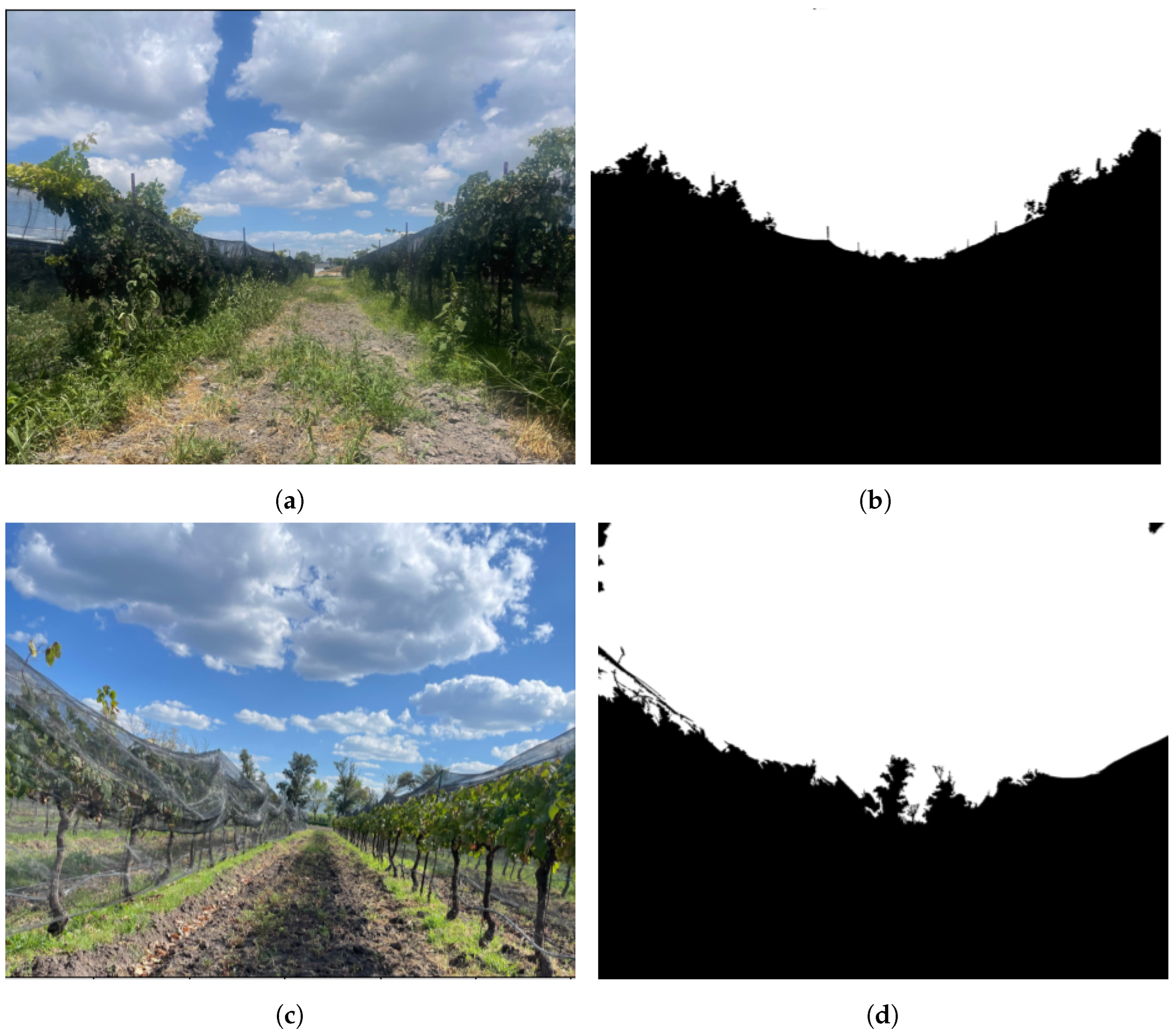
Figure 7.
Image processing at different conditions. (a) Sunny day with clouds presence and weed in the path. (b) Biggest blob’s mask of Figure 7a. (c) Sunny day with trees at the background and a shadow in the path. (d) Biggest blob’s mask of Figure 7c.

Figure 8.
Row center detection. (a) Pixel count analysis area graph. (b) A green line is drawn where the center of the row was detected over the original vineyard image.
Figure 8.
Row center detection. (a) Pixel count analysis area graph. (b) A green line is drawn where the center of the row was detected over the original vineyard image.

Figure 9.
Commutable control logic.

Figure 10.
Correction mode pixel count. (a) Image when the robot is near the row center. (b) Image when the robot is near the row border. (c) Pixel count analysis of Figure 10a. (d) Pixel count analysis of Figure 10b.


Figure 11.
Initial conditions. (a) In the center and heading to the front. (b) In the center and heading to the left. (c) In the center heading to the right. (d) At the left and heading to the front. (e) At the right and heading to the front.
Figure 11.
Initial conditions. (a) In the center and heading to the front. (b) In the center and heading to the left. (c) In the center heading to the right. (d) At the left and heading to the front. (e) At the right and heading to the front.

Figure 12.
Results graphs. (a) Initial condition 1 test. (b) Initial condition 2 test. (c) Initial condition 3 test. (d) Initial condition 4 test. (e) Initial condition 5 test.
Figure 12.
Results graphs. (a) Initial condition 1 test. (b) Initial condition 2 test. (c) Initial condition 3 test. (d) Initial condition 4 test. (e) Initial condition 5 test.


Table 1.
Control parameters used on the tests.
| Variable | Value |
|---|---|
| V | |
| G | |
| P | |
Disclaimer/Publisher’s Note: The statements, opinions and data contained in all publications are solely those of the individual author(s) and contributor(s) and not of MDPI and/or the editor(s). MDPI and/or the editor(s) disclaim responsibility for any injury to people or property resulting from any ideas, methods, instructions or products referred to in the content. |
© 2023 by the authors. Licensee MDPI, Basel, Switzerland. This article is an open access article distributed under the terms and conditions of the Creative Commons Attribution (CC BY) license (https://creativecommons.org/licenses/by/4.0/).
Share and Cite
MDPI and ACS Style
Mendez, E.; Piña Camacho, J.; Escobedo Cabello, J.A.; Gómez-Espinosa, A. Autonomous Navigation and Crop Row Detection in Vineyards Using Machine Vision with 2D Camera. Automation 2023, 4, 309-326. https://doi.org/10.3390/automation4040018
AMA Style
Mendez E, Piña Camacho J, Escobedo Cabello JA, Gómez-Espinosa A. Autonomous Navigation and Crop Row Detection in Vineyards Using Machine Vision with 2D Camera. Automation. 2023; 4(4):309-326. https://doi.org/10.3390/automation4040018
Chicago/Turabian StyleMendez, Enrico, Javier Piña Camacho, Jesús Arturo Escobedo Cabello, and Alfonso Gómez-Espinosa. 2023. "Autonomous Navigation and Crop Row Detection in Vineyards Using Machine Vision with 2D Camera" Automation 4, no. 4: 309-326. https://doi.org/10.3390/automation4040018