Cost Function Approach for Dynamical Component Analysis: Full Recovery of Mixing and State Matrix

Abstract

A reformulation of the dynamical component analysis (DyCA) via an optimization-free approach is presented. The original cost function approach is converted into a numerical linear algebra problem, i.e., the computation of coupled singular-value decompositions. A simple algorithm is presented together with numerical experiments to document the feasability of the approach. This methodology is able to recover the mixing and state matrices of multivariate signals from high-dimensional measured data fully.

1. Introduction

An important task in signal processing is the decomposition of a multivariate signal for the analysis of measured or simulated data leading to the possible detection of the relevant subspace or the sources of the signal. Recently, a new method—dynamical component analysis (DyCA)—based on modeling the signal via two coupled systems of ordinary differential equations (ODE) was introduced. One system is governed by time-invariant linear dynamics, whereas the second one is defined by an unknown non-linear vector field, assumed to be smooth. Its derivation and its features have been presented in depth (see [1,2]). The presented algorithm was nearly as simple as principal component analysis (PCA) or certain independent component analysis (ICA) approaches. The results obtained via DyCA, however, yield deeper insight into the underlying dynamics of the data. Moreover, as demonstrated by several examples in [2], typically, neither ICA nor PCA approaches are able to capture the linear/non-linear character of the underlying dynamics.

The present work, in particular, is partially based on two conference papers [3,4]. Moreover, our objective is to reformulate the original cost function approach for DyCA— formerly leading to a generalized eigenvalue, or more generally, to an invariant eigenspace problem—into an inverse-problem-type formulation, which allows for the recovery of the state and mixing matrices from high-dimensional matrix-valued time series.

This paper is organized as follows. First, the general problem is briefly reviewed; the cost function is discussed in detail; and, in particular, the critical points are analyzed. Second, we formulate an optimization-free algorithm, mainly based on solving coupled singular-value decompositions. Finally, we present numerical experiments to support our approach.

2. Problem Formulation

Consider a signal $Q=[q\left(t_1\right),\dots ,q\left(t_T\right)]\in {\mathbb{R}}^{N\times T}$ and its derivative with respect to time denoted by $\dot{Q}\in {\mathbb{R}}^{N\times T}$.

Let $1\le m\le n\le N$. Assume that Q and $\dot{Q}$ are of the form

$$\begin{array}{cc}\hfill Q& =WX,\hfill \\ \hfill \dot{Q}& =W\dot{X},\hfill \end{array}$$

(1)

where $W\in {\mathbb{R}}^{N\times n}$ is a constant matrix of rank $n=\mathrm{rank}\left(W\right)$ and $X=[x\left(t_1\right),\dots ,x\left(t_T\right)],\dot{X}=[\dot{x}\left(t_1\right),\dots ,\dot{x}\left(t_T\right)]\in {\mathbb{R}}^{N\times T}$ are samples of $x:[t_1,t_T]\to {\mathbb{R}}^n$, fulfilling the ODE

$$\begin{array}{cc}\hfill [I_m,0]\dot{x}\left(t\right)& =Ax\left(t\right),\hfill \\ \hfill [0,I_{n-m}]\dot{x}\left(t\right)& =f\left(x\right(t\left)\right).\hfill \end{array}$$

(2)

Here, $A\in {\mathbb{R}}^{m\times n}$ is some constant matrix and $f:{\mathbb{R}}^n\to {\mathbb{R}}^{n-m}$ is an unknown smooth function. Under these assumptions, we formulate the problem that will be addressed in the sequel.

Problem 1

(DyCA).  

• Given a signal $Q\in {\mathbb{R}}^{N\times T}$, its derivative $\dot{Q}\in {\mathbb{R}}^{N\times T}$ with $1\le m\le n\le N$.
• Find estimates in a least squares sense for $A\in {\mathbb{R}}^{m\times n}$, $W\in {\mathbb{R}}^{N\times n}$, and $X,\dot{X}\in {\mathbb{R}}^{N\times T}$ according to the above assumptions.

Defining $f\left(X\right):=[f\left(x_1\right),\dots ,f\left(x_T\right)]\in {\mathbb{R}}^{n\times T}$, we obtain the following via Equations (1) and (2):

$$\begin{array}{cc}\hfill Q& =WX,\hfill \\ \hfill \dot{Q}& =W\left[\begin{array}{c}AX\\ f\left(X\right)\end{array}\right].\hfill \end{array}$$

(3)

We will propose a method by which to solve Problem 1, assuming exact data.

3. Cost Function

We approach the DyCA problem by minimizing a suitable cost function. Similar to [5], we fit the part of the data corresponding to the linear part of the ODE by minimizing the cost:

$$\begin{array}{cc}\hfill f:{\mathbb{R}}^{N\times n}\times {\mathbb{R}}^{m\times n}& \to \mathbb{R},\hfill \\ \hfill (W,A)& \mapsto \parallel [I_m,0]\dot{X}-AX{\parallel }_F^2.\hfill \end{array}$$

(4)

Here, X and $\dot{X}$ depend implicitly on W.

To derive a more explicit expression for Equation (4), we rewrite Equation (3) by considering thin singular-value decompositions (SVDs) of Q and $\dot{Q}$, respectively. In more detail, let

$${\theta }_0{\Sigma }_0{\Xi }_0^{\top }=Q\stackrel{\left(3\right)}{=}WX$$

(5)

be a thin SVD of Q, where ${\theta }_0\in {\mathrm{St}}_{N,n}$, ${\Sigma }_0\in {\mathbb{R}}^{n\times n}$ diagonal and ${\Xi }_0\in {\mathrm{St}}_{T,n}$. Analogously, let

$$\begin{array}{cc}\hfill {\theta }_2{\Sigma }_2{\Xi }_2^{\top }& =\dot{Q}\hfill \\ & \stackrel{\left(3\right)}{=}W\left[\begin{array}{c}AX\\ f\left(X\right)\end{array}\right]\hfill \end{array}$$

(6)

be a thin SVD of $\dot{Q}$, where ${\theta }_2\in {\mathrm{St}}_{N,n}$, ${\Sigma }_0\in {\mathbb{R}}^{n\times n}$ diagonal and ${\Xi }_2\in {\mathrm{St}}_{T,n}$. As usual, (cf., e.g., [4]), the Stiefel manifold is denoted by

$${\mathrm{St}}_{a,b}:=\{X\in {\mathbb{R}}^{a\times b}\mid X^{\top }X=I_b\},$$

(7)

i.e., a differentiable submanifold of the vector space ${\mathbb{R}}^{a\times b}$ with $a\ge b$ consisting of rectangular matrices with orthonormal columns. Exploiting ${\theta }_i^{\top }{\theta }_i=I_k$ for $i\in \{0,2\}$, we obtain via Equation (5):

$$\left({\theta }_0^{\top }W\right)X={\Sigma }_0{\Xi }_0^{\top },$$

(8)

while Equation (6) yields

$$\left({\theta }_2^{\top }W\right)\dot{X}={\Sigma }_2{\Xi }_2^{\top }.$$

(9)

For $i\in \{0,2\}$, we set

$$\begin{array}{cc}\hfill G_i& =G_i\left(W\right)\hfill \\ & =G_i({\theta }_i,W)\hfill \\ & :={\theta }_i^{\top }W\in {\mathbb{R}}^{n\times n}.\hfill \end{array}$$

(10)

Via the assumptions imposed in the formulation of the DyCA problem, we have for $i\in \{0,2\}$

$$\mathrm{span}\left(W\right)=\mathrm{span}\left({\theta }_i\right),$$

(11)

yielding $G_i={\theta }_i^{\top }W\in \mathrm{GL}\left(n\right)$; i.e., $G_i$ is invertible.

Hence, solving Equation (5), as well as Equation (6) for X and $\dot{X}$, respectively, and putting the result into Equation (4) yields the smooth cost

$$\begin{array}{cc}\hfill f:{\mathbb{R}}^{N\times n}\times {\mathbb{R}}^{m\times n}& \to \mathbb{R},\hfill \\ \hfill (W,A)& \mapsto f(W,A):=\parallel [I_m,0]G_2^{-1}{\Sigma }_2{\Xi }_2^{\top }-A{G}_0^{-1}{\Sigma }_0{\Xi }_0^{\top }{\parallel }_F^2,\hfill \end{array}$$

(12)

where $G_0=G_0\left(W\right)$ and $G_2=G_2\left(W\right)$ are given via Equation (10).

Remark 1.

Essentially, the cost function Equation (12) considered here is a reformulation of the one considered earlier (see [2,5] and several follow up papers, in particular, e.g., [3,6]). There is, however, an important difference; the reformulation here takes, in some sense, the inverse problem character explicitly into consideration.

Remark 2.

Strictly speaking, the cost f defined in Equation (12) is not defined on the whole space ${\mathbb{R}}^{N\times n}\times {\mathbb{R}}^{m\times n}$ but only on the subset given by $U\times {\mathbb{R}}^{m\times n}$, where

$$\begin{array}{cc}\hfill U& =\left\{W\in {\mathbb{R}}^{N\times n}\mid {\theta }_0^{\top }W\in \mathrm{GL}\left(n\right)\mathit{and}{\theta }_2^{\top }W\in \mathrm{GL}\left(n\right)\right\}\hfill \\ \hfill & ={\varphi }_0^{-1}\left(\mathbb{R}\setminus \left\{0\right\}\right)\cap {\varphi }_2^{-1}\left(\mathbb{R}\setminus \left\{0\right\}\right),\hfill \end{array}$$

(13)

where ${\varphi }_i:{\mathbb{R}}^{N\times n}\to \mathbb{R}$ are the continuous functions defined for $i\in \{0,2\}$ by

$${\varphi }_i\left(W\right)=det\left({\theta }_i^{\top }W\right).$$

(14)

Note that $U\subseteq {\mathbb{R}}^{N\times n}$ is open by the second equality in Equation (13) and the continuity of ${\varphi }_i$. Thus, the domain of f, namely, $U\times {\mathbb{R}}^{n\times m}$, is an open subset of ${\mathbb{R}}^{N\times n}\times {\mathbb{R}}^{n\times m}$.

Notation 1.

From now on, if not indicated otherwise, $U\times {\mathbb{R}}^{m\times n}\subseteq {\mathbb{R}}^{N\times n}\times {\mathbb{R}}^{m\times n}$ denotes the domain of f as characterized in Remark 2.

In the sequel, through abuse of notation, we sometimes write $f:{\mathbb{R}}^{N\times n}\times {\mathbb{R}}^{m\times n}\to \mathbb{R}$ instead of $f:U\times {\mathbb{R}}^{m\times n}\to \mathbb{R}$.

4. Analysis of the Cost

4.1. Derivatives

Obviously, $f:U\times {\mathbb{R}}^{m\times n}\to \mathbb{R}$ is a smooth function. To obtain candidates for points $(W,A)\in U\times {\mathbb{R}}^{m\times n}$, where f attains a minimum, we search for critical points of f.

As a preparation, to compute the derivative of f, we recall the following well-known lemma.

Lemma 1.

The derivative of

$$\begin{array}{cc}\hfill \mathrm{inv}:\mathrm{GL}\left(n\right)& \to \mathrm{GL}\left(n\right),\hfill \\ \hfill A& \mapsto \mathrm{inv}\left(A\right)=A^{-1},\hfill \end{array}$$

(15)

evaluated at $A\in \mathrm{GL}\left(n\right)$ in direction $B\in {\mathbb{R}}^{n\times n}$, is given by

$$\mathrm{D}\left(\mathrm{inv}\left(A\right)\right)B=-A^{-1}B{A}^{-1}.$$

(16)

Lemma 2.

Let $f:U\times {\mathbb{R}}^{m\times n}\to \mathbb{R}$ be defined via Equation (12) and set

$$\Xi ={\Xi }_2^{\top }{\Xi }_0\in {\mathbb{R}}^{n\times n}.$$

(17)

Moreover, let $(W,A)\in U\times {\mathbb{R}}^{m\times n}$ and $(w,a)\in {\mathbb{R}}^{N\times n}\times {\mathbb{R}}^{m\times n}$. Then, the derivative of $f(·,A):{\mathbb{R}}^{N\times n}\to \mathbb{R}$ at $W\in U$ in the direction $w\in {\mathbb{R}}^{N\times n}$ is given by

$$\begin{array}{cc}\hfill {\mathrm{D}}_{1}f(W,A)w& =-2\mathrm{tr}\left(G_2^{-1}{\theta }_2^{\top }w{G}_2^{-1}{\Sigma }_2^2{G}_2^{-T}\left[\begin{array}{ccc}{I}_m& & 0\\ 0& & 0\end{array}\right]\right)\hfill \\ \hfill & +2\mathrm{tr}\left(G_2^{-1}{\theta }_2^{\top }w{G}_2^{-1}{\Sigma }_2\Xi {\Sigma }_0{G}_0^{-\top }{A}^{\top }[I_m,0]\right)\hfill \\ \hfill & +2\mathrm{tr}\left(G_2^{-1}{\Sigma }_2\Xi {\Sigma }_0{G}_0^{-\top }{w}^{\top }{\theta }_0{G}_0^{-\top }{A}^{\top }[I_m,0]\right)\hfill \\ \hfill & -2\mathrm{tr}\left(G_0^{-1}{\theta }_0^{\top }w{G}_0^{-1}{\Sigma }_0^2{G}_0^{-\top }{A}^{\top }A\right),\hfill \end{array}$$

(18)

and the derivative of f with respect to the second argument, i.e., of the derivative of the function $f(W,·):{\mathbb{R}}^{m\times n}\to \mathbb{R}$ at $A\in {\mathbb{R}}^{m\times n}$ in the direction $a\in {\mathbb{R}}^{m\times n}$, reads

$${\mathrm{D}}_{2}f(W,A)a=-2\mathrm{tr}\left(G_2^{-1}{\Sigma }_2\Xi {\Sigma }_0{G}_0^{-\top }{a}^{\top }[I_m,0]\right)+2\mathrm{tr}\left(G_0^{-1}{\Sigma }_0^2{G}_0^{\top }{a}^{\top }A\right).$$

(19)

Proof. 

Expanding

$$\begin{array}{cc}\hfill f(W,A)& =\mathrm{tr}\left(G_2^{-1}{\Sigma }_2^2{G}_2^{-\top }\left[\begin{array}{ccc}{I}_m& & 0\\ 0& & 0\end{array}\right]\right)-2\mathrm{tr}\left(G_2^{-1}{\Sigma }_2{\Xi }_2^{\top }{\Xi }_0{\Sigma }_0{G}_0^{-\top }{A}^{\top }[I_m,0]\right)\hfill \\ \hfill & +\mathrm{tr}\left(G_0^{-1}{\Sigma }_0^2{G}_0^{\top }{A}^{\top }A\right)\hfill \end{array}$$

(20)

and using Lemma 1, we obtain Equations (18) and (19) via a tedious but straightforward calculation.    □

Using Lemma 2, we search for critical points of f. Obviously, $(W,A)\in U\times {\mathbb{R}}^{m\times n}$ is a critical point of f iff the following two conditions, i.e.,

$$\begin{array}{cc}\hfill {\mathrm{D}}_{1}f(W,A)w& =0,\hfill \\ \hfill {\mathrm{D}}_{2}f(W,A)a& =0,\hfill \end{array}$$

(21)

hold for all $w\in {\mathbb{R}}^{N\times n}$ and $a\in {\mathbb{R}}^{m\times n}$.

Via Equation (18), we obtain ${\mathrm{D}}_{1}f(W,A)w=0$ for all $w\in {\mathbb{R}}^{N\times n}$ iff

$$\begin{array}{cc}\hfill 0& =-G_2^{-1}{\Sigma }_2^{-1}{G}_2^{-\top }\left[\begin{array}{ccc}{I}_m& & 0\\ 0& & 0\end{array}\right]G_2^{-1}{\theta }_2^{\top }\hfill \\ \hfill & +G_2^{-1}{\Sigma }_2\Xi {\Sigma }_0{G}_0^{-\top }{A}^{\top }[I_m,0]G_2^{-1}{\theta }_2^{\top }\hfill \\ \hfill & +G_0^{-1}{\Sigma }_0{\Xi }^{\top }{\Sigma }_2{G}_2^{-\top }\left[\begin{array}{c}{I}_m\\ 0\end{array}\right]A{G}_0^{-1}{\theta }_0^{\top }\hfill \\ \hfill & -G_0^{-1}{\Sigma }_0^2{G}_0^{-\top }{A}^{\top }A{G}_0^{-1}{\theta }_0^{\top }\hfill \end{array}$$

(22)

is satisfied. Clearly, Equation (22) is equivalent to

$$\begin{array}{cc}\hfill & G_2^{-1}\left({\Sigma }_2\Xi {\Sigma }_0{G}_0^{-\top }{A}^{\top }[I_m,0]-{\Sigma }_2^2{G}_2^{-\top }\left[\begin{array}{ccc}{I}_m& & 0\\ 0& & 0\end{array}\right]\right)G_2^{-1}{\theta }_2^{\top }\hfill \\ \hfill & =G_0^{-1}\left({\Sigma }_0^2{G}_0^{-\top }{A}^{\top }A-{\Sigma }_0{\Xi }^{\top }{\Sigma }_2{G}_2^{-\top }\left[\begin{array}{c}{I}_m\\ 0\end{array}\right]A\right)G_0^{-1}{\theta }_0^{\top }.\hfill \end{array}$$

(23)

Similarly, we obtain via Equation (19) that ${\mathrm{D}}_{2}f(W,A)a=0$ is fulfilled for all $a\in {\mathbb{R}}^{m\times n}$ iff

$$A{G}_0^{-1}{\Sigma }_0^2{G}_0^{-\top }=[I_m,0]G_2^{-1}{\Sigma }_2\Xi {\Sigma }_0{G}_0^{-\top }$$

(24)

holds. Because $G_0,{\Sigma }_0\in \mathrm{GL}\left(n\right)$ are invertible, Equation (24) is equivalent to

$$A=[I_m,0]G_2^{-1}{\Sigma }_2\Xi {\Sigma }_0^{-1}{G}_0.$$

(25)

Moreover, Equation (25) implies

$$\begin{array}{cc}\hfill A^{\top }[I_m,0]& =G_0^{\top }{\Sigma }_0^{-1}{\Xi }^{\top }{\Sigma }_2{G}_2^{-\top }\left[\begin{array}{ccc}{I}_m& & 0\\ 0& & 0\end{array}\right],\hfill \\ \hfill \left[\begin{array}{c}{I}_m\\ 0\end{array}\right]A& =\left[\begin{array}{ccc}{I}_m& & 0\\ 0& & 0\end{array}\right]G_2^{-1}{\Sigma }_2\Xi {\Sigma }_0^{-1}{G}_0,\hfill \\ \hfill A^{\top }A& =G_0^{\top }{\Sigma }_0^{-1}{\Xi }^{\top }{\Sigma }_2{G}_2^{-\top }\left[\begin{array}{ccc}{I}_m& & 0\\ 0& & 0\end{array}\right]G_2^{-1}{\Sigma }_2\Xi {\Sigma }_0^{-1}{G}_0.\hfill \end{array}$$

(26)

Plugging Equation (26) into Equation (23) yields

$$\begin{array}{cc}\hfill & G_2^{-1}\left({\Sigma }_2\Xi {\Sigma }_0{G}_0^{-\top }\left(G_0^{\top }{\Sigma }_0^{-1}{\Xi }^{\top }{\Sigma }_2{G}_2^{-\top }\left[\begin{array}{ccc}{I}_m& & 0\\ 0& & 0\end{array}\right]\right)-{\Sigma }_2^2{G}_2^{-\top }\left[\begin{array}{ccc}{I}_m& & 0\\ 0& & 0\end{array}\right]\right)G_2^{-1}{\theta }_2^{\top }\hfill \\ \hfill & =G_0^{-1}({\Sigma }_0^2{G}_0^{-\top }\left(G_0^{\top }{\Sigma }_0^{-1}{\Xi }^{\top }{\Sigma }_2{G}_2^{-\top }\left[\begin{array}{ccc}{I}_m& & 0\\ 0& & 0\end{array}\right]G_2^{-1}{\Sigma }_2\Xi {\Sigma }_0^{-1}{G}_0\right)\hfill \\ \hfill & -{\Sigma }_0{\Xi }^{\top }{\Sigma }_2{G}_2^{-\top }\left(\left[\begin{array}{ccc}{I}_m& & 0\\ 0& & 0\end{array}\right]G_2^{-1}{\Sigma }_2\Xi {\Sigma }_0^{-1}{G}_0\right))G_0^{-1}{\theta }_0^{\top }\hfill \\ \hfill & =0,\hfill \end{array}$$

(27)

being equivalent to

$$\begin{array}{cc}\hfill & G_2^{-1}\left({\Sigma }_2\Xi {\Xi }^{\top }{\Sigma }_2{G}_2^{-\top }\left[\begin{array}{ccc}{I}_m& & 0\\ 0& & 0\end{array}\right]-{\Sigma }_2^2{G}_2^{-\top }\left[\begin{array}{ccc}{I}_m& & 0\\ 0& & 0\end{array}\right]\right)G_2^{-1}{\theta }_2^{\top }\hfill \\ \hfill & =G_2^{-1}{\Sigma }_2\left(\Xi {\Xi }^{\top }-I_n\right){\Sigma }_2{G}_2^{-\top }\left[\begin{array}{ccc}{I}_m& & 0\\ 0& & 0\end{array}\right]G_2^{-1}{\theta }_2^{\top }\hfill \\ \hfill & =0.\hfill \end{array}$$

(28)

Multiplying Equation (28) from the left by $G_2{\Sigma }_2^{-1}$, as well as from the right by ${\theta }_2{G}_2$, and using the orthonormality property ${\theta }_2^{\top }{\theta }_2=I_n$ yields

$$(\Xi {\Xi }^{\top }-I_n){\Sigma }_2{G}_2^{-\top }\left[\begin{array}{ccc}{I}_m& & 0\\ 0& & 0\end{array}\right]=0.$$

(29)

Conversely, assume that Equation (29) is satisfied; then, Equation (28) holds. Thus, Equation (28) is equivalent to Equation (29).

The above discussion is summarized in the next Theorem.

Theorem 1.

Let $(W,A)\in U\times {\mathbb{R}}^{m\times n}$. Then, $(W,A)$ is a critical point of $f:U\times {\mathbb{R}}^{m\times n}\to \mathbb{R}$, defined in Equation (12), iff the following two equalities, i.e.,

$$(\Xi {\Xi }^{\top }-I_n){\Sigma }_2{G}_2^{-\top }\left[\begin{array}{ccc}{I}_m& & 0\\ 0& & 0\end{array}\right]=0$$

(30)

and

$$A=[I_m,0]G_2^{-1}{\Sigma }_2\Xi {\Sigma }_0^{-1}{G}_0,$$

(31)

hold. Here, for convenience, we used $G_0:={\theta }_0^{\top }W$.

4.2. Critical Points

In this section, the critical points of the DyCA cost are determined by using the characterization of Theorem 1, i.e., we solve the equation

$$(\Xi {\Xi }^{\top }-I_n){\Sigma }_2{G}_2^{-\top }\left[\begin{array}{ccc}{I}_m& & 0\\ 0& & 0\end{array}\right]=0$$

(32)

for $G_2\in \mathrm{GL}\left(n\right)$. To this end, we define

$$U:=(\Xi {\Xi }^{\top }-I_n){\Sigma }_2.$$

(33)

Then, Equation (32) is equivalent to

$$U{G}_2^{-\top }\left[\begin{array}{ccc}{I}_m& & 0\\ 0& & 0\end{array}\right]=0.$$

(34)

Set $F=U{G}_2^{-\top }$ and partition $F=\left[\begin{array}{ccc}{F}_{11}& & F_{12}\\ F_{21}& & F_{22}\end{array}\right]$, where $F_{11}\in {\mathbb{R}}^{m\times m}$, $F_{12}\in {\mathbb{R}}^{m\times (n-m)}$, $F_{21}\in {\mathbb{R}}^{(m-n)\times m}$, and $F_{22}\in {\mathbb{R}}^{(n-m)\times (n-m)}$. Then, Equation (34) yields

$$\begin{array}{cc}\hfill \left[\begin{array}{ccc}{F}_{11}& & F_{12}\\ F_{21}& & F_{22}\end{array}\right]\left[\begin{array}{ccc}{I}_m& & 0\\ 0& & 0\end{array}\right]& =\left[\begin{array}{ccc}{F}_{11}& & 0\\ F_{21}& & 0\end{array}\right]\hfill \\ \hfill & =0,\hfill \end{array}$$

(35)

i.e., Equation (34) holds iff $U{G}_2^{-\top }=\left[\begin{array}{ccc}0& & F_{12}\\ 0& & F_{22}\end{array}\right]$ is fulfilled. Next, partition

$$\begin{array}{cc}\hfill U& =\left[\begin{array}{ccc}{U}_{11}& & U_{12}\\ U_{21}& & U_{22}\end{array}\right],\hfill \\ \hfill G_2^{-\top }& =\left[\begin{array}{ccc}{\tilde{G}}_{11}& & {\tilde{G}}_{12}\\ {\tilde{G}}_{21}& & {\tilde{G}}_{22}\end{array}\right],\hfill \end{array}$$

(36)

where

$$\begin{array}{cc}\hfill U_{11},{\tilde{G}}_{11}& \in {\mathbb{R}}^{m\times m},\hfill \\ \hfill U_{21},{\tilde{G}}_{21}& \in {\mathbb{R}}^{(n-m)\times m},\hfill \\ \hfill U_{12},{\tilde{G}}_{12}& \in {\mathbb{R}}^{m\times (n-m)},\hfill \\ \hfill U_{22},{\tilde{G}}_{22}& \in {\mathbb{R}}^{(n-m)\times (n-m)},\hfill \end{array}$$

(37)

and consider

$$\begin{array}{cc}\hfill F& =U{G}_2^{-\top }\hfill \\ & =\left[\begin{array}{ccc}{U}_{11}& & U_{12}\\ U_{21}& & U_{22}\end{array}\right]\left[\begin{array}{ccc}{\tilde{G}}_{11}& & {\tilde{G}}_{12}\\ {\tilde{G}}_{21}& & {\tilde{G}}_{22}\end{array}\right]\hfill \\ \hfill & =\left[\begin{array}{ccc}{F}_{11}& & F_{12}\\ F_{21}& & F_{22}\end{array}\right].\hfill \end{array}$$

(38)

Clearly, through Equation (38), $F_{11}=0$ and $F_{21}=0$ are fulfilled iff

$$\left[\begin{array}{ccc}{U}_{11}& & U_{12}\\ U_{21}& & U_{22}\end{array}\right]\left[\begin{array}{c}{\tilde{G}}_{11}\\ {\tilde{G}}_{21}\end{array}\right]=0$$

(39)

is satisfied; i.e.,

$$\mathrm{span}\left\{\left[\begin{array}{c}{\tilde{G}}_{11}\\ {\tilde{G}}_{21}\end{array}\right]\right\}\subseteq ker\left(U\right).$$

(40)

Because of $G_2\in \mathrm{GL}\left(n\right)$ being equivalent to $G_2^{-\top }\in \mathrm{GL}\left(n\right)$, we obtain

$$\mathrm{rank}(\left[\begin{array}{c}{\tilde{G}}_{11}\\ {\tilde{G}}_{21}\end{array}\right])=m.$$

(41)

Thus, Equation (32) admits a solution if $dim(ker(U\left)\right)\ge m$.

4.3. Construction of a Critical Point

Assuming $dim\left(ker\left(U\right)\right)\ge m$, we construct a solution of Equation (32). Let

$$\begin{array}{cc}\hfill U& =RD{Q}^{\top }\hfill \\ & =[R_1,R_2]\left[\begin{array}{ccc}\tilde{D}& & 0\\ 0& & 0\end{array}\right]\left[\begin{array}{c}{Q}_1^{\top }\\ Q_2^{\top }\end{array}\right]\hfill \end{array}$$

(42)

be an SVD of U, where $R_1,Q_1\in {\mathrm{St}}_{n,n-m}$, $R_2,Q_2\in {\mathrm{St}}_{n,m}$, fulfilling $R_1^{\top }{R}_2=0$ and $Q_1^{\top }{Q}_2=0$. Moreover, $\tilde{D}\in {\mathbb{R}}^{(n-m)\times (n-m)}$ and $\left[\begin{array}{ccc}\tilde{D}& & 0\\ 0& & 0\end{array}\right]\in {\mathbb{R}}^{n\times n}$ are diagonal. Next, define $\left[\begin{array}{c}{\tilde{G}}_{11}\\ {\tilde{G}}_{21}\end{array}\right]=Q_2$. Then,

$$\begin{array}{cc}\hfill U\left[\begin{array}{c}{\tilde{G}}_{11}\\ {\tilde{G}}_{21}\end{array}\right]& =U{Q}_2\hfill \\ & =0\hfill \end{array}$$

(43)

is satisfied because of Equation (42). Now, set

$$G_2^{-\top }=[Q_2,Q_1]\in \mathrm{O}\left(n\right)\subseteq \mathrm{GL}\left(n\right),$$

(44)

being equivalent to

$$G_2=[Q_2,Q_1]\in \mathrm{O}\left(n\right).$$

(45)

Then, $G_2$ is a solution of Equation (32) via Equation (43) combined with Equation (39).

Remark 3.

 

• Equation (32) has a solution iff $dimker\left(U\right)\ge m$.
• Assume $dim(ker(U\left)\right)=m$ and let $G_2=[Q_2,Q_1]\in \mathrm{O}\left(n\right)$ be the solution constructed above. Then, every other solution of Equation (32) is of the form ${\widehat{G}}_2=G_2\left[\begin{array}{ccc}{A}_1& & 0\\ 0& & A_2\end{array}\right]$, where $A_1\in \mathrm{GL}\left(m\right)$ and $A_2\in \mathrm{GL}(n-m)$.

4.4. Recovering Mixing Matrix W and State Matrix A

Next, we show how $W\in U$ can be recovered, assuming a $G_2\in \mathrm{GL}\left(n\right)$, satisfying Equation (32), is given. Recall that $W\in U$ fulfills

$$G_2={\theta }_2^{\top }W,$$

(46)

where ${\theta }_2\in {\mathrm{St}}_{N,n}$. Thus, given $G_2\in \mathrm{O}\left(n\right)$, the matrix

$$W={\theta }_2{G}_2$$

(47)

is a solution of Equation (46) because of

$$\begin{array}{cc}\hfill {\theta }_2^{\top }W& ={\theta }_2^{\top }{\theta }_2{G}_2\hfill \\ & =I_n{G}_2\hfill \\ & =G_2.\hfill \end{array}$$

(48)

Remark 4.

W is not unique since $G_2$ is not unique; moreover, let $Y\in {\mathbb{R}}^{N\times n}$ with ${\theta }_2^{\top }Y=0$. Then, $\widehat{W}={\theta }_2{G}_2+Y\in {\mathbb{R}}^{N\times n}$ also satisfies ${\theta }_2^{\top }\widehat{W}=G_2$.

Once W is determined, we also obtain A via Equation (31), namely,

$$A=[I_m,0]G_2^{-1}{\Sigma }_2\Xi {\Sigma }_0^{-1}{G}_0,$$

(49)

where $G_0={\theta }_0^{\top }W$ according to Equation (10).

5. Algorithm

The analysis of the cost function above leads to the following Algorithm 1 for solving Problem 1.

Algorithm 1 DyCA

Input: $Q,\dot{Q}\in {\mathbb{R}}^{N\times T}$, $1\le m\le n\le N$ Compute thin SVDs $Q={\theta }_0{\Sigma }_0{\Xi }_0^{\top }$ and $\dot{Q}={\theta }_2{\Sigma }_2{\Xi }_2^{\top }$. Set $\Xi ={\Xi }_2^{\top }{\Xi }_0$. Compute $U={\Sigma }_2(\Xi {\Xi }^{\top }-I_n)$. Compute an SVD $U=[R_1,R_2]\left[\begin{array}{ccc}\tilde{D}& & 0\\ 0& & 0\end{array}\right]\left[\begin{array}{c}{Q}_1^{\top }\\ Q_2^{\top }\end{array}\right]$. Set $G_2=[Q_2,Q_1]$. Define $W={\theta }_2{G}_2$. Define $A=[I_m,0]G_2^{\top }{\Sigma }_2\Xi {\Sigma }_0^{-1}\left({\theta }_0^{\top }W\right)$ Output: $(W,A)\in {\mathrm{St}}_{N,n}\times {\mathbb{R}}^{m\times n}$.

6. Applications

We now apply the proposed method to the Rössler attractor and the Lorenz system.

6.1. Rössler Attractor

We consider the Rössler attractor introduced in [7]. Consider the ODE

$$\begin{array}{cc}\hfill {\dot{x}}_1\left(t\right)& =-x_2\left(t\right)-x_3\left(t\right),\hfill \\ \hfill {\dot{x}}_2\left(t\right)& =x_1\left(t\right)+a{x}_2\left(t\right),\hfill \\ \hfill {\dot{x}}_3\left(t\right)& =b+x_3\left(t\right)(x_1\left(t\right)-c),\hfill \end{array}$$

(50)

where $a=0.15$, $b=0.20$, and $c=10.0$. Accordingly, with

$$A=\left[\begin{array}{ccccc}0& & -1& & -1\\ 1& & a& & 0\end{array}\right]\in {\mathbb{R}}^{2\times 3}$$

(51)

and

$$\begin{array}{cc}\hfill f:{\mathbb{R}}^3& \to \mathbb{R},\hfill \\ \hfill x:=\left[\begin{array}{c}{x}_1\\ x_2\\ x_3\end{array}\right]& \mapsto f\left(x\right):=b+x_3(x_1-c),\hfill \end{array}$$

(52)

we rewrite Equation (50) as

$$\begin{array}{cc}\hfill \dot{x}\left(t\right)& =\left[\begin{array}{c}{\dot{x}}_1\left(t\right)\\ {\dot{x}}_2\left(t\right)\\ {\dot{x}}_2\left(t\right)\end{array}\right]\hfill \\ \hfill & =\left[\begin{array}{c}Ax\left(t\right)\\ f\left(x\right)\end{array}\right],\hfill \end{array}$$

(53)

or, equivalently,

$$\begin{array}{cc}\hfill [I_2,0]\dot{x}\left(t\right)& =Ax\left(t\right),\hfill \\ \hfill \dot{x}\left(t\right)& =f\left(x\right(t\left)\right).\hfill \end{array}$$

(54)

Thus, Equation (50) is of the form of Equation (2), where $n=3$ and $m=2$. Hence, we may apply Algorithm 1 to solve Problem 1 if the low-dimensional dynamics of the signal satisfies the ODE Equation (50).

To illustrate the application of Algorithm 1, we perform a numerical experiment using MATLAB 2024a^™.

Using the notation from Problem 1, a three-dimensional signal $X=[x\left(t_1\right),\dots ,x\left(t_T\right)]\in {\mathbb{R}}^{3\times T}$ is generated by integrating Equation (50) using the MATLAB function ode45. By evaluating the right-hand side of Equation (50) at the time steps $t_i$, the derivative $\dot{X}=[\dot{x}\left(t_1\right),\dots ,\dot{x}\left(t_T\right)]\in {\mathbb{R}}^{3\times T}$ is computed. The mixing matrix $W\in {\mathbb{R}}^{N\times 3}$, where $N=30$, is generated by uniformly distributed random numbers in the interval $(-0.5,0.5)$. We then define $Q=WX$ and $\dot{Q}=W\dot{X}$ and apply Algorithm 1 to the signal $Q\in {\mathbb{R}}^{30\times T}$ and its derivative $\dot{Q}\in {\mathbb{R}}^{30\times T}$, where $n=3$ and $m=2$.

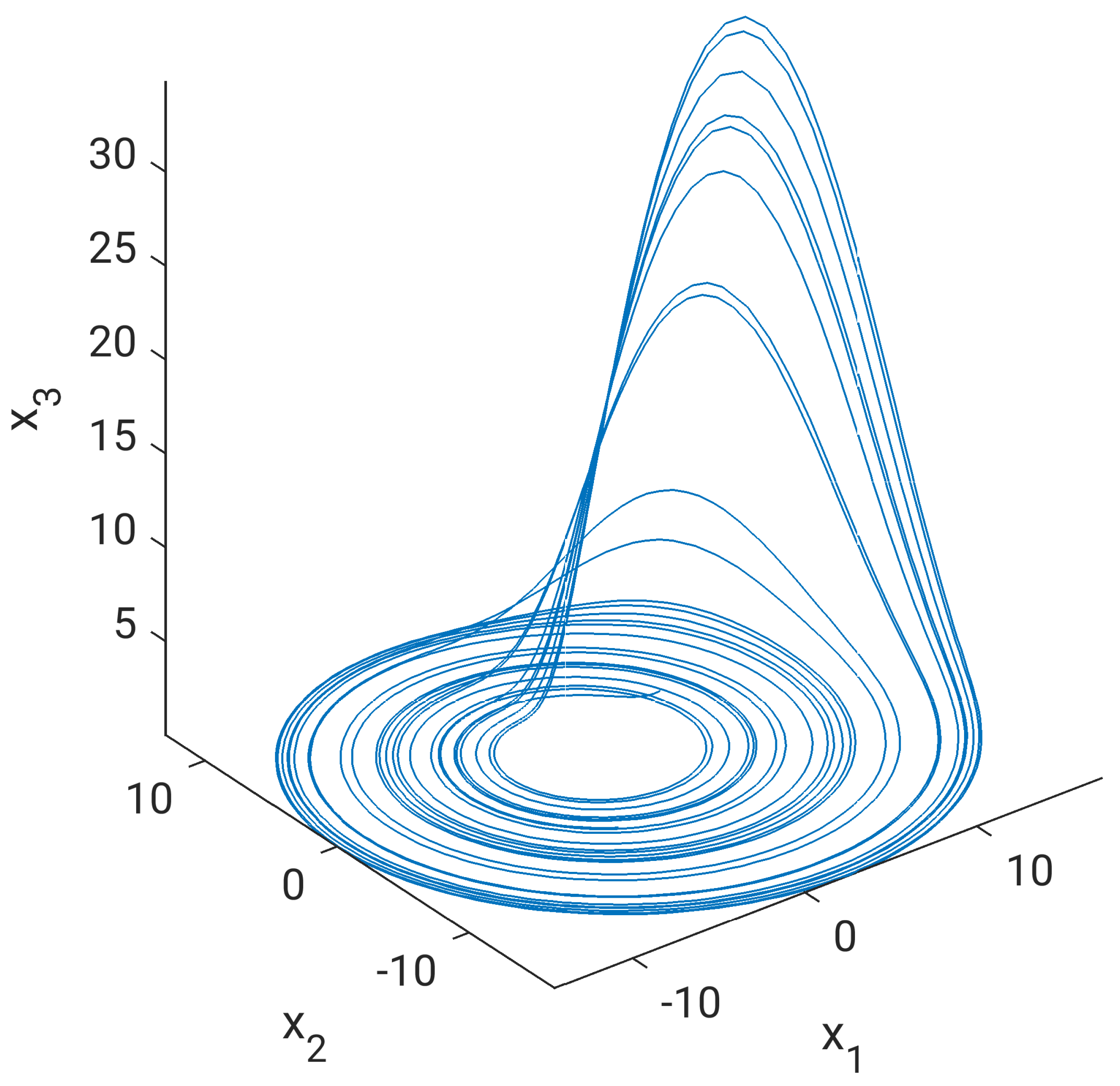
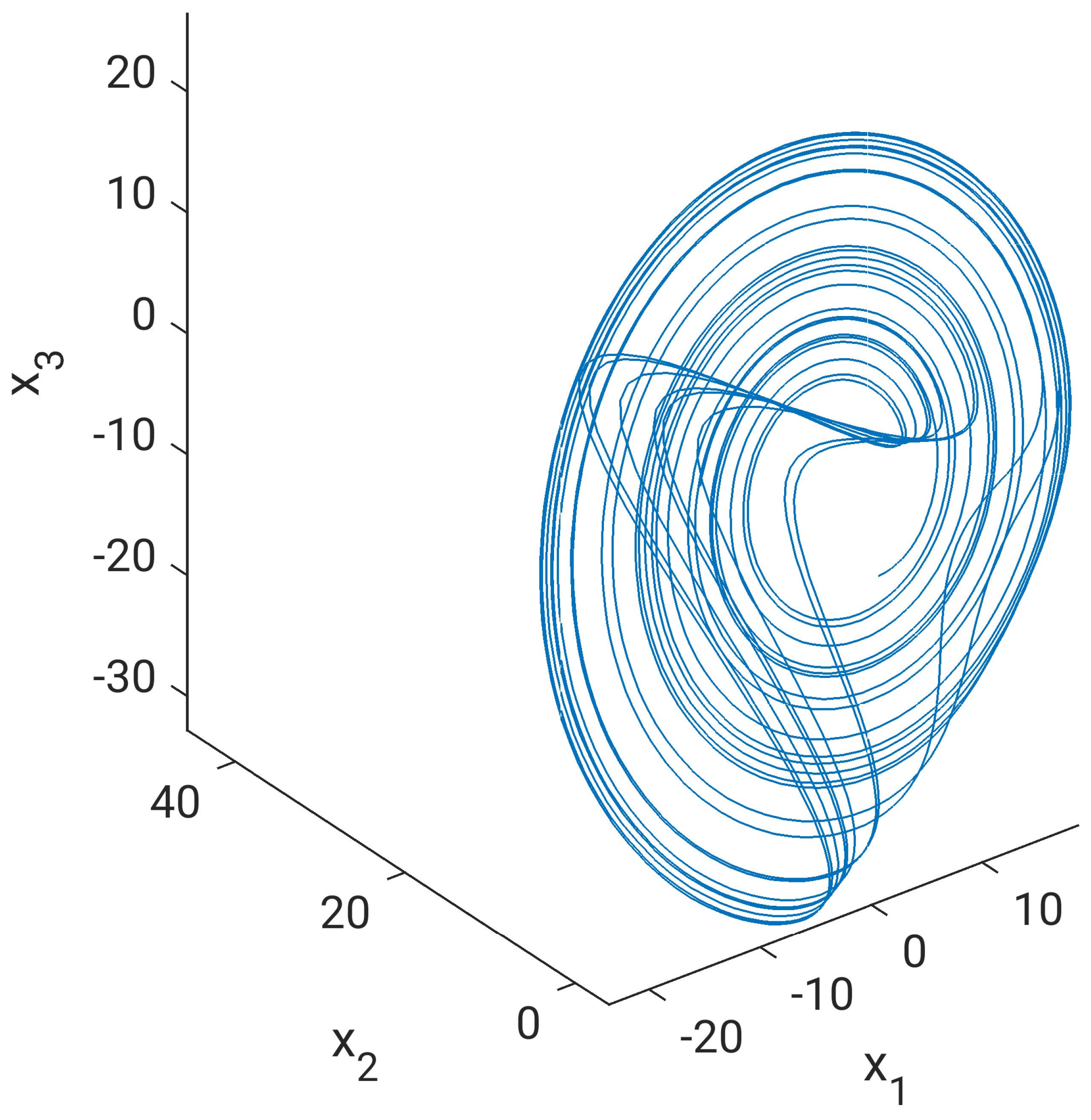
Our results are illustrated in Figure 1, Figure 2 and Figure 3 below. Alongside the original trajectory, $x\left(t_i\right)$, we also plot the reconstructed trajectory obtained via the DyCA, as well as a reconstruction of the signal by means of a thin SVD of Q.

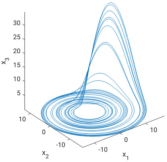
Figure 1. DyCA applied to a trajectory of the Rössler system: original signal.

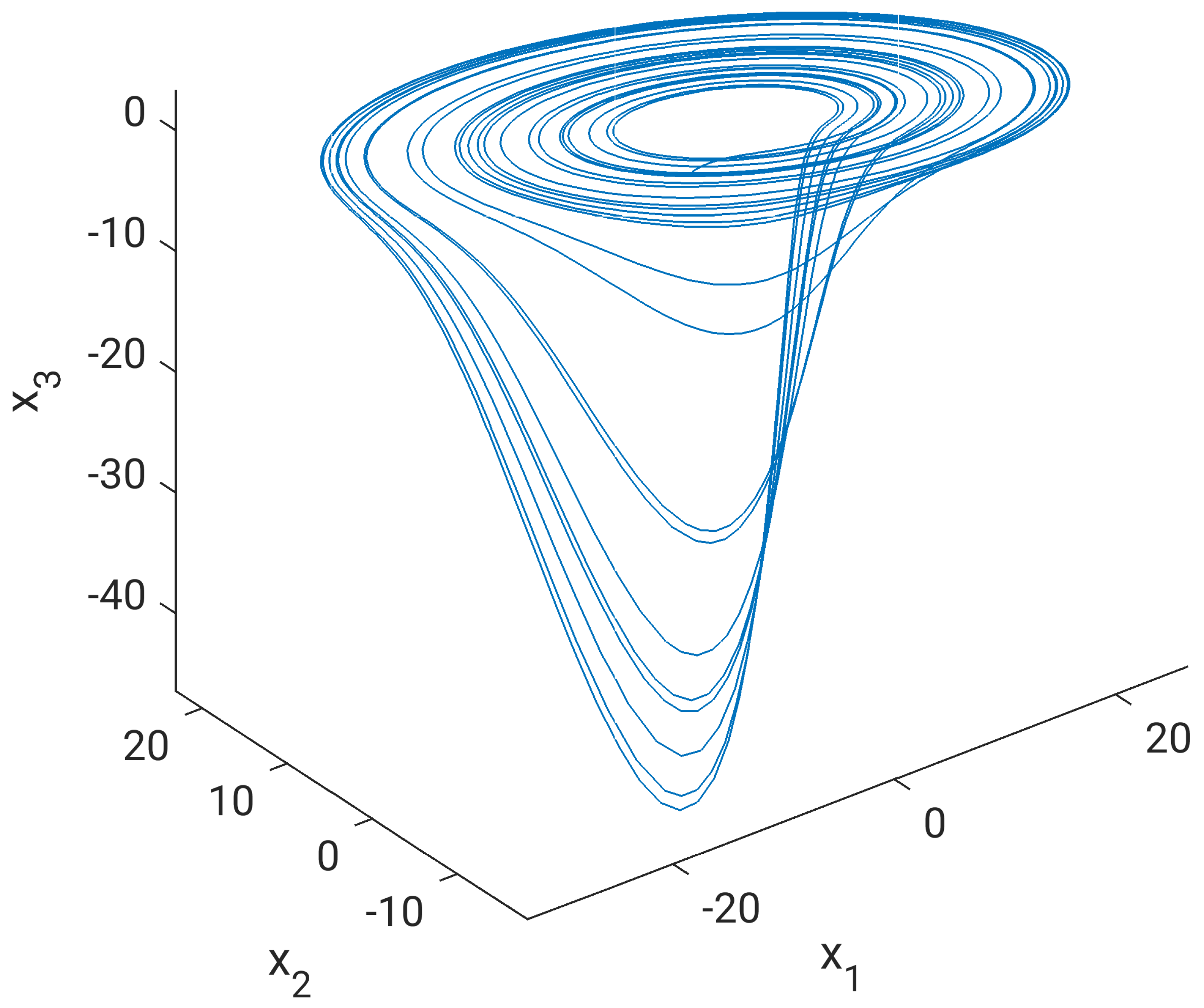
Figure 2. DyCA applied to a trajectory of the Rössler system: projection via DyCA.

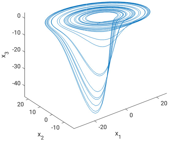
Figure 3. DyCA applied to a trajectory of the Rössler system: SVD-based projection.

6.2. Lorenz System

We also apply DyCA to the Lorenz system

$$\begin{array}{cc}\hfill {\dot{x}}_1\left(t\right)& =a(x_2\left(t\right)-x_1\left(t\right)),\hfill \\ \hfill {\dot{x}}_2\left(t\right)& =x_1\left(t\right)(b-x_3\left(t\right)-x_2\left(t\right)),\hfill \\ \hfill {\dot{x}}_3\left(t\right)& =x_1\left(t\right)x_2\left(t\right)-c{x}_3\left(t\right),\hfill \end{array}$$

(55)

where $a=10,b=28$, and $c=8/3$. Accordingly, by defining $A=\left[\begin{array}{ccccc}-a& & a& & 0\end{array}\right]$ and

$$\begin{array}{cc}\hfill f:{\mathbb{R}}^3& \to {\mathbb{R}}^2,\hfill \\ \hfill \left[\begin{array}{c}{x}_1\\ x_2\\ x_3\end{array}\right]& \mapsto f(x_1,x_2,x_3):=\left[\begin{array}{c}{x}_1(b-x_3-x_2)\\ x_1{x}_2-c{x}_3\end{array}\right],\hfill \end{array}$$

(56)

we rewrite Equation (55) as follows:

$$\begin{array}{cc}\hfill [I_1,0]\dot{x}\left(t\right)& =Ax\left(t\right)\hfill \\ \hfill [0,I_2]\dot{x}\left(t\right)& =f\left(x\right(t\left)\right).\hfill \end{array}$$

(57)

Thus, (55) is written in the form of Equation (2), where $n=3$ and $m=1$. Hence, we may apply Algorithm 1 to solve Problem 1, where the low-dimensional dynamics of the signal satisfies the ODE Equation (55).

We also indicate this via another numerical experiment. Analogously to the Rössler system discussed above, we create a mixing matrix $W\in {\mathbb{R}}^{N\times n}$, where $N=30$, and we generate the signal Q and its time derivative by integrating Equation (55) using the MATLAB function ode45. Similar to Figure 1, Figure 2 and Figure 3, we present the results obtained for the Lorenz system in Figure 4, Figure 5 and Figure 6 below.

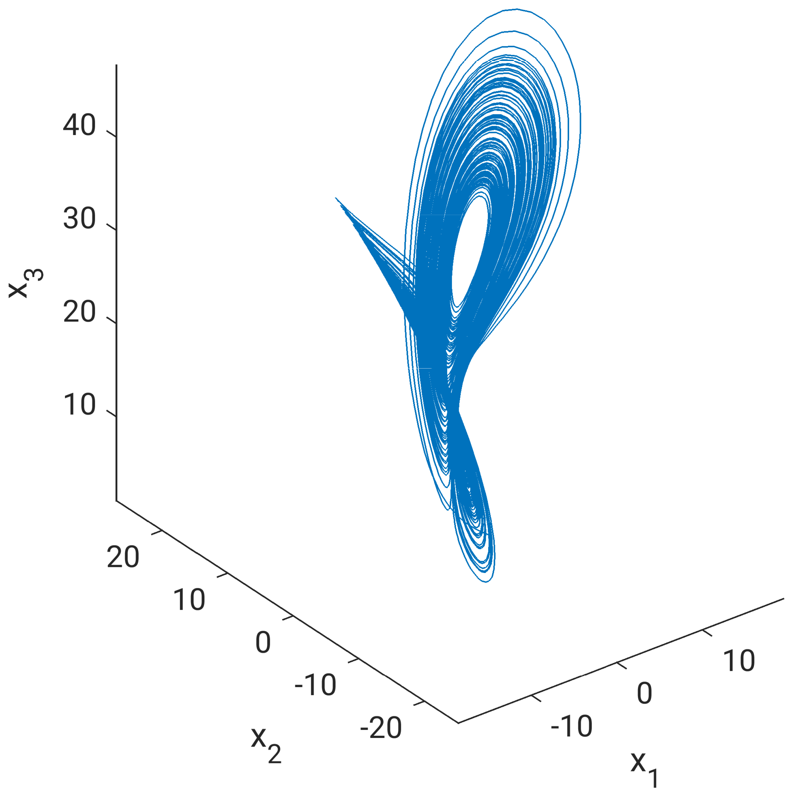
Figure 4. DyCA applied to a trajectory of the Lorenz system: original signal.

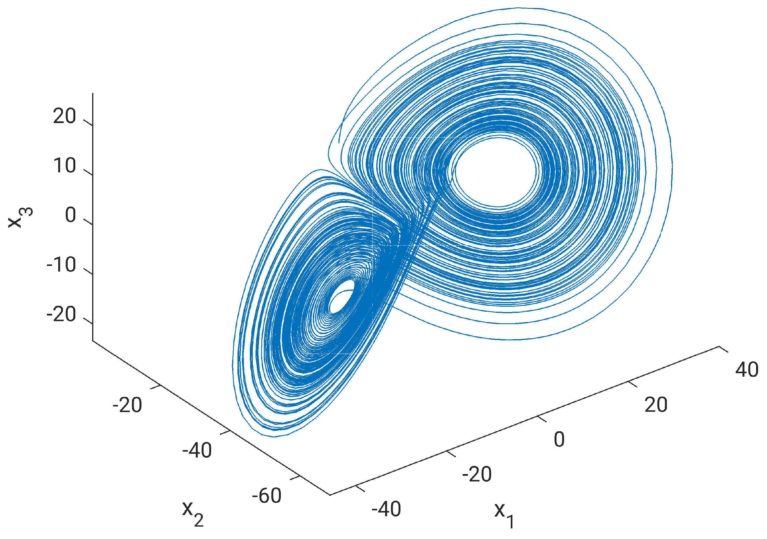
Figure 5. DyCA applied to a trajectory of the Lorenz system: projection via DyCA.

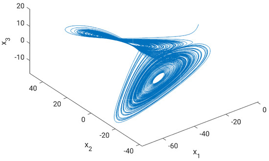
Figure 6. DyCA applied to a trajectory of the Lorenz system: SVD-based projection.

7. Outlook and Discussion

In this paper, we have discussed a reformulation of the so-called DyCA problem, putting the original cost function approach into perspective with respect to an inverse problem formulation. It is certainly out of scope for this paper to discuss more advanced techniques from the vast area of numerics for inverse problems. In particular, to acknowledge the fact that one is ultimately interested in the inverse of the mixing matrix in the case of noise, a possibly ill-posed problem. For results in this direction, we refer the reader to forthcoming papers including real-world data, e.g., analyzing EEG data. We, however, have shown so far that for the two examples (Lorenz and Rössler) where data were generated artificially, our results are promising; in particular, for data corrupted only by a reasonable amount of noise, the algorithm works well.

Clearly, any questions related to scalability, usability, or complexity in the above context can be easily addressed via the vast body of existing literature on singular-value decomposition-based algorithms from the last 30 years, either from the numerical linear algebra community or from the pertinent signal processing literature.

References

- Korn, K.; Seifert, B.; Uhl, C. Dynamical Component Analysis (DYCA) and Its Application on Epileptic EEG. In Proceedings of the ICASSP 2019—2019 IEEE International Conference on Acoustics, Speech and Signal Processing (ICASSP), Brighton, UK, 12–17 May 2019; pp. 1100–1104. [Google Scholar] [CrossRef]
- Uhl, C.; Kern, M.; Warmuth, M.; Seifert, B. Subspace Detection and Blind Source Separation of Multivariate Signals by Dynamical Component Analysis (DyCA). IEEE Open J. Signal Process. 2020, 1, 230–241. [Google Scholar] [CrossRef]
- Romberger, P.; Warmuth, M.; Uhl, C.; Hüper, K. Dynamical Component Analysis: Matrix Case and Differential Geometric Point of View. In Proceedings of the CONTROLO 2022, Caparica, Portugal, 6–8 July 2022; Brito Palma, L., Neves-Silva, R., Gomes, L., Eds.; Springer: Cham, Switzerland, 2022; pp. 385–394. [Google Scholar] [CrossRef]
- Schlarb, M.; Hüper, K. Optimization on Stiefel Manifolds. In Proceedings of the CONTROLO 2022, Caparica, Portugal, 6–8 July 2022; Brito Palma, L., Neves-Silva, R., Gomes, L., Eds.; Springer: Cham, Switzerland, 2022; pp. 363–374. [Google Scholar] [CrossRef]
- Seifert, B.; Korn, K.; Hartmann, S.; Uhl, C. Dynamical Component Analysis (DYCA): Dimensionality Reduction for High-Dimensional Deterministic Time-Series. In Proceedings of the 2018 IEEE 28th International Workshop on Machine Learning for Signal Processing (MLSP), Aalborg, Denmark, 17–20 September 2018; pp. 1–6. [Google Scholar] [CrossRef]
- Paglia, C.; Stiehl, A.; Uhl, C. Identification of Low-Dimensional Nonlinear Dynamics from High-Dimensional Simulated and Real-World Data. In Proceedings of the CONTROLO 2022, Caparica, Portugal, 6–8 July 2022; Brito Palma, L., Neves-Silva, R., Gomes, L., Eds.; Springer: Cham, Switzerland, 2022; pp. 205–213. [Google Scholar] [CrossRef]
- Rössler, O. An equation for continuous chaos. Phys. Lett. A 1976, 57, 397–398. [Google Scholar] [CrossRef]
Disclaimer/Publisher’s Note: The statements, opinions and data contained in all publications are solely those of the individual author(s) and contributor(s) and not of MDPI and/or the editor(s). MDPI and/or the editor(s) disclaim responsibility for any injury to people or property resulting from any ideas, methods, instructions or products referred to in the content. |
© 2024 by the authors. Licensee MDPI, Basel, Switzerland. This article is an open access article distributed under the terms and conditions of the Creative Commons Attribution (CC BY) license (https://creativecommons.org/licenses/by/4.0/).