Abstract
This paper presents the use of continuous wavelet transform (CWT) to capture the frequency contents, spectra of dominant frequencies and associated time durations of real earthquakes for generating artificial excitations to perform endurance time analysis (ETA) of structures. Applying CWT to three sets of forty earthquakes, the 90 percentile frequencies that span the ranges 0.08–18.41 Hz, 0.61–12.73 Hz, and 0.56–15.53 Hz; with associated time durations of 20, 15 and 16 s, respectively, for these earthquake sets are extracted. Artificial excitations that contain these ground motion characteristics are generated, progressively scaled up and applied to the target structure until failure. The scaling used is a block-shaped envelope that increases in size by a factor of 3/2 over time. Nonlinear seismic analyses of a steel frame and a concrete bridge bent using these artificial excitations have shown that the method not only successfully predicts the base shear–roof displacement responses of these structures, it also correctly identifies behavior such as weak story, concrete spalling, and core cracking. When compared with the increment dynamic analysis and time history analysis using multiple earthquakes, the proposed method is capable of producing comparable results with a significant reduction in computational time and a much smaller output file size.
1. Introduction
Earthquake engineering has undergone many important advances over the last century. What started as a push to save lives in anticipation of future seismic events has developed into an effort not just to ensure life safety, but to limit structural damage and minimize repair time at levels considered acceptable by both designers and owners. Earthquake engineers utilize performance-based seismic design (PBSD) strategies to design structures with a predictable and predefined seismic performance under a given severity of the hazard. These strategies have been developed based on past experiences of structural responses to earthquake excitations, as well as preconceptions regarding the impact that real seismic events have on particular types of structures [1].
Based on the level of significance of the structure and the degree of past seismicity at a given site, various methods of seismic analysis and design can be utilized. On the analysis side, the equivalent static, response spectrum and time history analysis (THA) methods are perhaps the most well-known as they have been codified in ASCE 7-22 [2] and IBC 2021 [3]. Other analysis techniques that can be used in performance-based seismic analysis and design are nonlinear static (also referred to as “pushover”) analysis [4] and nonlinear dynamic analysis [2].
There are two types of nonlinear dynamic analyses, referred to as wide-range and narrow-range analyses. Wide-range analyses are reasonable for use in making probabilistic evaluations of structural responses over a wide range of tolerable probability extents, while narrow-range analyses are suitable for use in making probabilistic investigations over a narrower range of tolerable probability values. Multiple-stripe analysis (MSA) [5] and incremental dynamic analysis (IDA) [6] are two examples of wide-range analyses, while single-stripe analysis (SSA), and double-stripe analysis (DSA) [7] are examples of narrow-range analyses.
Multiple-stripe analysis can be used to evaluate structures over a range of earthquake intensities and performance targets that range from Immediate Occupancy (IO) to Collapse Prevention (CP) levels. Specifically, single-stripe and double-stripe analysis can be used to evaluate a local probabilistic engineering demand utilizing fewer numbers of nonlinear analyses (around 20 to 40).
In an incremental dynamic analysis (IDA), an excitation function is scaled progressively to various intensity measure (IM) levels. The largest engineering demand parameter (EDP) is calculated for every scale level [6]. Although IDA can give a decent estimation of structural response at different IM levels and can be used to compute the global instability limit state, the large number of nonlinear analyses that are required makes IDA undesirable for application on a routine basis. Analyzing structures using IDA is very computationally intensive and time-consuming.
The endurance time analysis (ETA) method [8] was developed to reduce computational effort without sacrificing accuracy. In ETA, heuristic methodologies are utilized to develop endurance time excitation functions (ETEFs), which can then be used to generate an intensifying seismic event. ETA can be used to assess structural responses at different excitation levels from linear elastic to nonlinear stages, as well as up to the global collapse of the structure, all in one single analysis [9].
The dynamic response of a system is highly dependent on the input ground motion characteristics, especially when the system response is in the nonlinear range. There are two commonly used domains in characterizing ground motions: time and frequency. In the time domain, ground motion characteristics such as peak ground acceleration (PGA), the time at which PGA occurs, and the overall duration of the ground excitation are used. However, the frequency content of the earthquake is not known. On the other hand, characterizing ground motions in the frequency domain using Fourier Transform (FT) allows only the frequency content to be extracted. The temporal aspect of the dominant frequency and the spectrum of frequencies that are considered the most important in affecting system response are lost.
The present research uses Morse wavelet to perform continuous wavelet transform (CWT) of real earthquakes to identify both time and frequency characteristics of these earthquakes with the aim of generating better artificially generated ground motions. Using CWT, important earthquake attributes such as frequency content, the spectrum of dominant frequencies and the associated time duration within which these frequencies occur are extracted. This information is then used to generate artificial ground motions referred to as endurance time excitation functions (ETEFs) to perform ETA. The use of ETA in conjunction with the ETEFs proposed in the present work allows for a noticeable reduction in computational time and effort without sacrificing accuracy, even for structures that experience high nonlinearity in both geometry and material.
The primary objectives of this study are to:
- -
- Investigate various real earthquakes via continuous wavelet transform in the time-frequency domain.
- -
- Extract important ground motion characteristics from these earthquakes for use in generating new endurance time excitation functions (ETEFs).
- -
- Generate ETEFs with ground motion characteristics that match the geometric mean response spectrum of these real earthquakes.
- -
- Perform endurance time analyses on steel and reinforced concrete structures using these ETEFs and compare the results with those obtained from an incremental dynamic analysis (IDA), which is considered to be the most sophisticated method of analysis; or the time history analysis (THA) using multiple earthquakes.
In the next section, the essence of ETA is described. This is followed by a brief discussion of CWT used in the present analysis. Detailed procedures for generating ETEFs based on real earthquakes with different magnitudes and soil site conditions are then discussed. Examples are given to demonstrate the validity of the proposed method.
2. Endurance Time Analysis (ETA) Method
The concept behind the endurance time analysis (ETA) method can best be described by considering the time it takes for several structures with different seismic resistance characteristics to experience distress when subject to the same artificial ground excitation with a slowly increasing magnitude [8]. The structure that is the first to experience distress and collapse is considered the least desirable and the structure that perseveres (endures) the longest is considered the most desirable. It should be noted that this conclusion is based solely on how long a structure can withstand the intensifying excitation (i.e., its endurance time), with no reference to the structure’s stiffness and strength or other system parameters. This method of analysis provides an immediate and important measure to investigate structural performance and forms the basic concept behind the ETA method. In ETA, structures are graded by the time they can withstand a gradually intensifying ground excitation. A longer endurance time means better performance. The performance of a structure is evaluated by the time (which is related to ground motion intensity) when a predefined damage index (e.g., drift, plastic energy, etc.) is reached or surpassed.
One important element of utilizing ETA is the generation of artificial excitation functions. In the first generation of artificial excitation functions, a random vibration modified through filtering in the frequency domain was made to be compatible with the geometric mean response spectrum of earthquake records. This stationary excitation function was then modified by multiplying it by a linear profile to intensify the amplitude of the excitation as a function of time [8]. The second generation of ETEF was developed based on matching a predefined response spectrum that grows with time, and these have been shown to produce noteworthy results [10]. The third generation of ETEFs was generated to address nonlinear response spectra analysis issues and optimize the implementation of the method, while the fourth generation of ETEFs used an exponentially increasing profile of excitation functions and was developed to include signal duration and the proper intensity [11].
The ETA method has been successfully utilized for the linear analysis of structures [9], nonlinear seismic evaluation of single-degree-of-freedom (SDOF) systems [12] and seismic analysis of multi-degrees-of-freedom (MDOF) systems [13,14,15]. Furthermore, Valamanesh and Estekanchi [16] studied the seismic response of steel frames using the ETA procedure, while Alembagheri and Estekanchi [17] employed the ETA method to study the vibration response of steel water storage tanks. Tavazo et al. [18] employed ETA in conjunction with time history analysis to analyze various shell structures. The results of these analyses have shown good agreement with those obtained using time history analysis. Zeinoddini et al. [19] used the concept of ETA to develop the endurance wave analysis (EWA) technique with the goal of determining the response of offshore structures under extreme waves. Valamanesh et al. [20] applied ETA to investigate the seismic response of gravity dams, and Hariri-Ardebili et al. [21] explored the use of ETA in the nonlinear analysis of a curve dam and concluded that ETA was able to track the crack patterns developed in the dam. Shirkhani et al. [22] utilized the ETA method to investigate the performance of steel structures using rotational friction dampers (RFD) to calculate the optimum slip force of the RFD. Basim and Estekanchi [23] used ETA to assess the application of the method in the performance-based optimum design of steel frames. Foyouzat and Estekanchi [24] investigated the application of the ETA method to generate rigid-perfectly plastic spectra to improve seismic response assessment.
By the late 2010s and early 2020s, the ETA method developed and evolved into a practical method for analyzing and designing a variety of structures under seismic excitations. For instance, Mashayekhi et al. [25] developed hysteretic energy-compatible endurance time excitations for determining local and global damage in concrete frames. Li et al. [26] proposed an improved ETA method and applied it to four reinforced concrete frames with 4, 8, 12, and 16 stories to verify the validity of the method. Hasani et al. [27], Bai et al. [28] and Sarcheshmehpour et al. [29] applied the ETA method to include soil-structure interaction effects; while Shirkhani et al. [30,31] extended their previous work [22] and further incorporated the use of supplementary dampers in their analyses of frame systems. The use of ETA for seismic analysis of bridges has been reported by Guo et al. [32], Ghaffari et al. [33], He et al. [34], and Pang et al. [35]. Mirfarhadi and Estekanchi [36] proposed a value-based seismic design procedure for structures based on performance assessment by the ETA method. Mohsenian et al. [37] performed a multi-level response modification factor estimation for steel moment frames, and Xu et al. [38] developed a modified ETA algorithm that accounts for the duration effect of strong ground motions to estimate the earthquake resistance and seismic performance of a concrete gravity dam.
The straightforward and sensible nature of the method as well as its applicability to a wide range of structures, including the most complex ones, have made it quite attractive for use in assessing structural response to seismic excitations [39]. ETA is particularly effective in assessing structural performance since it is characteristically similar to IDA but requires much less computational time and effort.
3. Wavelet Transform and Wavelet Analysis
Wavelet analysis was initially developed and used by mathematicians and seismologists for processing seismic signals [40,41]. Wavelet transform [42] is a type of mathematical transform that involves two parameters. For a time signal f(t), the two parameters are scale (s) and position (p). Depending on the type of wavelet that is being used, the s parameter can be correlated with frequency and the p parameter can be related to time. An important aspect of applying wavelet transform is choosing an appropriate wavelet function ψ(t) from a number of wavelets called mother wavelets [43]. One desirable attribute of wavelet transform is that, in addition to extracting the frequency content of the signal, it provides information on the temporal nature of these frequencies.
3.1. Wavelet Coefficients
To conduct the transform, the selected mother wavelet is first scaled by the s parameter and shifted by the p parameter to form the so-called daughter wavelets ψs,p(t) using the equation
Scaling a wavelet means extending or compressing it. The smaller the scale s, the more compressed the wavelet is, and vice versa. In wavelet analysis, the scale is related to the frequency of the signal. Shifting a wavelet essentially implies delaying its onset. Delaying a mother wavelet by p is represented by .
To perform the wavelet transform of a given time signal f(t), the time signal is multiplied by the daughter wavelet and integrated over the time domain from −∞ to ∞.
The above equation is called the integral or continuous wavelet transform. By carrying out the integration, often numerically, using different values of s and p, an array of wavelet coefficients C can be obtained. Multiplying each C by a properly scaled and shifted wavelet produces a series of constituent wavelets of the original signal.
3.2. Wavelet Map
Wavelet transform produces wavelet coefficients C that are functions of scale and position. In wavelet analysis, a wavelet with designated s and p values is matched against a segment of an actual signal, and the wavelet coefficient C is calculated for that segment. A high C value means this wavelet closely resembles that segment of the signal. The process is repeated for another segment of the signal until the entire signal is covered. Once all the wavelet coefficients are calculated, they can be plotted on a wavelet map. On a wavelet map, the x-axis represents the position (or time) of the signal, the y-axis represents the scale (related to frequency) of the signal, and the different shades on the x-y plot represent the magnitude of the wavelet coefficient C. A light or bright color shade means there is a high correlation between the wavelet and the original signal.
3.3. Morse Wavelets
In the present work, Morse wavelets were used to perform continuous wavelet transform analysis to identify both time and frequency characteristics of real ground motions. Morse wavelets are utilized to analyze modulated signals. Modulated signals are signals with time-varying amplitude and frequencies [44]. The theory of Morse wavelets and their applications are described in a series of literature by Lilly and Olhede [45,46,47].
Morse wavelets, represented as , are defined in the frequency domain for order ≥ 0 and family > 0 as:
where is the angular frequency, and is a real-valued normalizing constant given by:
in which ≈ 2.71828 is Euler’s number. The order controls the low-frequency behavior, and the family controls the high-frequency decay. Differentiating with respect to , Morse wavelets attain their maximum value (the peak frequency) at the frequency:
By changing the values of and , a wide range of time-domain forms of the Morse wavelets can be obtained. As and increase, the functions become more oscillatory and as these parameters decrease, the functions become more localized, appearing as isolated events in the time domain. For a given , increasing gives function modulus curves that are less strongly concentrated about its center and for a given , increasing packs more oscillations into the same envelope [48].
Morse wavelets in conjunction with continuous wavelet transform were used in the present work to extract earthquake characteristics which were then used to create artificial excitation functions that matched with the geometric mean response spectra of both normal and parallel components of three sets of forty real ground motions contained in a PEER report [49]. These artificial excitation functions were then scaled by intensifying blocks for use in endurance time analysis of elastic and inelastic structures.
4. Generation of Artificial Ground Motions and ETEFs
Nonlinear dynamic assessment of structures requires the use of a large number of earthquake data if the goal is to correlate structural performance with various damage parameters, as is the case for performance-based seismic design. Although earthquakes occur in a number of earthquake-prone regions around the world (https://www.emsc-csem.org/#2w, accessed on 13 June 2023), the number of recorded ground motion data for a given site could be limited. As a result, to acquire the needed number of ground motions for a given site condition, scaling and spectral matching are often used to modify available ground motion records so they are more representative of the specific site conditions. Instead of using scaling and spectral matching of real earthquakes, one can create artificial excitations capable of mimicking both the physical conditions and qualities of real earthquakes. In the present study, three artificial excitations were generated using three sets of forty real ground motion data. The process to generate these three artificial excitations is described in the following sections.
4.1. Ground Motion Data
The three sets of forty ground motions used are labeled Set#1a, Set#1b and Set#2 (Appendix A). They were obtained from the PEER NGA Project ground motion library [50] and had been rotated from their as-recorded orientations to the fault normal (FN) and fault parallel (FP) directions by Baker et al. [49]. According to Baker et al. [49], Set#1a was selected so their horizontal response spectra from 0 to 5 s (the period range of interest for systems being considered in the study) would match the median and log standard deviation of a moment magnitude 7 strike-slip earthquake 10 km from the fault. The site’s average shear wave velocity in the top 30 m (Vs30) was taken as 250 m/s (i.e., soil site). Set#1b was selected so their horizontal response spectra from 0 to 5 s would match the median and log standard deviation of a moment magnitude 6 strike-slip earthquake at 25 km from the fault. Like Set#1a, the site’s Vs30 was taken as 250 m/s. Set#2 was selected so their response spectra from 0 to 5 s would match the median and log standard deviation of a moment magnitude 7 strike-slip earthquake at 10 km from the fault. However, the site’s Vs30 was taken as 760 m/s. A larger Vs30 was used for Set#2 so these ground motions would mimic those that occur at a rock site.
4.2. Wavelet Maps
Applying continuous wavelet transform (CWT) with Morse wavelets to the aforementioned three sets of 40 earthquakes (i.e., a total of 120 earthquakes), the wavelet maps for these earthquakes, including the wavelet coefficients C in two dimensions and their absolute values, were obtained. As mentioned earlier, C represents how closely the wavelet is correlated with the actual signal. The higher the value of C, the more closely the wavelet resembles the signal. From an energy standpoint, if both the signal energy and the wavelet energy are normalized to one, C may be interpreted as a correlation coefficient. Note, that decomposed signals can be combined to obtain signal components at various scales. By examining the wavelet maps, one can observe that the original accelerogram has a dominant component signal shown as the lightest color. It is interesting to note that light-colored regions in the wavelet map correspond to locations of higher accelerations in the recorded ground motion.
From a given wavelet map, the frequency range (the lowest and highest frequencies of the ground motion), the dominant frequency (the frequency with the highest C value), the window of frequencies (the frequencies with a C value within 10% of the dominant frequency) and the corresponding time span (the length of time within which these frequencies occur) can be obtained for each component (FN, FP) or each of the ground motion records. To illustrate the procedure, the windows of frequencies and time spans obtained for two sample ground motion records, RSN 161 and RSN 266 (see Appendix A for more details about these two earthquakes), are shown in Figure 1a,b, respectively. Note, that the scale used for the vertical axis of the wavelet maps is logarithmic.
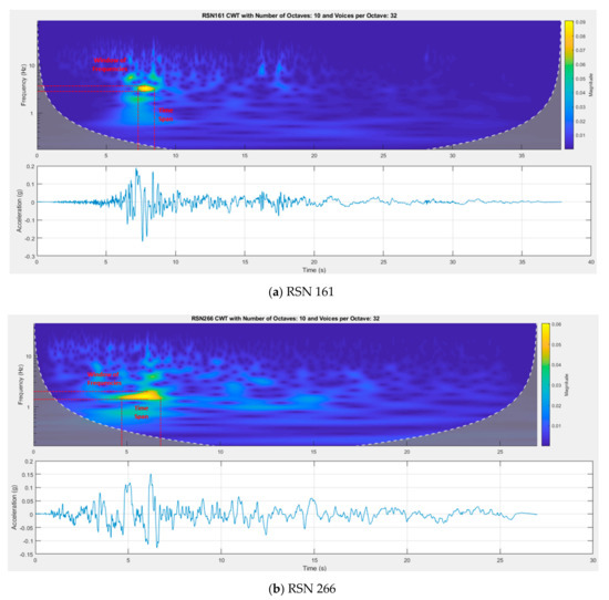
Figure 1.
Window of frequencies and time spans.
Repeating the above procedure for all 120 ground motion records, the dominant frequency and the frequency range for each ground motion component for Set#1a, Set#1b, and Set#2 were obtained and are shown in Figure 2. The frequency range is a signature of the earthquake. It is an important parameter for use in generating artificial excitations as frequencies outside of this range are filtered out and only frequencies within the range are retained.
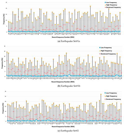
Figure 2.
Dominant and range of frequencies.
The time spans or time durations within which the dominant and window of frequencies occur for these three sets of earthquakes are shown in Figure 3. These time durations are important in establishing an envelope for artificial excitation functions. The artificial excitation functions are to be generated so they will contain a large percentage (>90%) of the extracted frequencies and time durations.
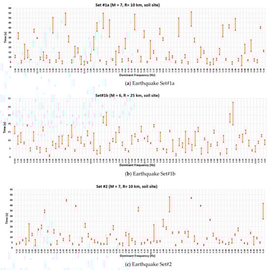
Figure 3.
Time durations.
From the data given in Figure 2 and Figure 3, statistical analyses were performed using @RISK software [51] to determine the probability distribution function (PDF) that best fits these data. Based on the Akaike Information Criterion (AIC) [52], the PDF was determined to be a lognormal distribution. For each earthquake set, the low and high frequencies as well as the time duration obtained from this lognormal PDF that encompasses at least 90% of the frequency data and the 90 percentile of the time durations were obtained and presented in Table 1. These spectra of frequencies will be used as the basis to filter out frequencies that are randomly generated. Randomly generated frequencies that fall outside of this range are to be discarded.

Table 1.
Summary of frequencies and time durations for the three earthquake sets.
4.3. Generation of Artificial Excitations
The software SeismoArtif [53] was used to generate artificial excitations. The response spectrum of the artificial excitation needs to match against a target spectrum, which in the present analysis was taken as the geometric mean spectrum of the real ground motions obtained for each respective earthquake set. To ensure that the frequency contents of these artificial excitations fall within the frequency range given in Table 1, the sixth-order Type 1 Chebyshev filter function [54] was used. This filter function is capable of providing a sharp roll-off and is deemed appropriate for the present application as it can be used to filter out excessive frequencies and keep all necessary frequencies in the generated artificial excitations. A downside of the Chebyshev filter is the presence of maxima and minima in gain (called gain ripples) in the passband. However, the ripple effect can be minimized by using a small value of gain ripple. In the present work, a 1 dB gain ripple was utilized to minimize the ripple effect. By using this filter, frequencies outside of the passband were filtered out and the remaining frequencies that correspond to the frequency range obtained from the original ground motion records were then used to construct the artificial excitations.
In addition, the choice of an appropriate time duration for each of the artificial excitations was also given due consideration. For a linearly elastic system, the value used for the time duration can be arbitrary as it does not have any significant effect on the results. This is because a scale factor can be used to scale the accelerogram to reach a spectral acceleration Sa (or spectral displacement Sd) value that matches the required target level at any desired time. However, for systems that exhibit nonlinearity, the selection of the proper time duration is important. If the time duration is set too low, the structure may not have sufficient time to go through a reasonable number of nonlinear cycles and experience all pertinent excitation frequencies. On the other hand, if the time duration is set too high, the number of cycles will become unrealistically high. In the present work, the time durations for artificial excitation Set#1a, Set#1b and Set#2 were set at 20 s, 15 s and 16 s, respectively, as given in Table 1. The 5% damping artificial excitations generated in this manner that match the geometric mean response spectra of Earthquake Set#1a, Set#1b and Set#2 are shown in Figure 4. A comparison of response spectra is given in Figure 5.
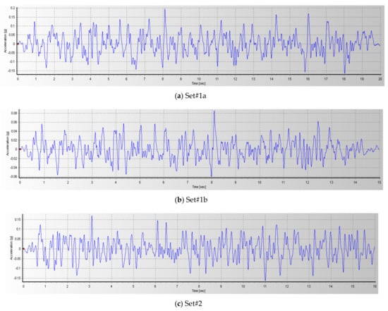
Figure 4.
Artificial excitations (5% damping).
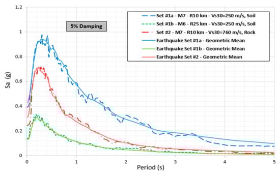
Figure 5.
Comparison of response spectra (5% damping).
4.4. Generation of Intensifying ETEFs
To generate the endurance time excitation function (ETEFs), the artificially generated excitation for each earthquake set was intensified using the block envelope shown in Figure 6a. It is in the form of a series of expanding blocks obtained by scaling the artificially generated excitation by a scale factor of 2/3, 1 and 1.5, respectively, (i.e., each successive envelope is obtained by increasing the size of the previous envelope by a factor of 3/2) to represent the increase in excitation intensity. It should be noted that the scale factor 2/3 corresponds to that used in ASCE 7-22 [2] to obtain Design Earthquake from the Maximum Considered Earthquake. As an example, the resulting ETEF generated for artificial excitation Set#1a for 5% damping is shown in Figure 6b. Note, the excitation pattern is repeated in each block with the magnitude increasing from one block to the next.
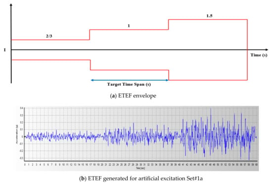
Figure 6.
Block-shaped intensifying envelope.
5. Application of ETA to Steel and Concrete Structures
Structures are often designed to respond inelastically under strong earthquakes. This means they need to be analyzed and designed as nonlinear systems. Structures that are designed, detailed, and constructed to withstand a certain amount of inelastic deformations should survive a strong earthquake without experiencing excessive deformations or collapse. In this section, the analysis results of two structures—a FEMA 440 benchmark steel frame structure and a PEER concrete column—are presented. Each structure was subjected to an artificially generated ETEF described in the preceding section. The analysis results are then compared to those obtained using the incremental dynamic analysis (IDA) method.
The main goal of studying these systems is to show how the artificially generated ETEF can be used to predict the performance of structures and to demonstrate how well the analysis results are when compared with those obtained using more precise (but computationally intensive) IDA or THA method using multiple ground motion records.
For both systems, the system of equations that needs to be solved is
where M is the mass matrix, C is the damping matrix, R(t) is the vector of the system’s restoring force. and are the acceleration and velocity vectors, respectively, and g(t) is the ground acceleration, which in conducting endurance time analysis (ETA) is the endurance time excitation function (ETEF).
5.1. FEMA 440 Benchmark Steel Frame Structure
The steel moment-resistant frame was designed as part of the FEMA-funded SAC joint-venture project [55]. The original design was based on the 1994 Uniform Building Code [56] including the use of special moment-resisting connections. Special moment connections are connections that are capable of accommodating a story drift angle of at least 0.04 radian. In addition, at a story drift angle of 0.04 radian, the measured flexural resistance of the connection at the column face shall equal at least 0.08 Mp of the connected beam, where Mp is the plastic moment capacity of the beam [57]. The first story of the building was designed to act as a weak story in that the columns in this story were expected to develop a story failure mechanism under a ground motion that would cause the peak roof displacement of the frame to reach 4% of the building’s height when any dynamic analysis, such as the time history analysis or the incremental dynamic analysis, was used.
The four-bay frame, which consists of wide-flange (W) sections shown in Figure 7, has a floor-to-floor height of 13 ft (4 m) and a bay width of 30 ft (9.15 m) and is subject to the loading given in Table 2. Note, that the beams of the rightmost bay are pinned at both ends, but the beams of the other bays have moment-resisting connections. The materials used for the beams and columns have yield stresses of 49.2 ksi (340 MPa) and 57.6 ksi (397 MPa), respectively.
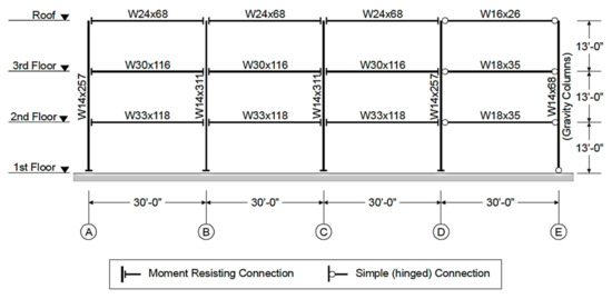
Figure 7.
Three-story steel frame (1′ = 0.305 m).
Table 2.
Loading used for three-story steel frame (1 psf = 47.9 N/m2).
The frame was modeled in SeismoStruct [58] using the inelastic displacement-based plastic hinge frame element (infrmDBPH). This is a twelve degrees-of-freedom 3D displacement-based plastic hinge element that allows concentrated plastic hinges to form at its ends (Figure 8). The formulation is based on the model developed by Giberson [59], which includes an elastic element with four nonlinear rotational springs located at the ends of the element in two different local axes. Nonlinear deformations are confined to these rotational springs. Each beam and column was modeled using nine infrmDBPH elements. The material model used was the Menegotto–Pinto steel model [60], which is a uniaxial material model initially presented by Yassin [61] using the stress-strain relationship proposed by Menegotto and Pinto [60] in conjunction with the isotropic steel hardening model of Filippou et al. [62]. Using this material model, the hysteresis loops generated for the columns and beams are shown in Figure 9.
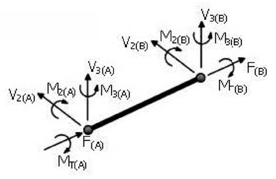
Figure 8.
12-dof infrmDBPH element [58].
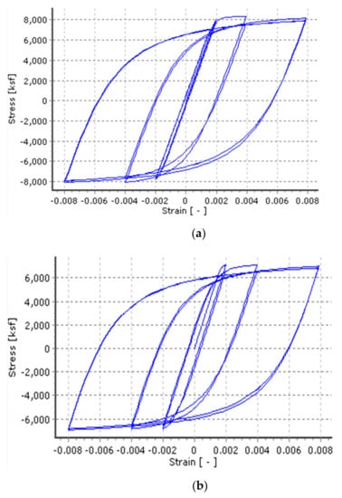
Figure 9.
Hysteresis behavior of (a) columns, and (b) beams.
The artificially generated ETEF used to perform the endurance time analysis (ETA) was Set#2 with 5% damping. Recall that ETEF Set#2 is for broad-band ground motions with magnitude 7 on rock sites. Based on Set#2’s characteristics, six real ground motions from the FEMA 440 study given in Table 3 were selected and the response spectra generated for these six ground motions and for the artificial ETEF Set#2 are shown and compared in Figure 10.
Table 3.
Selected ground motions used for IDA of the FEMA 440 steel frame.
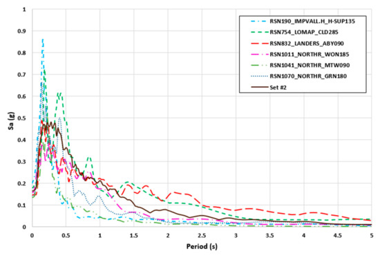
Figure 10.
Response spectra of the six FEMA440 ground motions and ETEF Set#2.
For the purpose of comparison, the steel frame was analyzed using both the endurance time and incremental dynamic analysis (IDA) methods. The IDA was performed using a 3/2 fixed scaling factor increment, starting from 2/3 the magnitude of the ground motion, and scaled up five times to 5.0625. Thus, to obtain the results for six ground motions, a total of 36 time history analyses were performed. Table 4 presents the run time and output file size for the above-mentioned analyses as performed by a computer with the Intel(R) Core(TM) i7 CPU M330 with a 2.13 GHz processor and 16.00 GB installed memory (RAM) on a 32-bit operating system. Additionally, given in the table is a comparison of the total time required to perform the entire IDA for this three-story steel frame using the six ground motions with the time needed to perform just one time history analysis using the endurance time analysis method in conjunction with ETEF Set#2.
Table 4.
Comparison of IDA and ETA computation time and output file sizes.
The locations of plastic hinges at the performance level of collapse prevention (CP) obtained using endurance time analysis are shown in Figure 11. Note, that the use of the ETA method with ETEF Set#2 successfully identifies the weak story in the structure.
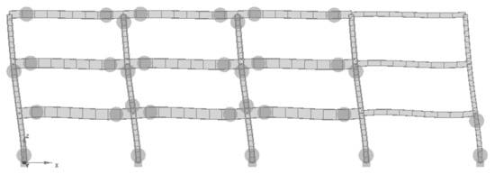
Figure 11.
Plastic hinge formation at 103.7 s (Performance Level—CP).
The base shear–roof displacement response of the frame together with its envelope curve (a curve joining the peak points of each hysteresis loop) obtained using the IDA method when the frame is subjected to the Landers earthquake is shown in Figure 12. The base shear–roof displacement response and the corresponding envelope curve of the same frame analyzed using the ETA method with ETEF Set#2 is given in Figure 13. In Figure 14, the six envelope curves obtained using the IDA method for the six ground motions are compared with that obtained using the ETA method and in Figure 15, the average of these six IDA envelope curves is compared with the ETA envelope curve. As can be seen, a good correlation between the results obtained using the IDA method (which is more computationally intensive and time-consuming to perform) and the ETA method is observed.
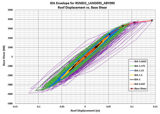
Figure 12.
Base shear versus roof displacement response and IDA envelope for RSN832 Landers.
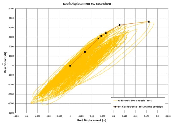
Figure 13.
Base shear versus roof displacement response and the ETA envelope for ETEF Set#2.
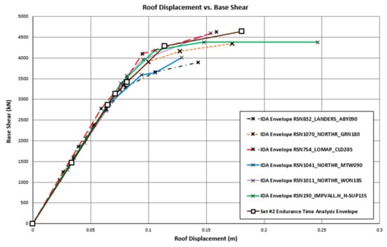
Figure 14.
Comparison of IDA and ETA envelopes.
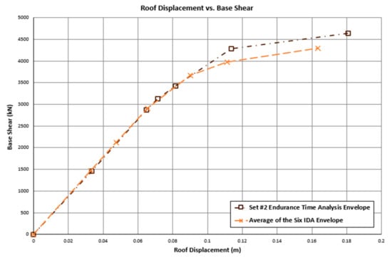
Figure 15.
Comparison of the average IDA Envelope with the ETA Envelope.
5.2. Single-Column Bridge Bent
A full-scale single-column bridge bent was tested on a shaking table by Schoettler et al. [63] at the University of California, San Diego. The full-scale cantilever bridge bent, which was 7.32 m tall and 1.22 m wide, was designed to be flexural dominated based on the seismic provisions of the Caltrans Bridge Design Specifications [64]. A plastic hinge was expected to form right above the fixed support when the bridge bent was subjected to strong ground motion. A cast-in-place concrete block was placed at the top of the test column to represent the weight of the superstructure that would take the column to the nonlinear phase.
The compressive strength of concrete used was 24.6 MPa and the elastic modulus was 23.5 GPa. The column was reinforced by eighteen ASTM A706 Grade 60 #11 in the longitudinal direction as shown in Figure 16a. The concrete cover was 51 mm. The properties of the steel reinforcement used are summarized in Table 5.
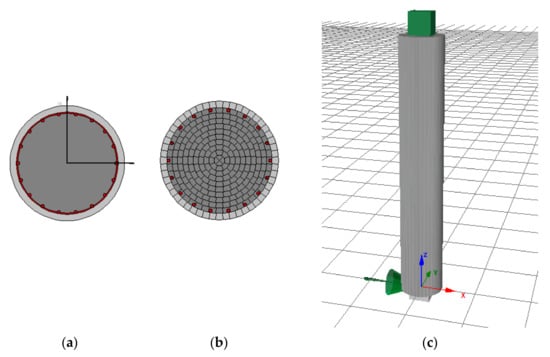
Figure 16.
(a) Bridge bent cross-section, (b) SeismoStruct modeling of the cross-section, and (c) SeismoStruct 3D rendering of the bent.
Table 5.
Steel reinforcement properties [63].
The concrete bridge bent was modeled in SeismoStruct as shown in Figure 16b,c using the inelastic force-based fiber element (infrmFB). This is a 3-D element capable of capturing material and geometry nonlinearities. The cross-section of the bent was modeled using 2682 elements, and nine elements were used along the longitudinal direction of the bent. Thus, a total of 24,138 elements were used to model the entire structure. The cross-section of stress-strain behavior was computed by integrating the uniaxial material nonlinear response of each fiber that constitutes the section.
The material models used were the Menegotto–Pinto steel model [60] described earlier, and the Mander et al. [65] nonlinear concrete material model. The Mander et al. concrete model is a uniaxial nonlinear constant confinement model proposed by Madas [66], using the stress-strain relationship proposed by Menegotto and Pinto [60] and the cyclic hysteresis loop presented by Martinez-Rueda and Elnashai [67]. The model’s uniaxial hysteresis loops for reinforcing steel and concrete are shown in Figure 17.
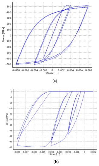
Figure 17.
Hysteresis material model for (a) reinforcing steel, and (b) concrete.
In analyzing this bridge bent using the endurance time analysis method (ETA), the artificially generated ETEF for Earthquake Set#1a was used. Recall that Earthquake Set#1a is a set of broad-band ground motions with magnitude 7 on soil sites. Using Earthquake Set#1a’s ground motion characteristics, six real ground motions used in the PEER 2015 study [68] as given in Table 6 were selected and used to perform time history analysis (THA) on the same bridge bent. The results obtained using these two methods of analysis are then compared. The ground motions used in the PEER 2015 report and the artificially generated Set#1a ETEF used in the present study are shown in Figure 18. The corresponding response spectra are shown in Figure 19.
Table 6.
Ground Motions used in the PEER 2015 Study [68].
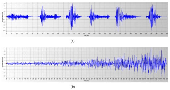
Figure 18.
(a) Six sequentially applied ground motions, and (b) ETEF Set#1a.
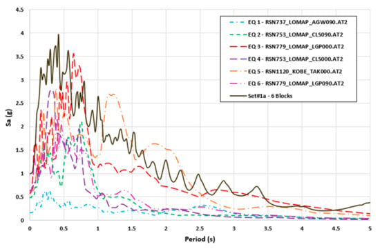
Figure 19.
Response spectra of six ground motions and ETEF Set#1a.
In the PEER 2015 study, time history analysis (THA) was performed on the bridge column when it was subjected to the six ground motions applied sequentially. The sequence of applied earthquakes was designed to push the column into the nonlinear range. The same column was then analyzed using the ETA method with ETEF Set#1a. A comparison of the run time and output file size for these two analyses is given in Table 7. Both analyses were performed by a computer with the Intel(R) Core(TM) i7 CPU M330, with a 2.13 GHz processor and 16.00 GB installed memory (RAM) on a 32-bit operating system. As can be seen in the table, the analysis performed using ETA can be accomplished with a much shorter run time and smaller file size.
Table 7.
Comparison of THA and ETA computation time and output file size.
In Table 8, the chord rotation that corresponds to the performance level of immediate occupancy (IO), life safety (LS) and collapse prevention (CP) as defined in ASCE 41-17 [69] as well as values for concrete cover damage and spalling as given by Priestley [70] and concrete core damage as given by Ribeiro et al. [71] are summarized for both analysis methods. As can be seen, good correlation is observed.
Table 8.
Summary of performance criteria.
Figure 20 shows the location of the plastic hinge of the bent when it was subjected to ETEF Set#1a, which compares well with the reported test results. The base shear–tip displacement responses of the bent when it was subjected to the six real ground motions applied sequentially (and analyzed using THA) and when it was subjected to the single ETEF Set#1a (analyzed using ETA) are shown in Figure 21 and Figure 22, respectively. For the purpose of comparison, the maximum displacement envelopes obtained using the two analysis methods (THA versus ETA) are shown in Figure 23. A good correlation is observed.
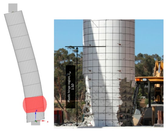
Figure 20.
Deflected shape and plastic hinge formation near the bottom of the bridge bent.
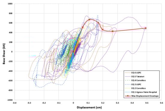
Figure 21.
Base shear versus tip displacement response and envelope curve for the six ground motions applied sequentially.
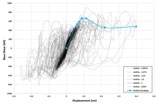
Figure 22.
Base shear versus tip displacement response and envelope curve for ETEF Set#1a.
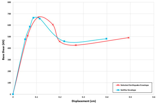
Figure 23.
Comparison of THA and ETA maximum displacement envelopes.
From this example, it can be seen that ETA when used with the proposed artificially generated ETEF can produce good and reliable results when compared to the more computationally intensive THA using all six ground motions. Considering the much shorter computation time and smaller output file size, the use of ETA with the proper artificially generated ETEF to assess the seismic performance of structures is justified.
6. Summary
In this paper, endurance time excitation functions (ETEFs) developed from three sets of real ground motions that can be used for endurance time analysis (ETA) are described. The steps involved in generating these ETEFs are summarized as follows:
- (1)
- Select ground motions that are representative of the site conditions.
- (2)
- Perform wavelet analysis on these ground motions to identify their frequency contents, the dominant frequencies, windows of frequencies (frequencies that are within 10% of the dominant frequencies) and the corresponding time durations.
- (3)
- Perform statistical analysis to determine the frequency range that contains at least 90% of the frequency contents of these ground motions and to identify the 90 percentile time duration for the windows of the frequencies.
- (4)
- Generate artificial excitation with a time duration equal to that obtained in Step 3 using the geometric mean of the selected set of ground motions as the target response spectrum.
- (5)
- Correct the frequency contents of the artificial earthquake generated in Step 4 based on data obtained in Step 3 using the sixth-order Type 1 Chebyshev filter function.
- (6)
- Regenerate the artificial excitation and intensify it using a block-shaped intensifying envelope.
The ETEF obtained can then be used as excitation input to conduct ETA to determine the nonlinear responses of structures. When compared to the incremental dynamic analysis (IDA) and time history analysis (THA) using multiple earthquakes, ETA is shown to be less computationally intensive and less time-consuming, yet it is capable of producing comparable results.
Two examples, a multi-story multi-bay steel frame and a single-column bridge bent, were given to demonstrate the accuracy and effectiveness of ETA using the proposed ETEF.
Supplementary Materials
The following supporting information can be downloaded at: https://www.mdpi.com/article/10.3390/civileng4030043/s1, Table S1: Artificial Excitations.
Author Contributions
Conceptualization, E.M.L.; Data curation, M.M.; Formal analysis, M.M.; Methodology, M.M. and E.M.L.; Project administration, E.M.L.; Supervision, E.M.L.; Validation, M.M. and E.M.L.; Visualization, M.M.; Writing—original draft, M.M.; Writing—review and editing, E.M.L. All authors have read and agreed to the published version of the manuscript.
Funding
This research received no external funding.
Data Availability Statement
The acceleration data for the three artificial excitations presented in Table S1 are available in the Supplementary Materials section of this paper.
Acknowledgments
The authors would like to acknowledge the reviewers for providing them with valuable and insightful comments. We also want to acknowledge the Department of Civil and Environmental Engineering at Syracuse University for providing the first author with financial support in the form of research and teaching assistantships.
Conflicts of Interest
The authors declare no conflict of interest.
Appendix A. Earthquake Data Set (Adapted from Baker et al. [49])
| Earthquake Set#1a | Earthquake Set#1b | Earthquake Set#2 | ||||||
|---|---|---|---|---|---|---|---|---|
| RSN | Earthquake (Station) | M | RSN | Earthquake (Station) | M | RSN | Earthquake (Station) | M |
| 231 | Mammoth Lakes-01 (Long Valley Dam, Upr L Abut) | 6.1 | 915 | Big Bear-01 (Lake Cachulla) | 6.5 | 72 | San Fernando (Lake Hughes #4) | 6.6 |
| 1203 | Chi-Chi, Taiwan (CHY036) | 7.6 | 935 | Big Bear-01 (Snow Creek) | 6.5 | 769 | Loma Prieta (Gilroy Array #6) | 6.9 |
| 829 | Cape Mendocino (Rio Dell Overpass—FF) | 7.0 | 761 | Loma Prieta (Fremont, Emerson Court) | 6.9 | 1165 | Kocaeli, Turkey (Izmit) | 7.5 |
| 169 | Imperial Valley-06 (Delta) | 6.5 | 190 | Imperial Valley-06 (Superstition Mtn Camera) | 6.5 | 1011 | Northridge-01 (LA-Wonderland Ave. | 6.7 |
| 1176 | Kocaeli, Turkey (Yarimca) | 7.5 | 2008 | CA/Baja Border Area (El Centro Array #7) | 5.3 | 164 | Imperial Valley-06 (Cerro Prieto) | 6.5 |
| 163 | Imperial Valley-06 (Calipatria Fire Sta.) | 6.5 | 552 | Chalfant Valley-02 (Lake Crowley, Sherhorn Res.) | 6.2 | 1787 | Hector Mine (Hector) | 7.1 |
| 1201 | Chi-Chi, Taiwan (CHY034) | 7.6 | 971 | Northridge-01 (Elizabeth Lake) | 6.7 | 80 | San Fernando (Pasadena-Old Seis. Lab.) | 6.6 |
| 1402 | Chi-Chi, Taiwan (NST) | 7.6 | 1750 | Northwest China-02 (Jiashi) | 5.9 | 1618 | Duzce, Turkey (Lamont 531) | 7.1 |
| 1158 | Kocaeli, Turkey (Duzce) | 7.5 | 268 | Victoria, Mexico (SAHOP Casa Flores) | 6.3 | 1786 | Hector Mine (Heart Bar State Park) | 7.1 |
| 281 | Trinidad (Rio Dell Overpass, E Ground) | 7.2 | 2003 | CA/Baja Border Area (Calexico Fire Station) | 5.3 | 1551 | Chi-Chi, Taiwan (TCU138) | 7.6 |
| 730 | Spitak, Armenia (Gukasian) | 6.8 | 668 | Whittier Narrows-01 (Norwalk, Imp Hwy S Grnd) | 6.0 | 3507 | Chi-Chi, Taiwan (TCU129) | 6.3 |
| 768 | Loma Prieta (Gilroy Array #4) | 6.9 | 88 | San Fernando (Santa Felita Dam Outlet) | 6.6 | 150 | Coyote Lake (Gilroy Array #6) | 5.7 |
| 1499 | Chi-Chi, Taiwan (TCU060) | 7.6 | 357 | Coalinga-01 (Parkfield, Stone Corral 3E) | 6.4 | 572 | Taiwan SMART1(45) (SMART1 E02) | 7.3 |
| 266 | Victoria, Mexico (Chihuahua) | 6.3 | 188 | Imperial Valley-06 (Plastic City) | 6.5 | 285 | Irpinia, Italy-01 (Bagnoli Irpinio) | 6.9 |
| 761 | Loma Prieta (Fremont—Emerson Ct.) | 6.9 | 22 | El Alamo (El Centro Array #9) | 6.8 | 801 | Loma Prieta (San Jose-Santa Teresa Hills) | 6.9 |
| 558 | Chalfant Valley-02 (Zack Brothers Ranch) | 6.2 | 762 | Loma Prieta (Fremont, Mission San Jose) | 6.9 | 286 | Irpinia, Italy-01 (Bisaccia) | 6.9 |
| 1543 | Chi-Chi, Taiwan (TCU118) | 7.6 | 535 | N. Palm Springs (San Jacinto, Valley Cementary) | 6.1 | 1485 | Chi-Chi, Taiwan (TCU045) | 7.6 |
| 2114 | Denali, Alaska (TAPS Pump Sta. #10) | 7.9 | 951 | Northridge-01 (Bell Gardens, Jaboneria) | 6.7 | 1161 | Kocaeli, Turkey (Gebze) | 7.5 |
| 179 | Imperial Valley-06 (El Centro Array #4) | 6.5 | 2465 | Chi Chi, Taiwan (CHY034) | 6.2 | 1050 | Northridge-01 (Pacoima Dam, downstr) | 6.7 |
| 931 | Big Bear-01 (San Bernardino, E and Hospitality) | 6.5 | 456 | Morgan Hill (Gilroy Array #2) | 6.2 | 2107 | Denali, Alaska (Carlo, temp) | 7.9 |
| 900 | Landers (Yermo Fire Sta.) | 7.3 | 2009 | CA/Baja Border Area (Holtville Post Office) | 5.3 | 1 | Helena, Montana-01 (Carroll College) | 6.0 |
| 1084 | Northridge-01 (Sylmar—Converter Station) | 6.7 | 470 | Morgan Hill (San Juan Bautista, 24 Polk St.) | 6.2 | 1091 | Northridge-01 (Vasquez Rocks Park) | 6.7 |
| 68 | San Fernando (LA-Hollywood Stor FF) | 6.6 | 216 | Livermore-01 (Tracy, Sewage Treatment Plant) | 5.8 | 1596 | Chi-Chi, Taiwan (WNT) | 7.6 |
| 527 | N. Palm Springs (Morongo Valley) | 6.1 | 2664 | Chi-Chi, Taiwan-03 (TCU145) | 6.2 | 771 | Loma Prieta (Golden Gate Bridge) | 6.9 |
| 776 | Loma Prieta (Hollister—South and Pine) | 6.9 | 522 | N. Palm Springs (Indio) | 6.1 | 809 | Loma Prieta (UCSC) | 6.9 |
| 1495 | Chi-Chi, Taiwan (TCU055) | 7.6 | 131 | Friuli, Italy (Codroipo) | 5.9 | 265 | Victoria, Mexico (Cerro Prieto) | 6.3 |
| 1194 | Chi-Chi, Taiwan (CHY025) | 7.6 | 964 | Northridge-01 (Compton, Castlegate St.) | 6.7 | 1078 | Northridge-01 (Santa Susana Ground) | 6.7 |
| 161 | Imperial Valley-06 (Brawley Airport) | 6.5 | 460 | Morgan Hill (Gilroy Array #7) | 6.2 | 763 | Loma Prieta (Gilroy, Gavilan Coll.) | 6.9 |
| 1236 | Chi-Chi, Taiwan (CHY088) | 7.6 | 920 | Big Bear-01 (Northshore, Salton Sea Pk HQ) | 6.5 | 1619 | Duzce, Turkey (Mudurnu) | 7.1 |
| 1605 | Duzce, Turkey (Duzce) | 7.1 | 933 | Big Bear-01 (Seal Beach, Office Bldg) | 6.5 | 957 | Northridge-01 (Burbank, Howard Rd.) | 6.7 |
| 1500 | Chi-Chi, Taiwan (TCU061) | 7.6 | 214 | Livermore-01 (San Ramon, Eastman Kodak) | 5.8 | 2661 | Chi-Chi, Taiwan-03 (TCU138) | 6.2 |
| 802 | Loma Prieta (Saratoga—Aloha Ave.) | 6.9 | 328 | Coalinga-01 (Parkfield, Cholame 3W) | 6.4 | 3509 | Chi-Chi, Taiwan-06 (TCU138) | 6.3 |
| 6 | Imperial Valley-02 (El Centro Array #9) | 7.0 | 122 | Friuli, Italy (Codroipo) | 6.5 | 810 | Loma Prieta (USCS Lick Obser.) | 6.9 |
| 2656 | Chi-Chi, Taiwan-03 (TCU123) | 6.2 | 2473 | Chi Chi, Taiwan-03 (CHY047) | 6.2 | 765 | Loma Prieta (Gilroy Array #1) | 6.9 |
| 982 | Northridge-01 (Jensen Filter Plant) | 6.7 | 757 | Loma Prieta (Dumbarton Bridge W. End FF) | 6.9 | 1013 | Northridge-01 (LA Dam) | 6.7 |
| 2509 | Chi-Chi, Taiwan-03 (CHY104) | 6.2 | 705 | Whittier Narrows-01 (W. Covina, S. Orange Ave. | 6.0 | 1012 | Northridge-01 (LA00) | 6.7 |
| 800 | Loma Prieta (Salinas—John and Work) | 6.9 | 247 | Mammoth Lakes-06 (Bishop, Paradise Lodge) | 5.9 | 1626 | Sitka, Alaska (Sitka Obser.) | 7.7 |
| 754 | Loma Prieta (Coyote Lake Dam, Downst) | 6.9 | 340 | Coalings-01 (Parkfield, Fault Zone 16) | 6.4 | 989 | Northridge-01 (LA, Chalon Rd.) | 6.7 |
| 1183 | Chi-Chi, Taiwan (CHY008) | 7.6 | 3275 | Chi-Chi, Taiwan (CHY036) | 6.3 | 748 | Loma Prieta (Belmont-Envirotech) | 6.9 |
| 3512 | Chi-Chi, Taiwan-06 (TCU141) | 6.3 | 604 | Whittier Narrows-01 (Canoga Park, Topanga Can) | 6.0 | 1549 | Chi-Chi, Taiwan (TCU129) | 7.6 |
RSN = Record Sequence Number (Next Generation Attenuation, PEER), M = magnitude.
References
- National Research Council. Improved Seismic Monitoring-Improved Decision-Making: Assessing the Value of Reduced Uncertainty; National Academies Press: Washington, DC, USA, 2006. [Google Scholar]
- ASCE/SEI 7-22; Minimum Design Loads and Associated Criteria for Buildings and Other Structures. American Society of Civil Engineers: Reston, VA, USA, 2022.
- International Code Council. International Building Code; International Code Council: Country Club Hills, IL, USA, 2021. [Google Scholar]
- Kalakan, E.; Kunnath, S. Assessment of current nonlinear static procedures for seismic evaluation of buildings. Eng. Struct. 2007, 29, 305–316. [Google Scholar] [CrossRef]
- Jalayer, F.; Cornell, C. Alternative non-linear demand estimation methods for probability-based seismic assessments. Earthq. Eng. Struct. Dyn. 2009, 38, 951–972. [Google Scholar] [CrossRef]
- Vamvatsikos, D.; Cornell, C. Incremental dynamic analysis. Earthq. Eng. Struct. Dyn. 2002, 31, 491–514. [Google Scholar] [CrossRef]
- Mackie, K.R.; Stojadinović, B. Comparison of incremental dynamic, cloud, and stripe methods for computing probabilistic seismic demand models. In Proceedings of the Structures Congress 2005: Metropolis and Beyond, New York, NY, USA, 20–24 April 2005; p. 11. [Google Scholar]
- Estekanchi, H.E.; Vafaei, A.; Sadegh, A.M. Endurance time method for seismic analysis and design of structures. Sci. Iran. 2004, 11, 361–370. [Google Scholar]
- Estekanchi, H.E.; Valamanesh, V.; Vafai, A. Application of endurance time method in linear seismic analysis. Eng. Struct. 2007, 29, 2551–2562. [Google Scholar] [CrossRef]
- Valamanesh, V.; Estekanchi, H.E.; Vafai, A. Characteristics of second generation endurance time acceleration functions. Sci. Iran. 2010, 7, 53–61. [Google Scholar]
- Estekanchi, H.E.; Vafai, A.; Valamanesh, V.; Mirzaee, A.; Nozari, A.; Bazmuneh, A. Recent advances in seismic assessment of structures by endurance time method. In Proceedings of the US–Iran–Turkey Seismic Workshop-Seismic Risk Management in Urban Areas, Istanbul, Turkey, 14–16 December 2011; pp. 289–301. [Google Scholar]
- Riahi, H.T.; Estekanchi, H.E.; Vafai, A. Endurance time method-application in nonlinear seismic analysis of single degree of freedom systems. J. Appl. Sci. 2009, 9, 1817–1832. [Google Scholar] [CrossRef]
- Estekanchi, H.E.; Riahi, H.T.; Vafai, A. Endurance time method: Exercise test applied to structures. In Proceedings of the 14th World Conference on Earthquake Engineering, Beijing, China, 12–17 October 2008; p. 8. [Google Scholar]
- Estekanchi, H.E.; Riahi, H.T.; Vafai, A. Endurance Time method in seismic assessment of steel frames. Eng. Struct. 2011, 33, 2535–2546. [Google Scholar] [CrossRef]
- Hariri-Ardebili, M.A.; Zarringhalam, Y.; Mirtaheri, M.; Yahyai, M. Nonlinear Seismic Response of Steel Concentrically Braced Frames Using Endurance Time Analysis Method. J. Civ. Eng. Archit. 2011, 5, 847–855. [Google Scholar]
- Valamanesh, V.; Estekanchi, H.E. Endurance time method for multi-component analysis of steel elastic moment frames. Sci. Iran. 2011, 18, 139–149. [Google Scholar] [CrossRef]
- Alembagheri, M.; Estekanchi, H.E. Seismic assessment of unanchored steel storage tanks by endurance time method. Earthq. Eng. Eng. Vib. 2011, 10, 591–603. [Google Scholar] [CrossRef]
- Tavazo, H.; Estekanchi, H.E.; Kaldi, P. Endurance time method in the linear seismic analysis of shell structures. Int. J. Civ. Eng. 2012, 10, 169–178. [Google Scholar]
- Zeinoddini, M.; Nikoo, H.M.; Estekanchi, H.E. Endurance Wave Analysis (EWA) and its application for assessment of offshore structures under extreme waves. Appl. Ocean Res. 2012, 37, 98–110. [Google Scholar] [CrossRef]
- Valamanesh, V.; Estekanchi, H.E.; Vafai, A.; Ghaemian, M. Application of the endurance time method in seismic analysis of concrete gravity dams. Sci. Iran. 2011, 18, 326–337. [Google Scholar] [CrossRef]
- Hariri-Ardebili, M.A.; Sattar, S.; Estekanchi, H.E. Performance-based seismic assessment of steel frames using endurance time analysis. Eng. Struct. 2014, 69, 216–234. [Google Scholar] [CrossRef]
- Shirkhani, A.; Mualla, I.H.; Shabakhty, N.; Mousavi, S.R. Behavior of steel frames with rotational friction dampers by endurance time method. J. Constr. Steel Res. 2015, 107, 211–222. [Google Scholar] [CrossRef]
- Basim, M.C.; Estekanchi, H.E. Application of endurance time method in performance-based optimum design of structures. Struct. Saf. 2015, 56, 52–67. [Google Scholar] [CrossRef]
- Foyouzat, M.A.; Estekanchi, H.E. Application of rigid-perfectly plastic spectra in improved seismic response assessment by Endurance Time method. Eng. Struct. 2016, 111, 24–35. [Google Scholar] [CrossRef]
- Mashayekhi, M.; Estekanchi, H.E.; Vafai, H.; Mirfarhadi, S.A. Development of hysteretic energy compatible endurance time excitations and its application. Eng. Struct. 2018, 177, 753–769. [Google Scholar] [CrossRef]
- Li, S.; Liu, K.; Liu, X.; Zhai, C.; Xie, F. Efficient structural seismic performance evaluation method using improved endurance time analysis. Earthq. Eng. Eng. Vib. 2019, 18, 795–809. [Google Scholar] [CrossRef]
- Hasani, H.; Golafshani, A.; Estekanchi, H.E. Seismic performance evaluation of jacket-type offshore platforms using endurance time method considering soil-pile-superstructure interaction. Sci. Iran. 2017, 24, 1843–1854. [Google Scholar] [CrossRef]
- Bai, J.; Jin, S.; Zhao, J.; Sun, B. Seismic performance evaluation of soil-foundation-reinforced concrete frame systems by endurance time method. Soil Dyn. Earthq. Eng. 2019, 118, 47–51. [Google Scholar] [CrossRef]
- Sarcheshmehpour, M.; Estekanchi, H.E.; Ghannad, M.A. Optimum placement of supplementary viscous dampers for seismic rehabilitation of steel frames considering soil–structure interaction. Struct. Des. Tall Spec. Build. 2020, 29, e1682. [Google Scholar] [CrossRef]
- Shirkhani, A.; Farahmand Azar, B.; Charkhtab Basim, M.; Mashayekhi, M. Performance-based optimal distribution of viscous dampers in structure using hysteretic energy compatible endurance time excitations. Int. J. Numer. Methods Civ. Eng. 2021, 5, 46–55. [Google Scholar] [CrossRef]
- Shirkhani, A.; Farahmand Azar, B.; Charkhtab Basim, M. Seismic loss assessment of steel structures equipped with rotational friction dampers subjected to intensifying dynamic excitations. Eng. Struct. 2021, 238, 112233. [Google Scholar] [CrossRef]
- Guo, A.; Shen, Y.; Bai, J.; Li, H. Application of the endurance time method to the seismic analysis and evaluation of highway bridges considering pounding effects. Eng. Struct. 2017, 131, 220–230. [Google Scholar] [CrossRef]
- Ghaffari, E.; Estekanchi, H.E.; Vafai, A. Application of endurance time method in seismic analysis of bridges. Sci. Iran. 2020, 27, 1751–1761. [Google Scholar] [CrossRef]
- He, H.; Wei, K.; Zhang, J.; Qin, S. Application of endurance time method to seismic fragility evaluation of highway bridges considering scour effect. Soil Dyn. Earthq. Eng. 2020, 136, 106243. [Google Scholar] [CrossRef]
- Pang, Y.; Cai, L.; He, W.; Wu, L. Seismic assessment of deep water bridges in reservoir considering hydrodynamic effects using endurance time analysis. Ocean Eng. 2020, 198, 106846. [Google Scholar] [CrossRef]
- Mirfarhadi, S.A.; Estekanchi, H.E. Value based seismic design of structures using performance assessment by the endurance time method. Struct. Infrastruct. Eng. 2020, 16, 1397–1415. [Google Scholar] [CrossRef]
- Mohsenian, V.; Hajirasouliha, I.; Nikkhoo, A. Multi-level Response Modification Factor Estimation for Steel Moment-Resisting Frames Using Endurance-Time Method. J. Earthq. Eng. 2020, 26, 4812–4832. [Google Scholar] [CrossRef]
- Xu, Q.; Xu, S.; Chen, J.; Li, J. A modified endurance time analysis algorithm to correct duration effects for a concrete gravity dam. Int. J. Geomech. 2022, 22, 04021285. [Google Scholar] [CrossRef]
- Estekanchi, H.E.; Mashayekhi, M.; Vafai, H.; Ahmadi, G.; Mirfarhadi, S.A.; Harati, M. A state-of-knowledge review on the Endurance Time Method. Structures 2020, 27, 2288–2299. [Google Scholar] [CrossRef]
- Goupillaud, P.; Grossmann, A.; Morlet, J. Cycle-octave and related transforms in seismic signal analysis. Geoexploration 1984, 23, 85–102. [Google Scholar] [CrossRef]
- Daubechies, I. Orthonormal bases of compactly supported wavelets. Commun. Pure Appl. Math. 1988, 41, 909–996. [Google Scholar] [CrossRef]
- Grossmann, A.; Morlet, J. Decomposition of Hardy functions into square integrable wavelets of constant shape. SIAM J. Math. Anal. 1984, 15, 723–736. [Google Scholar] [CrossRef]
- Misiti, M.; Misiti, Y.; Oppenheim, G.; Poggi, J.M. Wavelet Toolbox; The MathWorks Inc.: Natick, MA, USA, 1996; p. 626. Available online: http://ailab.chonbuk.ac.kr/seminar_board/pds1_files/w7_1a.pdf (accessed on 31 January 2019).
- Olhede, S.C.; Walden, A.T. Generalized morse wavelets. IEEE Trans. Signal Process. 2002, 50, 2661–2670. [Google Scholar] [CrossRef]
- Lilly, J.M.; Olhede, S.C. Higher-order properties of analytic wavelets. IEEE Trans. Signal Process. 2008, 57, 146–160. [Google Scholar] [CrossRef]
- Lilly, J.M.; Olhede, S.C. On the analytic wavelet transform. IEEE Trans. Inf. Theory 2010, 56, 4135–4156. [Google Scholar] [CrossRef]
- Lilly, J.M.; Olhede, S.C. Generalized Morse wavelets as a superfamily of analytic wavelets. IEEE Trans. Signal Process. 2012, 60, 6036–6041. [Google Scholar] [CrossRef]
- Lilly, J.M. Element analysis: A wavelet-based method for analysing time-localized events in noisy time series. Proc. R. Soc. A Math. Phys. Eng. Sci. 2017, 473, 20160776. [Google Scholar] [CrossRef] [PubMed]
- Baker, J.W.; Lin, T.; Shahi, S.K.; Jayaram, N. New Ground Motion Selection Procedures and Selected Motions for the PEER Transportation Research Program; PEER Report; 2011; 76p, Available online: https://peer.berkeley.edu/sites/default/files/baker_et_al_2011_peer_gm_report.pdf (accessed on 15 July 2019).
- Chiou, B.; Darragh, R.; Gregor, N.; Silva, W. NGA project strong-motion database. Earthq. Spectra 2008, 24, 23–44. [Google Scholar] [CrossRef]
- @RISK® 8. User’s Manual. Palisade. 2017. Available online: www.palisade.com (accessed on 25 September 2019).
- Bozdogan, H. Model selection and Akaike’s information criterion (AIC): The general theory and its analytical extensions. Psychometrika 1987, 52, 345–370. [Google Scholar] [CrossRef]
- SeismoArtif. Verification Report. Seismosoft. 2016. Available online: www.seismosoft.com (accessed on 4 March 2020).
- MATLAB® R2018b; User’s Guide; The MathWorks, Inc.: Natick, MA, USA, 2018.
- FEMA 440; Improvement of Nonlinear Static Seismic Analysis Procedures. Federal Emergency Management Agency (FEMA): Washington, DC, USA, 2005.
- Uniform Building Code; International Conference of Building Officials: Whittier, CA, USA, 1994.
- ANSI/AISC 341-22; Seismic Provisions for Structural Steel Buildings. American Institute of Steel Construction: Chicago, IL, USA, 2022.
- SeismoStruct. Verification Report. Seismosoft. 2018. Available online: www.seismosoft.com (accessed on 4 March 2020).
- Giberson, M.F. Two nonlinear beams with definitions of ductility. J. Struct. Div. 1969, 95, 137–157. [Google Scholar] [CrossRef]
- Menegotto, M.; Pinto, P.E. Method of analysis for cyclically loaded reinforced concrete plane frames including changes in geometry and non-elastic behavior of elements under combined normal force and bending. In IABSE Symposium on the Resistance and Ultimate Deformability of Structures Acted on by Well-Defined Repeated Loads; International Association for Bridge and Structural Engineering: Zurich, Switzerland, 1973; Volume 11, pp. 15–22. [Google Scholar]
- Yassin, M.H. Analysis of Prestressed Concrete Structures under Monotonic and Cyclic Loads; University of California: Berkeley, CA, USA, 1994. [Google Scholar]
- Filippou, F.C.; Popov, E.P.; Bertero, V.V. Effects of Bond Deterioration on Hysteretic Behavior of Reinforced Concrete Joints; Report No. UCB/EERC-83/19; University of California-Berkeley: Berkeley, CA, USA, 1983. [Google Scholar]
- Schoettler, M.J.; Restrepo, J.I.; Guerrini, G.; Duck, D.E.; Carrea, F. Full-Scale, Single-Column Bridge Bent Tested by Shake-Table Excitation; PEER Report 2015/02; University of California: Berkeley, CA, USA, 2015. [Google Scholar]
- Caltrans. Bridge Design Specifications; California Department of Transportation: Sacramento, CA, USA, 2004. [Google Scholar]
- Mander, J.B.; Priestley, M.J.; Park, R. Theoretical stress-strain model for confined concrete. J. Struct. Eng. 1988, 114, 1804–1826. [Google Scholar] [CrossRef]
- Madas, P.J. Advanced Modelling of Composite Frames Subject to Earthquake Loading. Ph.D. Thesis, Civil Engineering Department, Imperial College of Science, Technology and Medicine, University of London, London, UK, 1993. [Google Scholar]
- Martínez-Rueda, J.E.; Elnashai, A.S. Confined concrete model under cyclic load. Mater. Struct. 1997, 30, 139–147. [Google Scholar] [CrossRef]
- Terzic, V.; Schoettler, M.J.; Restrepo, J.I.; Mahin, S.A. Concrete Column Blind Prediction Contest 2010: Outcomes and Observations. PEER Rep. 2015, 1, 1–145. [Google Scholar]
- ASCE/SEI 41-17; Seismic Evaluation and Retrofit of Existing Buildings. American Society of Civil Engineers: Reston, VA, USA, 2017.
- Priestley, M.N. Myths and Fallacies in Earthquake Engineering, Revisited: The Ninth Mallet Milne Lecture; IUSS Press: Pavia, Italy, 2003; p. 119. [Google Scholar]
- Ribeiro, F.L.; Barbosa, A.R.; Scott, M.H.; Neves, L.C. Deterioration modeling of steel moment resisting frames using finite-length plastic hinge force-based beam-column elements. J. Struct. Eng. 2014, 141, 04014112-1. [Google Scholar] [CrossRef]


Disclaimer/Publisher’s Note: The statements, opinions and data contained in all publications are solely those of the individual author(s) and contributor(s) and not of MDPI and/or the editor(s). MDPI and/or the editor(s) disclaim responsibility for any injury to people or property resulting from any ideas, methods, instructions or products referred to in the content. |
© 2023 by the authors. Licensee MDPI, Basel, Switzerland. This article is an open access article distributed under the terms and conditions of the Creative Commons Attribution (CC BY) license (https://creativecommons.org/licenses/by/4.0/).