Abstract
Structural health monitoring (SHM) is crucial for ensuring the safety and performance of offshore platforms. SHM uses advanced sensor systems to detect and respond to negative changes in structures, improving their reliability and extending their life cycle. Model updating methods are also useful for sensitivity analysis. It is feasible to discuss and introduce established techniques for detecting damage in structures by utilizing their mode shapes. In this research, by considering reducing the stiffness of elements in the damage scenarios, we conducted simulations of the models in MATLAB, including both two-dimensional and three-dimensional structures, to update the method suggested by Wang. Wang’s method was improved to produce a sensitivity equation for the damaged structures. The sensitivity equation solution using a subset of mode shapes data was found to evaluate structural parameter changes. Comparing the updated results for Wang’s method and the suggested method in the two- and three-dimensional frames showed a noticeable modification in damage recognition. Furthermore, the suggested method can update a model containing measurement errors. Since Wang’s damage detection formulation is suitable only for 2D structures, this modified framework provides a more accurate decision-making tool for damage detection of structures, regardless of whether a 2D or 3D formulation is used.
1. Introduction
Due to distinct reasons, such as earthquakes, waves crashing, fatigue, and erosion, offshore platforms are faced with some changes in their structural properties, which can cause structural failure, people’s deaths, and economic damage [1]. Thus, structural safety and performance require early detection, monitoring, and analysis of the damaged structure. Different methods have been developed to identify the damage location and severity using non-destructive tests and detection algorithm responses [2]. According to the damaging effect, the damage detection algorithms can lead to a detectable change in a structure’s response [3].
There are generally two methods used to update the trends in structural health monitoring: applying forces or stresses and measuring the structural response. Damage detection using dynamic data has more advantages in comparison with static techniques, which can be more sensitive to changes in structural parameters and structural damage [4]. The dynamic characteristics of a structure, such as its mass, stiffness, and damping, can vary because of damage. As a result, damage detection techniques often rely on changes in these characteristics, as measured by modal data, such as natural frequencies, mode shapes, and damping ratios. In practice, natural frequencies can be measured more accurately than mode shapes and are, therefore, often used to update structural models [5]. However, changes in natural frequencies alone do not provide detailed information about the location or extent of damage. Therefore, utilizing mode shape data is considered to be a more valuable approach for model updating, despite the mathematical and practical challenges that it poses [6]. Modal data covering the natural frequencies and the mode shapes have been considered by researchers in recent decades.
Regarding the response, updating techniques can be classified into methods based on the mode and response. Updating a technical model based on the mode involves obtaining modal properties, which are given by indirectly measured frequency response function (FRF) data. Structural parameters are updating techniques that are applied using direct methods or iterative approaches [7,8]. A straightforward method for calibrating structural models involves adjusting the mass and stiffness parameters to match the numerical data to the measured modal data [9]. However, these changes may not be easily interpreted in terms of physical changes to the structure. An iterative updating approach that uses experimental data or frequency response function (FRF) data and techniques for updating finite element (FE) models to account for sensitivity may be required to better understand the effects of damage on a structure [10,11,12,13].
Detecting damage using experimental modal data [14] can be difficult due to noise and limited nodal points. There are different methods to address this issue, such as using the imperialist competitive optimization algorithm with damage functions and incorporating variable widths and weights. Another approach [15] involves combining incomplete modal data with sparse regularization techniques to improve the accuracy and robustness of damage identification. This method does not require sensitivity analysis or complete modal data and uses a new goal function. Structural damage is detected by using mode shape changes or the mode shape itself. Wang et al. [16] undertook a sensitivity analysis of the structural parameters. They also achieved dynamic modification directly and indirectly through modal data analysis. Kim and Stubbs [17] presented an algorithm for identifying structural damage in jacket offshore structures using few-mode shapes. Ren et al. [18] used mode shape data to locate and quantify structural damage. They proposed using sensitivity equations that involve all mode shapes of the undamaged and damaged structures. However, the need for complete mode shape data can be a limitation in structures with a high degree of freedom, making it difficult to apply the method in real-world scenarios. Lee et al. [19] used the cross-modal method as a reliable proposed method to recognize the damage in jacket offshore platforms when incomplete modal data is available.
Shahsavari et al. [20] undertook a mode shape analysis with the likelihood ratio (LR) test to specify damage. Wang et al. [21] introduced the kriging model as a secondary model to optimize by frequency response function instead of focusing just on the one FE model repeatedly. Umar et al. [22] remarked on a new response surface methodology (RSM), which used both the natural frequencies and mode shapes to upgrade the damage recognition.
Hariri-Ardebili et al. [23] coupled a polynomial chaos expansion metamodel and modal analysis to find the most vulnerable areas of arch dams in an efficient way. Dahak et al. [24] declared an approach based on normalized natural frequencies using experimental data in order to recognize damage in a cantilever beam. Khatir et al. [25] achieved a new method for the determination of cracks, which simultaneously investigates changes from measured frequencies experimentally and by using particle swarm optimization.
Model updating methods use the modal parameters elicited from vibration data in the structures, which were measured before and after damage. In order to distinguish the damage intensity in structures, Park et al. [26] presented a damage intensity function to clarify the relationship between damage intensity and multiple-per-revolution (MPR) changes for the baseline model. Schacht et al. [27] produced a modified method for damage evaluation in which the modified indexes were found using a given function combined with a genetic algorithm (GA). The identification of damage in truss and beam-like structures which was achieved using FRF data combined with optimization techniques [28], presenting the fastest solution compared with other approaches that used a GA and bat algorithm (BA) to find the location and severity of the damage.
Pérez and López [29] developed a fully functional SHM system based on spectral domain indices. They characterized a comparison between experimental data and numerical data, which led to a careful assessment of proposed spectral correlation indices (SCIs) for structural evaluation and damage identification. Khatir et al. [30] indicated one specific approach that has two steps in order to assess damage in beam-like structures using two dimensions, namely, isogeometric analysis (IGA) and finite element method besides optimization techniques. Abasi et al. [31] presented a damage identification method using the nearest neighbor search method to evaluate structures. Consequently, the nearest neighbor search method was rather strong for noisy data in comparison to the artificial neural network.
Sensitivity-based model updating can be done based on mode shape changes [32]. The accurate assessment of mode shape changes by considering unknown structural parameters is a crucial issue for updating a model. A sensitivity equation can be linear or of a higher degree. Linear sensitivity needs measurement in all freedom degrees, which is a challenging issue for real structures. Furthermore, the first-order Taylor series expansion enables the calculation of a linear formula for updating the model.
Iannelli et al. [33] researched using deep learning to identify damage in large space antennas. They explored the use of a long short-term memory neural network for the classification of various types of damage, and the results indicate successful detection. Wang ad Wu [34] suggested an enhanced version of explicit connectivity Bayesian networks for analyzing system reliability. Their approach considers multiple failure modes and the probabilistic relationships between different components.
To understand the relationship between changes in the mode shapes and structural parameters, a sensitivity equation was employed to revise the model. This equation utilizes eigenvector derivatives, and various techniques were proposed by researchers to calculate these derivatives. One method is the modal method, which is used to estimate the derivative of mode shapes based on design variables. Another method, which is called the Nelson method, is a reliable way to evaluate eigenvalue derivatives. Additionally, the Wang method, which improves upon the modal method by incorporating a quasi-static term into the eigenvector derivative equation, was shown to accelerate the convergence of the modal method [35,36,37]. Damage detection by using both modal and Wang methods leads to similar results, which were confirmed using the equation. The superiority of the Wang method is because of its better convergence [38].
In this article, a brief consideration of both standard damage recognition methods (modal and Wang’s methods) is presented. An improved model updating method based on natural frequencies combination was suggested. To enhance Wang’s method [37] for accurate damage recognition in both two-dimensional and three-dimensional frames, an updated model incorporating measurement errors and precise damage identification was employed. This update involved utilizing the natural frequency of the damaged structure to establish a more precise correlation between changes in mode shapes and structural parameters. Wang’s damage detection formula is limited to 2D structures, but this adapted framework provides a precise tool for identifying damage in structures, irrespective of their 2D or 3D formulation.
According to our detailed review in Section 1, the need for proposing a modified damage detection framework based on Wang’s model formed the backbone of the current study. Since Wang’s damage detection formulation is suitable only for 2D structures, this study was centered on extending the applicability of Wang’s model to 3D structures. Furthermore, one may note that it can be appealing to increase the accuracy of Wang’s model by adding an error metric during updating the model. To meet these two major contributions of this study, some ingredients are required, which are comprehensively described in the following.
In Section 2, the background theory of Wang’s model is introduced, along with the basis of the updating procedure. Next, assumptions for numerical simulation and the configuration of strain gauges are described briefly in Section 3 and Section 4, respectively. The application of the proposed formulation for 2D and 3D structures is demonstrated in Section 5. Finally, the major contributions and outputs of this study, in conjunction with some recommendations for future works, are described in Section 6. This research developed an improved SHM method that extends the capability of existing techniques, enabling accurate damage detection in both 2D and 3D structures, and accommodating model updates and measurement errors. This advancement can significantly enhance the reliability and effectiveness of structural health monitoring systems for offshore platforms and other structures.
2. Description of Theory and Analysis Method
2.1. Theory
This section provides a brief overview of the methods presented in Wang’s model [37] and the modal method. It also mentions the characteristic equation of eigenvalues for an undamaged structure (without damping), which is introduced by Equation (1).
In the equation provided, Knxn and Mnxn represent the structural stiffness matrix and mass matrix, respectively. The variable is the eigenvector and is the ith eigenvalue. The square of the ith natural frequency is represented by and the number of freedom degrees is represented by n. By taking the derivative of both sides of the equation, the equation can be rewritten.
The derivative of an eigenvalue can be found by multiplying Equation (2) through by , as shown in Equation (3).
where , , and give the derivatives of eigenvalues, stiffness matrix, and mass matrix, respectively. Based on the modal method, the derivative of the ith eigenvector is expressed as a series expansion of all eigenvectors:
Moreover, the factor is defined as follows:
The modal method or Fax formula is a common way to appraise the derivative of a mode shape. Wang [37] presented the modified modal method. Using Wang’s method leads to expressing the derivative of the ith mode shape as a linear combination of mode shapes, as indicated by Equation (6).
In Equation (6), the combinatory coefficients demonstrate the share of the jth mode shape, as expressed by Equation (8).
Wang’s method [37] is employed for determining the derivative of the modal shapes. In this method, the derivatives of the eigenvalues must be taken into consideration. Equation (3) serves as the sole means of evaluating the derivatives of natural frequencies in response to design variables. Accordingly, the initial evaluation of alterations in modal shapes is presented by Equation (9), wherein p constitutes a diagonal matrix of stiffness parameters.
The matrices of mass and stiffness of linear function are unknown matrices from structural parameters:
As a result, eigenvalue changes can be found as follows:
A method was developed for determining structural damage by analyzing changes in the natural frequencies. can be calculated using the following equation:
Equation (13) can be used to account the accuracy and logical value for in comparison to Equation (3). Consequently, the mode shape changes can be revealed by replacing Equation (13) in Equation (9), and thus, rewriting it as Equation (14).
The first term of Equation (14) is calculated by utilizing the damaged structure, which measures the natural frequencies, mass, stiffness, and mode shapes. Therefore, it can be utilized instead of the parametric formula of this term for updating the model.
To define the term , Equation (9) is rewritten as follows:
Since the changes in the structure’s mass matrix are minimal, even after destruction, the difference in mass can be discarded. The stiffness matrix as a function of structural parameters is depicted by Equation (17).
Matrix A, with dimensions of npxnp, is referred to as the stiffness connectivity matrix. It is a diagonal matrix, with the stiffness parameters of elements, which are represented by npx1 P-forms and P-vectors, serving as its input.
The total stiffness matrix, as stated in Equation (19), is a linear function of the stiffness parameters. Furthermore, the matrix [A] is not dependent on the matrix [P].
Expanding Equation (19) and subtracting it from Equation (17) leads to obtaining a parametric form of the total stiffness matrix, as revealed in Equation (20).
If Equation (20) is accommodated in Equation (19), the changes in the ith mode shape can depend on changes in the stiffness parameters:
Equation (22) illustrates the relationship between the strain and the displacement.
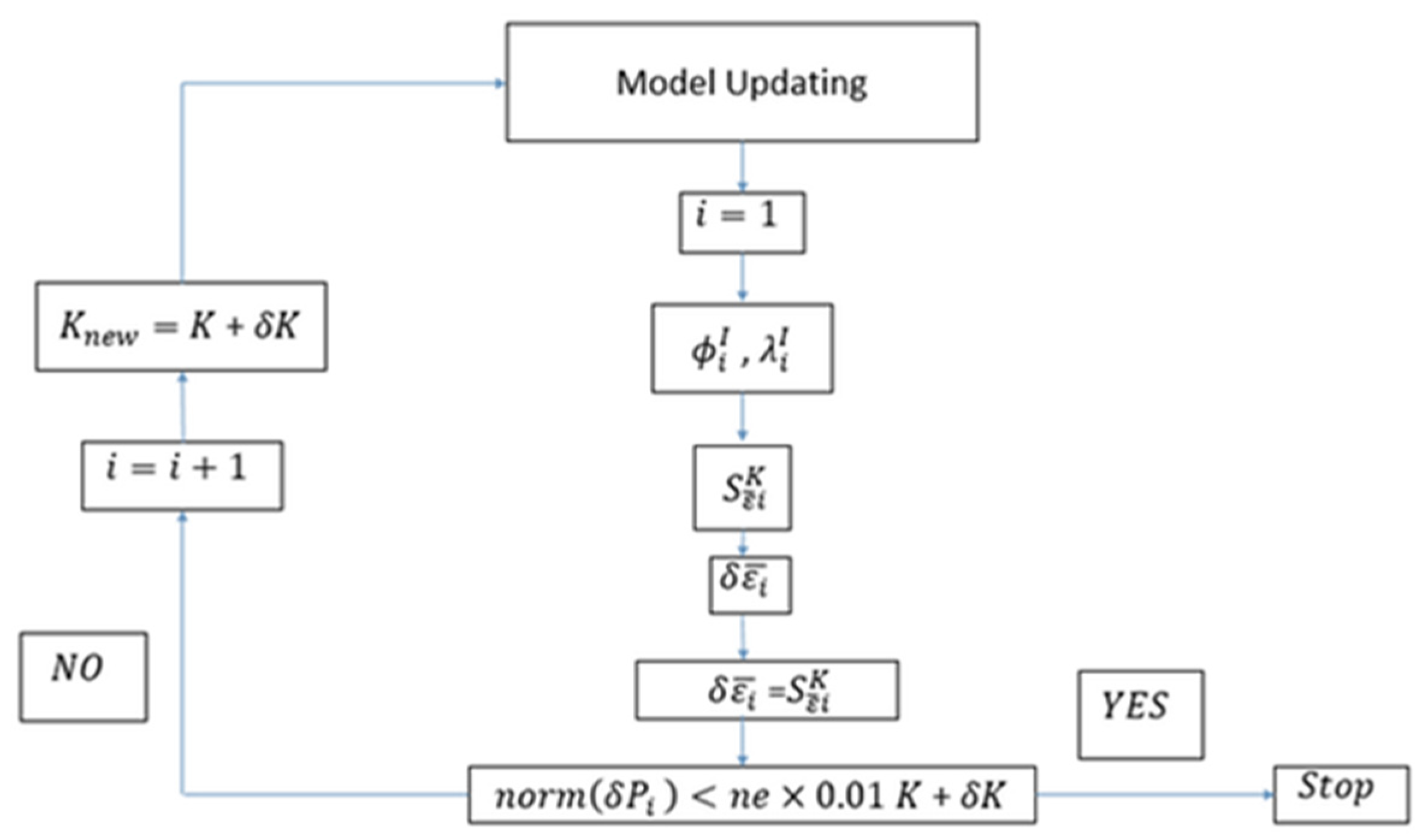
As an overview, the steps for updating the model are provided in the following flowchart (Figure 1). The purpose of updating the model is to align the predicted results of the model with actual measurements by adjusting certain key parameters. The distance between the theoretical and experimental outcomes is often measured using the mean of the least squares, and thus, updating the model can be seen as a problem of structural optimization. Since the variation of the ith mode shape is related to changes in the stiffness parameters, by altering the natural frequency and mode shape of healthy modes and measuring the strain, we can obtain changes in the diagonal matrix, including the eigenvalues of the combined stiffness matrix of the components. Finally, the structural update process is compared with the individual components. If the results are not in agreement, the process is repeated with variations in stiffness. The steps in the flowchart are as follows:
: ith eigenvector in the healthy state;
: ith eigenvalue in the healthy state;
: updated stiffness;
: stiffness variation;
: strain variation.
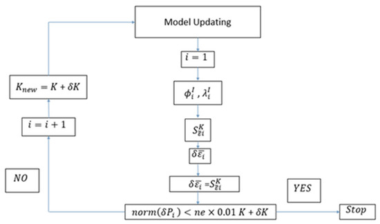
Figure 1.
Flowchart of the steps for model updating.
Figure 1.
Flowchart of the steps for model updating.
2.2. Analysis Method
In practical applications, the successful utilization of vibration information models is limited due to measurement errors. These errors can arise from factors such as noise during frequency and mode measurements of the structure being tested. Such errors have undesirable consequences, as they can lead to failures going undetected or result in excessive predictions of failure. To simulate the presence of errors and noise in the measurement process, random noise of 1% was generated using MATLAB software. This noise was then multiplied by the mode shape of the damaged structure. The noise application loop, which operated outside the failure detection loop, generated a noise matrix for each iteration. The loop ran fifty times, creating fifty noise matrices. Each time, failure detection was performed, and the average of the detected failures over fifty iterations was calculated. Additionally, the standard deviation was computed and plotted to indicate the dispersion of failure detections across the fifty noise applications. By simulating fifty measurement errors, the goal was to mimic a scenario where the structure’s response was measured fifty times in a laboratory, with failure detection performed each time. This method aimed to assess the accuracy of the approach in the presence of measurement errors.
3. Assumptions and Constraints of Numerical Modeling
In this research, we assumed that damage causes a change in the stiffness of structural elements, and this change, along with reduced flexural stiffness, applies to the structure. The proposed method links the alterations in the valid parameters to the mode shape of a structurally damaged object, as informed by the data. The stiffness matrix can be computed by adding together the stiffness matrices of the parts, as outlined in Equation (24).
Here, Kr represents the contribution of a specific part to the overall stiffness matrices, and nE stands for the number of elements. Hence, the behavior of the stiffness matrix can be rewritten as follows:
Krd symbolizes the stiffness of the rth element when it is damaged, and is a scalar multiplier that demonstrates the proportional changes in the stiffness of the rth element in both damaged and undamaged states. The fluctuation of axial rigidity is indicated by the value of , which is obtained from the truss elements. Equation (25) is utilized to modify both the bending and axial rigidities in frame elements through decomposition.
To use methods of damage identification, the response of the structure should continue to display linear behavior after a seismic load; this method supposed which analytical model of the structure should be obtained before applying this method. The linear finite element modeling for a healthy structure was monitored as a basic model update to detect parameters of structural model stiffness [26]. For verification, the simulated structure was updated with the finite element method of the structural model and the behavior of the existing model was consistent with the realistic structural model.
The proposed method’s effectiveness was examined in two models in this study. The approach was tested on a two-dimensional frame with 32 elements that underwent multiple damage scenarios. Additionally, the same method was tested on a three-dimensional frame that had 48 elements.
In the study, the mode shapes of the damaged structure were subjected to noise [14] about fifty times. Furthermore, by applying the same noise level (around 1%), the measurement error and standard deviation value were calculated. To ensure a reliable solution, several factors needed to be considered, including the type and location of the sensor, the type and location of the excitation, the quality of the measurement data (measurement error), the accuracy of the mathematical model (modeling error), and the numerical methods used.
4. Installation of the Strain Gauge
The placement of strain gauges on 2D and 3D frames depends on the specific requirements of the structure and the type of information needed for the analysis. Typically, strain gauges are placed at critical locations on the structure, such as near joints, supports, or areas susceptible to damage. For 2D frames, strain gauges are typically installed at the top and bottom of the frame, while for 3D frames, they can be placed on different faces of the structure to capture the deformations in different directions. The specific positioning of strain gauges can be determined through careful analysis and modeling of the structure to ensure the accuracy and reliability of the collected data. In this study, natural frequencies and mode shapes were acquired from sensors and applied to the damaged structure. The data was used to detect damage by using optimized equations, which improved Wang’s method. The performance and validity of this approach were verified and investigated for both 2D and 3D frames. Due to various factors that affect the detection of the structure, a limited number of sensors must be used to measure strains, including determining the sensor location for access to different sides of the structure and measuring capabilities. Hence, the sensor location was determined based on the element’s strain energy density, which is calculated using Equation (26).
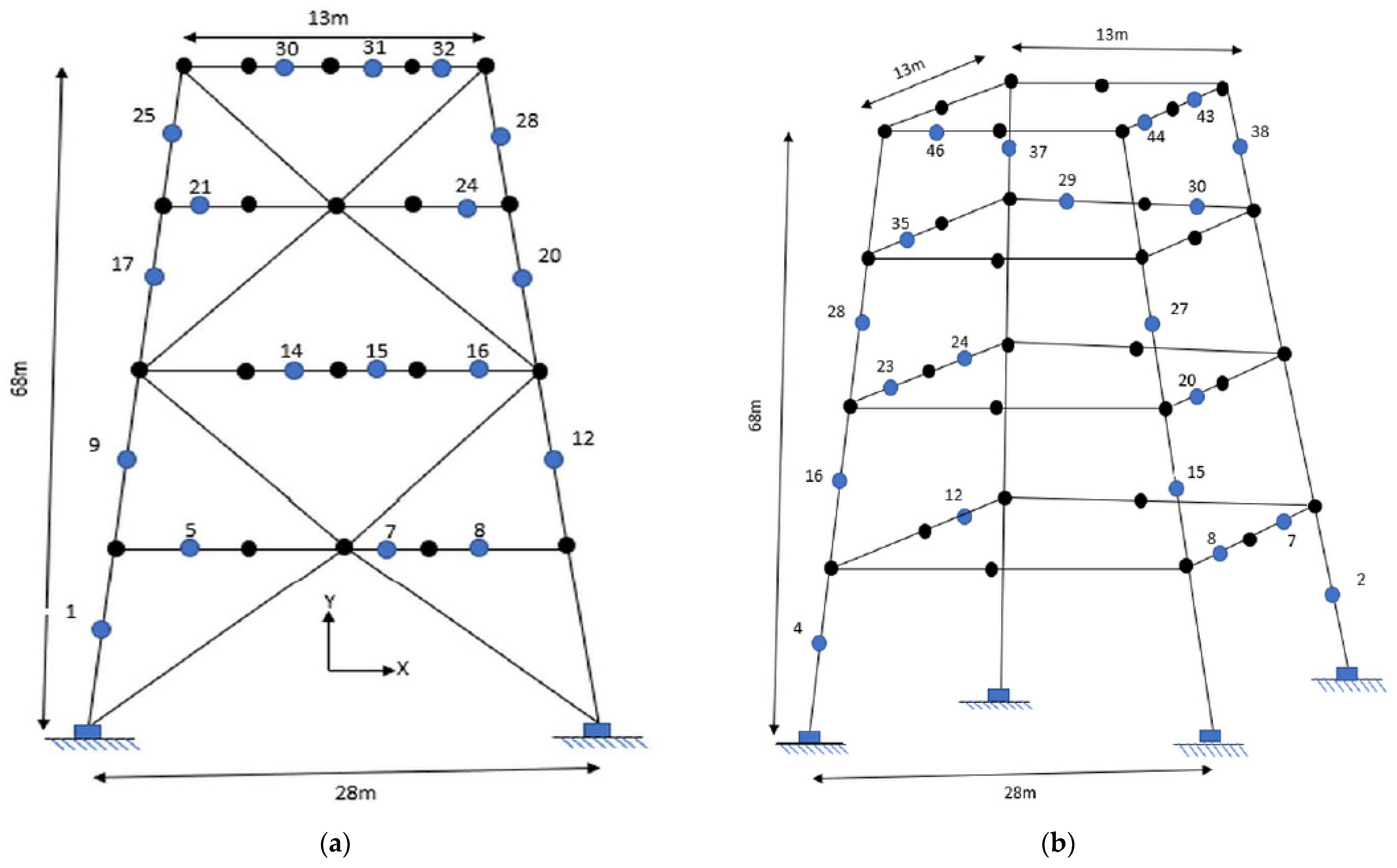
The strain energy density is close to the same strain energy density of the whole structure assigned as a target element, and it can generally be used to find the behavior of the structure. According to the circumscription of the use of strain gauges, the number of gauges in the 2D frame and 3D frames were limited to 18 and 20 units, respectively. Moreover, by using trial and error as a fundamental method for solving the problem, the strain gauges were placed in various positions along the length of the elements, where these distances were 3/4, 1/2, and 1/4. The positions of the strain gauges in the 2D and 3D frames are depicted in Figure 2.
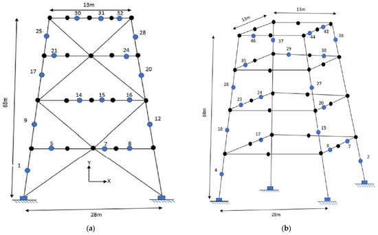
Figure 2.
Installing the strain gauges in (a) two-dimensional and (b) three-dimensional frames.
5. Damage Detection of Offshore Structures Using the Proposed Formulation
5.1. Two-Dimensional Frame Analysis
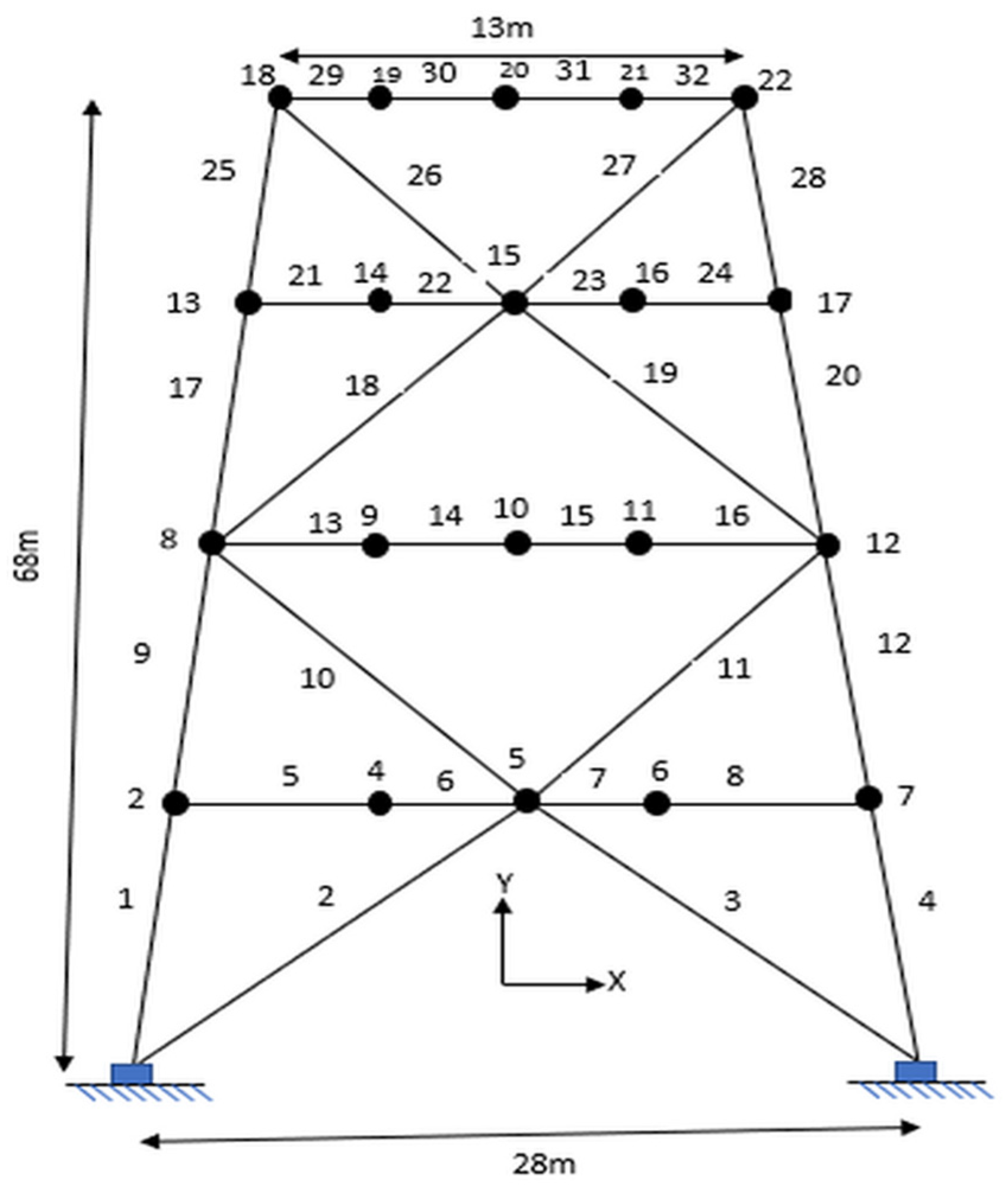
Based on Figure 3, a one-bay four-story frame was modeled to investigate the sufficiency of the proposed method in order to complete the model and identification of the structural damages. All 32 elements of the frame were constructed of steel material. The specification of the steel structure, including the elasticity modulus, density, circular cross-section with a thickness of 2 cm, and moment of inertia were 2.1 GPa, 7850 kg/m3, 307 cm2, and 91,430 kg/m2 respectively. During the simulation of a damaged two-dimensional frame structure, measurements were taken at specific locations. These locations include elements at positions 32, 31, 30, 28, 25, 24, 21, 20, 17, 16, 15, 14, 12, 9, 8, 7, 5, and 1.
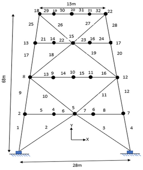
Figure 3.
Two-dimensional frame structure equipped with gauges.
The unknown parameters in the two-dimensional frame were flexural rigidity (EI) and axial rigidity (EA), where E and A are used to define the elasticity modulus and cross-section of the element, respectively. The structural response of the two-dimensional frame is influenced by both the flexural and axial behavior, by which the rigidities should be allocated to update the model.
However, the excitation of a structure in axial mode differs from reality. The measurable mode shapes are often low mode shapes, which are dominated by flexural behavior. The axial rigidity as an unknown parameter has a minimum contribution rate on the sensitivity equations, which can lead to obtaining incompatible sensitivity equations and a lack of convergence. Hence, this article places significant emphasis on the consideration of flexural rigidity.
The geometry of the frame was entered into the numerical modeling and the damage was modeled. To estimate and investigate the effectiveness of the parameters, the location and severity of several instances of damage were classified, as shown in Table 1.

Table 1.
Percentage of stiffness reduction of elements for the considered damage scenarios(2D).
For instance, the damage for case 3 was modified by three modes, where an increasing trend in element number from 22 to 31 correlated with downward and upward percentage changes in damage of approximately 10% and 20%, respectively.
Measurement errors are inevitable, where this issue is due to the preparation process of the experimental and real data; determining the damage using Wang’s method [37] and the proposed method was influenced by measurement errors. In this study, we assumed the measurement spread between the lowest and highest measured values. To resemble the measurement errors, some errors with uniform distribution were added to the correct information. To correctly simulate the measured data, one percentage of error was added to strain data with a uniform distribution.
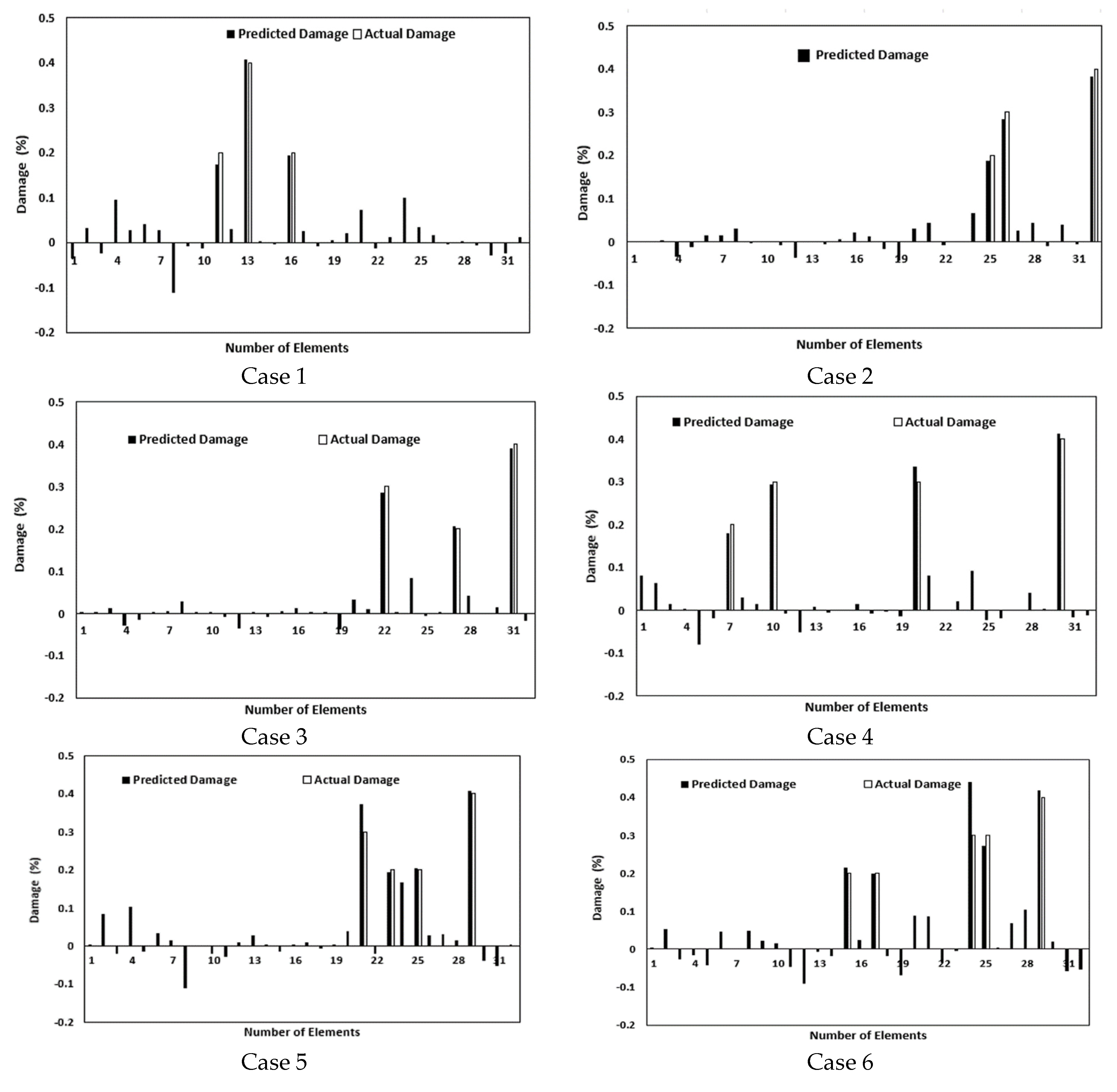
Monte Carlo simulation (MCS) is the most robust and accurate method for estimating the probability of failure [39]. MCS [40] is a statistical method that uses random variables with a probability distribution to simulate measurement errors for unknown inputs in a problem. The damage detection algorithm repeatedly uses a set of data errors that are randomly simulated, and similar conditions are applied in the damage recognition process based on the absolute difference between the methods. Numerical simulations were performed using 50 observations, and the average of all results was used as the predicted damage for each damage scenario. The results of the parameter estimation, including the predicted and actual damage ratio of the 2D frame model in six cases, are displayed in Figure 4 and Figure 5.

Figure 4.
Predicted and actual damage ratio of the 2D frame model using the present method.
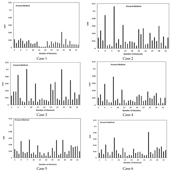
Figure 5.
The coefficient of variation of the predicted damage ratio for the 2D frame model using the current method.
Figure 4 illustrates that the proposed method was accurate in diagnosing the location and severity of the damage while the Wang method [37] did not have the ability to recognize the damage. The given information and the input data were mostly the same for both methods. Consequently, the sensitivity equation was accurate and reliable, and it improved the results of the model updating.
Scattering of the obtained damage detection results using 50 Monte Carlo simulations [40] around the average value could be measured by using a standard statistical measurement known as the coefficient of variation (COV) or relative standard deviation (RSD), which gives the ratio of the standard deviation to the average value. The COV index is used for robustness evaluation against measurement errors, and a low level of the COV denotes the power of the method. In more detail, a higher COV value indicates that small changes in the monitored variable can have a larger impact on the structure, making it more sensitive to variability. In terms of health monitoring, higher COV values can affect reliability and safety, introducing uncertainty and variability that may impact the overall performance. When assessing risks and making decisions related to health monitoring, higher COV values suggest a higher level of risk and uncertainty, calling for additional measures to mitigate potential failures or accommodate variability in the design. Therefore, COV values in health monitoring provide important insights into the variability and its implications for reliability, safety, and risk assessment.
The COV does not have a limited number or an upper bound. The COV is calculated as the ratio of the standard deviation to the mean of a variable, expressed as a percentage. Since both the standard deviation and mean can take any positive value, the COV can theoretically range from 0% to positive infinity. However, it is important to note that the COV is not a suitable measure for variables with a mean close to zero or approaching zero, as it can lead to undefined or misleading results. The coefficients of variation of the predicted damage are shown in Figure 5.
The COVs indicated less variability in the results of the evaluated parameters in the proposed method. Certain metrics are employed to quantitatively compare the accuracy of the results. This accuracy can be assessed through the closeness index (CI), which measures the proximity between the actual and predicted damage vectors.
The closeness index (CI) [41] is a measure of the accuracy of the predicted damage parameters. It is calculated as the distance between the actual damage vector () and the predicted damage vector (), with dimensions of npxp, as shown in Equations (17) and (27).
The CI quantitatively evaluates how similar the predicted damage vector is to the actual damage vector. Higher values of the CI indicate greater similarity between the predicted and actual damage vectors, leading to more accurate damage detection results. Using the CI as a performance metric allows researchers to compare the effectiveness of different damage detection methods, which can result in the development of more precise and dependable techniques for structural systems. The use of the CI can also enhance the overall safety and performance of structural systems by enabling the early detection of damage, which can be repaired or reinforced before a catastrophic failure occurs, thus increasing the system’s durability and resilience.
The accuracy of the proposed method based on the results obtained is presented in Table 2. The CI index is defined in this table to determine the accuracy of the failure detection. The closer the CI value is to one, the more accurately the failure value is predicted, and the closer it is to zero, the less accurately the failure value is calculated [41] The proposed method in this study identified the damaged elements (Table 1) with high accuracy. The accuracy of the method was evaluated by calculating the proximity index; for example, in the first case, 0.64768 was obtained, indicating the accuracy of the proposed method. Additionally, this table demonstrates that the results were reliable and had low variability.
Table 2.
Closeness indexes of the estimated parameters of the 2D frame model using the present method.
The results of the CI for different damage cases are presented in Table 2 and indicate the effectiveness of the proposed method in improving the sensitivity equation.
5.2. The Assessment of the 3D Frame
Referring to Figure 6, a one-bay four-story frame was modeled to investigate the usefulness of the proposed method in order to produce the model and identify the damage. Finite element analysis was performed for a three-dimensional frame element to simulate and compare the experimental data.
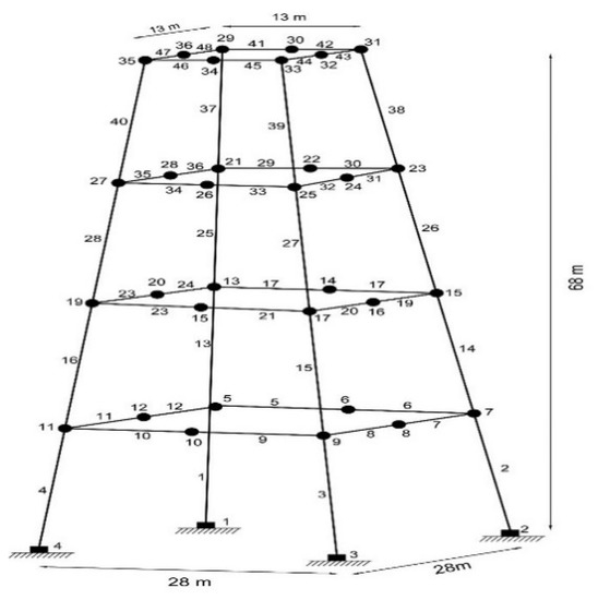
Figure 6.
Three-dimensional frame structure.
In the 3D frame, the steel element properties were as follows: elasticity modulus of 2.1 GPa, a density of 7850 kg/m3, and a moment of inertia limited to 91,430 kg/m2. Moreover, the cross-section’s element was 307 cm2. To process data of a damaged structure, measurements were made using elements 2, 4, 7, 12, 8, 15, 16, 20, 23, 24, 27, 28, 29, 30, 35, 37, 38, 43, 44, and 46.
The unknown parameters in a three-dimensional frame are the torsional rigidity GJ, flexural rigidity EI, and axial rigidity EA, where E is the elasticity modulus, G is the shear modulus, and A is the cross-section of each element. In three-dimensional mode, torsional and flexural rigidity appeared too. Several instances of damage are explained in Table 3. For instance, for damage case 2, the number of elements changed simultaneously with the damage percent. In more detail, for element number 32, when the damage rate was limited to 50 percent, and for element number 45, the damage rate remained the same.
Table 3.
Percentage of stiffness reduction of elements for considered damage scenarios(3D).
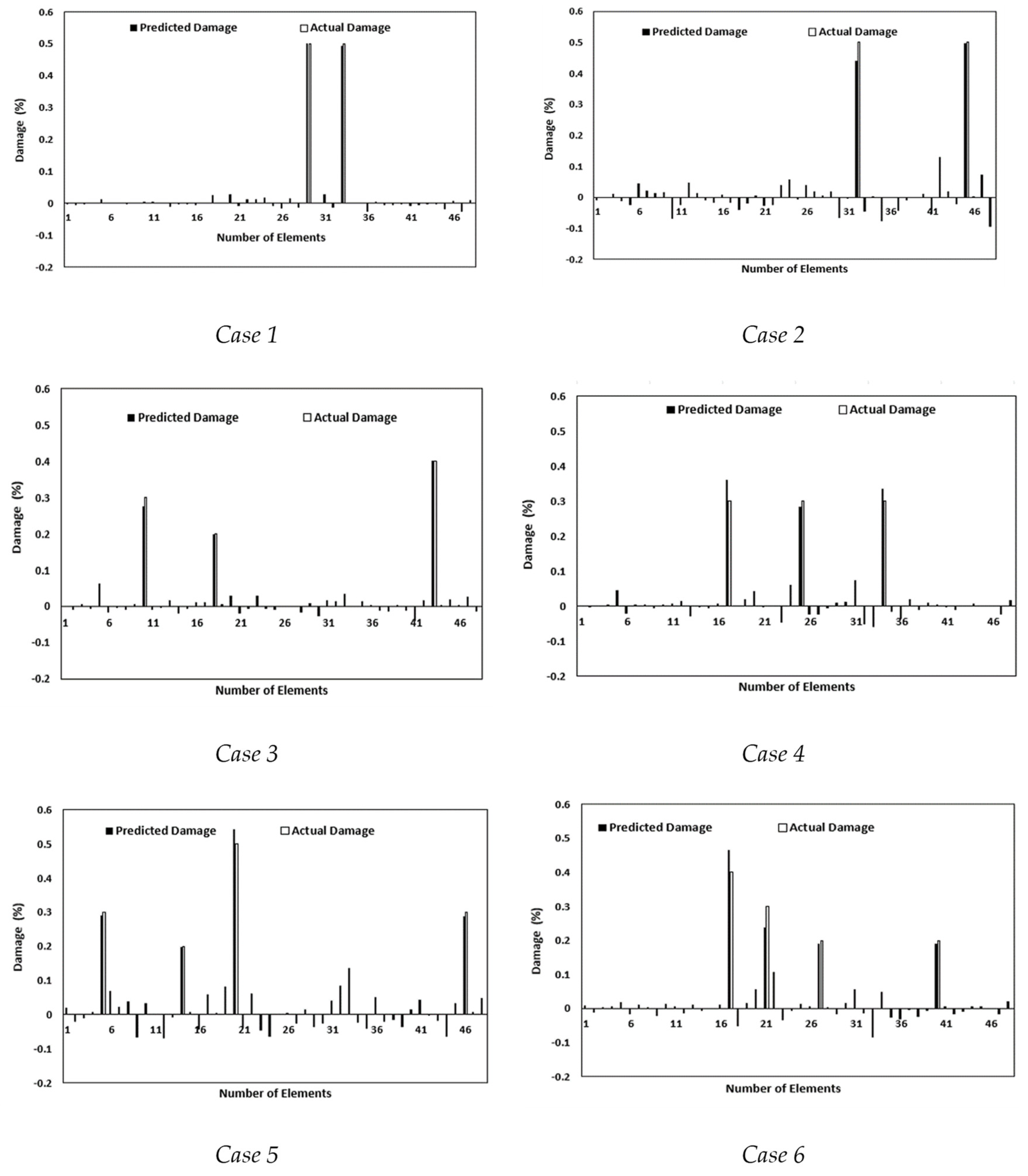
In order to check the effects of the damage location and severity to estimate the considered parameters, we updated the model results by using 50 sets of data containing modeling errors, as shown in Figure 7. A comparison between the damage prediction results using the Wang and proposed methods indicated that accurate results of parameter estimation could be achieved using the presented method, while Wang’s method was not able to recognize the damage. Results of the parameter estimation base using the CI index are shown in Table 4. The obtained CI values denoted the accuracy of the proposed method for predicting the stiffness parameters of a moment frame. The COV values for the predicted damage are shown in Figure 8.
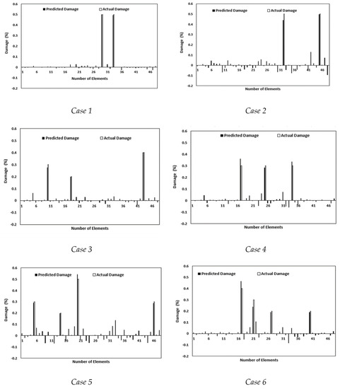
Figure 7.
Predicted and actual damage ratio of the 3D frame model using the present method.
Table 4.
Closeness index of the estimated parameters of the 3D frame model using the present method.
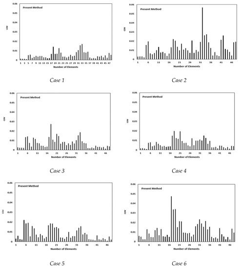
Figure 8.
The coefficient of variation of the predicted damage ratio for the 3D frame model using the current method.
6. Conclusions
This research focused on the goals of structural health monitoring (SHM) and the limitations of Wang’s method in accurately assessing damage in two-dimensional and three-dimensional structural elements, particularly in offshore structures. This study reviewed Wang’s method and proposed a new method to enhance its accuracy and applicability for 2D and 3D structural elements.
In this study, six damage cases were considered for assessing and achieving the CI and COV indexes, and by using the proposed equation, the failure rates in 2D and 3D structural elements were calculated with appropriate accuracies. For example, a COV value of 0.04 suggests that the standard deviation is only 4% of the mean value, indicating that the data points are relatively close to the mean and exhibit limited variability. This level of consistency can be advantageous in applications where precision, accuracy, and reliability are critical, such as in high-precision manufacturing, quality control processes, or safety-critical systems. This method can be used to improve structures with axial and bending behavior. Due to the high sensitivity of the strain to failure and the high accuracy of the sensitivity equations, an enhanced SHM method for accurate damage detection in 2D and 3D structures that accommodates model updates and measurement errors enhances the reliability and effectiveness of structural health monitoring systems.
The following could be the focus of potential future studies: Due to the importance of seismic loads for offshore structures, the impact of the ground motion record [42,43] on the SHM of offshore structures using the proposed damage detection method can be investigated in future works.
Combining the probabilistic risk assessment methodology introduced in [44] and the proposed damage detection formulation for assessing the lifecycle of offshore structures.
A comparison of the proposed method with other well-known damage detection techniques, such as the finite element method, to evaluate the performance and accuracy of the method in different structures.
An evaluation of structural damage through the soil–structure interaction by considering the seismic analysis results of soil deposits, which can obtain a better understanding of the behavior of the soil–structure system and design structures that can withstand the effects of earthquakes [45].
An extension of the proposed method to more complex structures, such as bridges [46] and post-tensioned joints [47,48], to validate the method’s adaptability to a wider range of structures. The damage assessment of joints in the frame structure [49] can be a useful way to produce better designs based on performance.
An integration of the proposed method with other structural health monitoring techniques, such as strain and load monitoring, to provide a comprehensive view of a structure’s behavior and health.
An extension of the proposed method to include the analysis of non-linear structures, such as those with large deformations and material non-linearities, to evaluate its applicability to a wider range of structures.
Author Contributions
Conceptualization, M.Z.K. and A.T.; methodology, M.Z.K. and S.Y.; software, M.Z.K.; validation, M.Z.K., A.T. and S.Y.; formal analysis, A.T.; investigation, S.Y.; resources, M.Z.K.; data curation, S.Y.; writing—original draft preparation, M.Z.K.; writing—review and editing, A.T.; visualization, S.Y.; supervision, A.T.; project administration, A.T. All authors have read and agreed to the published version of the manuscript.
Funding
This research received no external funding.
Data Availability Statement
Not Applicable.
Conflicts of Interest
The authors declare no conflict of interest.
Nomenclature
| A | Structure stiffness joint matrix |
| Ae | Non-zero eigenvector stiffness matrix |
| B | Strain–displacement matrix |
| d | Damage mode index |
| I | Healthy mode index |
| K | Structure stiffness matrix |
| M | Structure mass matrix |
| ne | Number of elements |
| P | Diagonal matrix of stiffness parameters |
| Pe | Stiffness parameters vector |
| T | Transform matrix |
| Ue | Displacement vector’s eth element |
| e | Strain of eth element |
| I | ith mode shape |
| I | ith natural frequency |
References
- Zarrin, M.; Asgarian, B.; Abyani, M. Probabilistic seismic collapse analysis of jacket offshore platforms. J. Offshore Mech. Arct. Eng. 2018, 140, 031601. [Google Scholar] [CrossRef]
- Khedmatgozar Dolati, S.S.; Caluk, N.; Mehrabi, A.; Khedmatgozar Dolati, S.S. Non-Destructive Testing Applications for Steel Bridges. Appl. Sci. 2021, 11, 9757. [Google Scholar] [CrossRef]
- Anders, A. Vibrational Based Inspection of Civil Engineering Structures. Ph.D. Thesis, Aalborg University, Aalborg, Denmark, 1993. [Google Scholar]
- Vahedi, M.; Khoshnoudian, F.; Hsu, T.Y.; Partovi Mehr, N. Transfer function-based Bayesian damage detection under seismic excitation. Struct. Des. Tall Spec. Build. 2019, 28, e1619. [Google Scholar] [CrossRef]
- Lee, J.S.; Choi, I.Y.; Cho, H.N. Modeling and detection of damage using smeared crack model. Eng. Struct. 2004, 26, 267–278. [Google Scholar] [CrossRef]
- Modak, S.V. Model updating using uncorrelated modes. J. Sound Vib. 2014, 333, 2297–2322. [Google Scholar] [CrossRef]
- Lim, T.W. Submatrix approach to stiffness matrix correction using modal test data. AIAA J. 1990, 28, 1123–1130. [Google Scholar] [CrossRef]
- Maeck, J.; Wahab, M.A.; Peeters, B.; De Roeck, G.; De Visscher, J.; De Wilde, W.P.; Ndambi, J.-M.; Vantomme, J. Damage identification in reinforced concrete structures by dynamic stiffness determination. Eng. Struct. 2000, 22, 1339–1349. [Google Scholar] [CrossRef]
- Carvalho, J.; Biswa, N.D.; Abhijit, G.; Maitreya, L. A direct method for model updating with incomplete measured data and without spurious modes. Mech. Syst. Signal Process. 2007, 21, 2715–2731. [Google Scholar] [CrossRef]
- Mottershead, J.E.; Link, M.; Friswell, M.I. The sensitivity method in finite element model updating: A tutorial. Mech. Syst. Signal Process. 2011, 25, 2275–2296. [Google Scholar] [CrossRef]
- Charbel, F.; Hemez, F.M. Updating finite element dynamic models using an element-by-element sensitivity methodology. AIAA J. 1993, 31, 1702–1711. [Google Scholar] [CrossRef]
- Brownjohn, J.M.W.; Pin-Qi, X.; Hong, H.; Yong, X. Civil structure condition assessment by FE model updating: Methodology and case studies. Finite Elem. Anal. Des. 1995, 37, 761–775. [Google Scholar] [CrossRef]
- Lin, R.M.; Lim, M.K.; Du, H. Improved inverse eigensensitivity method for structural analytical model updating. J. Vib. Acoust. 1995, 117, 192–198. [Google Scholar] [CrossRef]
- Gerist, S.; Maheri, M.R. Structural damage detection using imperialist competitive algorithm and damage function. Appl. Soft Comput. 2019, 77, 1–23. [Google Scholar] [CrossRef]
- Wang, L.; Lu, Z.R. Sensitivity-free damage identification based on incomplete modal data, sparse regularization and alternating minimization approach. Mech. Syst. Signal Process. 2019, 120, 43–68. [Google Scholar] [CrossRef]
- Wnag, X.; Lian, C.; Zheng, C.; Fen, L. Sensitivity analysis and dynamic modification of modal parameter in mechanical transmission system. J. Mar. Sci. Appl. 2005, 4, 53–58. [Google Scholar] [CrossRef]
- Kim, J.T.; Stubbs, N. Damage detection in offshore jacket structures from limited modal information. Int. J. Offshore Polar Eng. 1995, 5, 58–66. [Google Scholar]
- Ren, W.X.; De Roeck, G. Structural damage identification using modal data. I: Simulation verification. J. Struct. Eng. 2002, 128, 87–95. [Google Scholar] [CrossRef]
- Li, H.; Junrong, W.; Hu, S.-L.H. Using incomplete modal data for damage detection in offshore jacket structures. Ocean Eng. 2008, 35, 1793–1799. [Google Scholar] [CrossRef]
- Shahsavari, V.; Chouinard, L.; Bastien, J. Wavelet-based analysis of mode shapes for statistical detection and localization of damage in beams using likelihood ratio test. Eng. Struct. 2017, 132, 494–507. [Google Scholar] [CrossRef]
- Wang, J.; Wang, C.; Zhao, J. Frequency response function-based model updating using Kriging model. Mech. Syst. Signal Process. 2017, 87, 218–228. [Google Scholar] [CrossRef]
- Umar, S.; Bakhary, N.; Abidin, A.R.Z. Response surface methodology for damage detection using frequency and mode shape. Measurement 2018, 115, 258–268. [Google Scholar] [CrossRef]
- Hariri-Ardebili, M.A.; Mahdavi, G.; Abdollahi, A.; Amini, A. An rf-pce hybrid surrogate model for sensitivity analysis of dams. Water 2021, 13, 302. [Google Scholar] [CrossRef]
- Dahak, M.; Touat, N.; Benseddiq, N. On the classification of normalized natural frequencies for damage detection in cantilever beam. J. Sound Vib. 2017, 402, 70–84. [Google Scholar] [CrossRef]
- Khatir, S.; Dekemele, K.; Loccufier, M.; Khatir, T.; Wahab, M.A. Crack identification method in beam-like structures using changes in experimentally measured frequencies and Particle Swarm Optimization. Comptes Rendus Mécanique 2018, 346, 110–120. [Google Scholar] [CrossRef]
- Park, H.S.; Kim, J.; Oh, B.K. Model updating method for damage detection of building structures under ambient excitation using modal participation ratio. Measurement 2019, 133, 251–261. [Google Scholar] [CrossRef]
- Tiachacht, S.; Bouazzouni, A.; Khatir, S.; Wahab, M.A.; Behtani, A.; Capozucca, R. Damage assessment in structures using combination of a modified Cornwell indicator and genetic algorithm. Eng. Struct. 2018, 177, 421–430. [Google Scholar] [CrossRef]
- Zenzen, R.; Belaidi, I.; Khatir, S.; Wahab, M.A. A damage identification technique for beam-like and truss structures based on FRF and Bat Algorithm. Comptes Rendus Mécanique 2018, 346, 1253–1266. [Google Scholar] [CrossRef]
- Pérez, M.A.; Serra-López, R.A. Frequency domain-based correlation approach for structural assessment and damage identification. Mech. Syst. Signal Process. 2019, 119, 432–456. [Google Scholar] [CrossRef]
- Khatir, S.; Wahab, M.A.; Boutchicha, D.; Khatir, T. Structural health monitoring using modal strain energy damage indicator coupled with teaching-learning-based optimization algorithm and isogoemetric analysis. J. Sound Vib. 2019, 448, 230–246. [Google Scholar] [CrossRef]
- Abasi, A.; Harsij, V.; Soraghi, A. Damage detection of 3D structures using nearest neighbor search method. Earthq. Eng. Eng. Vib. 2021, 20, 705–725. [Google Scholar] [CrossRef]
- Chen, W.; Zheo, W.; Yang, H.; Chen, X. Damage detection based on optimized incomplete mode shape and frequency. Acta Mech. Solida Sin. 2015, 28, 74–82. [Google Scholar] [CrossRef]
- Iannelli, P.; Angeletti, F.; Gasbarri, P.; Panella, M.; Rosato, A. Deep learning-based Structural Health Monitoring for damage detection on a large space antenna. Acta Astronaut. 2022, 193, 635–643. [Google Scholar] [CrossRef]
- Wang, Q.; Wu, Z. Structural system reliability analysis based on improved explicit connectivity BNs. KSCE J. Civ. Eng. 2018, 22, 916–927. [Google Scholar] [CrossRef]
- Chen, H.P.; Maung, T.S. Regularised finite element model updating using measured incomplete modal data. J. Sound Vib. 2014, 333, 5566–5582. [Google Scholar] [CrossRef]
- Nelson, R.B. Simplified calculation of eigenvector derivatives. AIAA J. 1976, 14, 1201–1205. [Google Scholar] [CrossRef]
- Wang, B.P. Improved approximate methods for computing eigenvector derivatives in structural dynamics. AIAA J. 1991, 29, 1018–1020. [Google Scholar] [CrossRef]
- Sanayei, M.; Saletnik, M.J. Parameter estimation of structures from static strain measurements. I: Formulation. J. Struct. Eng. 1996, 122, 555–562. [Google Scholar] [CrossRef]
- Abdollahi, A.; Moghaddam, M.A.; Monfared, S.A.H.; Rashki, M.; Li, Y. A refined subset simulation for the reliability analysis using the subset control variate. Struct. Saf. 2020, 87, 102002. [Google Scholar] [CrossRef]
- Yuen, K.V.; James, L.B.; Siu, K.A. Structural damage detection and assessment by adaptive Markov chain Monte Carlo simulation. Struct. Control Health Monit. 2004, 11, 327–347. [Google Scholar] [CrossRef]
- Esfandiari, A.; Bakhtiari-Nejad, F.; Rahai, A.; Sanayei, M. Structural model updating using frequency response function and quasi-linear sensitivity equation. J. Sound Vib. 2009, 326, 557–573. [Google Scholar] [CrossRef]
- Alkayem, N.F.; Shen, L.; Asteris, P.G.; Sokol, M.; Xin, Z.; Cao, M. A new self-adaptive quasi-oppositional stochastic fractal search for the inverse problem of structural damage assessment. Alex. Eng. J. 2022, 61, 1922–1936. [Google Scholar] [CrossRef]
- Taslimi, A.; Tehranizadeh, M. The effect of vertical near-field ground motions on the collapse risk of high-rise reinforced concrete frame-core wall structures. Adv. Struct. Eng. 2022, 25, 410–425. [Google Scholar] [CrossRef]
- Kia, M.; Amini, A.; Bayat, M.; Ziehl, P. Probabilistic seismic demand analysis of structures using reliability approaches. J. Earthq. Tsunami 2021, 15, 2150011. [Google Scholar] [CrossRef]
- Torabipour, A.; Hamidi, A. Ground Response Analysis of Cemented Alluviums Using Non-Recursive Algorithm. J. Earthq. Eng. 2020, 24, 1390–1416. [Google Scholar] [CrossRef]
- Vahdati, V.J.; Yaghoubi, S.; Torabipour, A.; Correia, J.A.F.O.; Fazeres-Ferradosa, T.; Taveira-Pinto, F. Combined solutions to reduce scour around complex foundations: An experimental study. Mar. Syst. Ocean Technol. 2020, 15, 81–93. [Google Scholar] [CrossRef]
- Shiravand, M.R.; Torabipour, A.; Mahboubi, S. Parametric study on effect of adding stiffener to post-tensioned steel connection. Int. J. Steel Struct. 2019, 19, 478–494. [Google Scholar] [CrossRef]
- Torabipour, A.; Abdollahi, A.; Yaghoubi, S. Assess the Effectiveness of SMA on Response of Steel Connection with PT Strands. KSCE J. Civ. Eng. 2019, 23, 5133–5142. [Google Scholar] [CrossRef]
- Yang, J.N.; Xia, Y.; Loh, C.H. Damage identification of bolt connections in a steel frame. J. Struct. Eng. 2014, 140, 04013064. [Google Scholar] [CrossRef]


Disclaimer/Publisher’s Note: The statements, opinions and data contained in all publications are solely those of the individual author(s) and contributor(s) and not of MDPI and/or the editor(s). MDPI and/or the editor(s) disclaim responsibility for any injury to people or property resulting from any ideas, methods, instructions or products referred to in the content. |
© 2023 by the authors. Licensee MDPI, Basel, Switzerland. This article is an open access article distributed under the terms and conditions of the Creative Commons Attribution (CC BY) license (https://creativecommons.org/licenses/by/4.0/).