
The Impact of Building Level of Detail Modelling Strategies: Insights into Building and Urban Energy Modelling


Abstract
:1. Introduction
1.1. Literature Review
1.2. Contributions
1.3. Structure
2. Materials and Methods
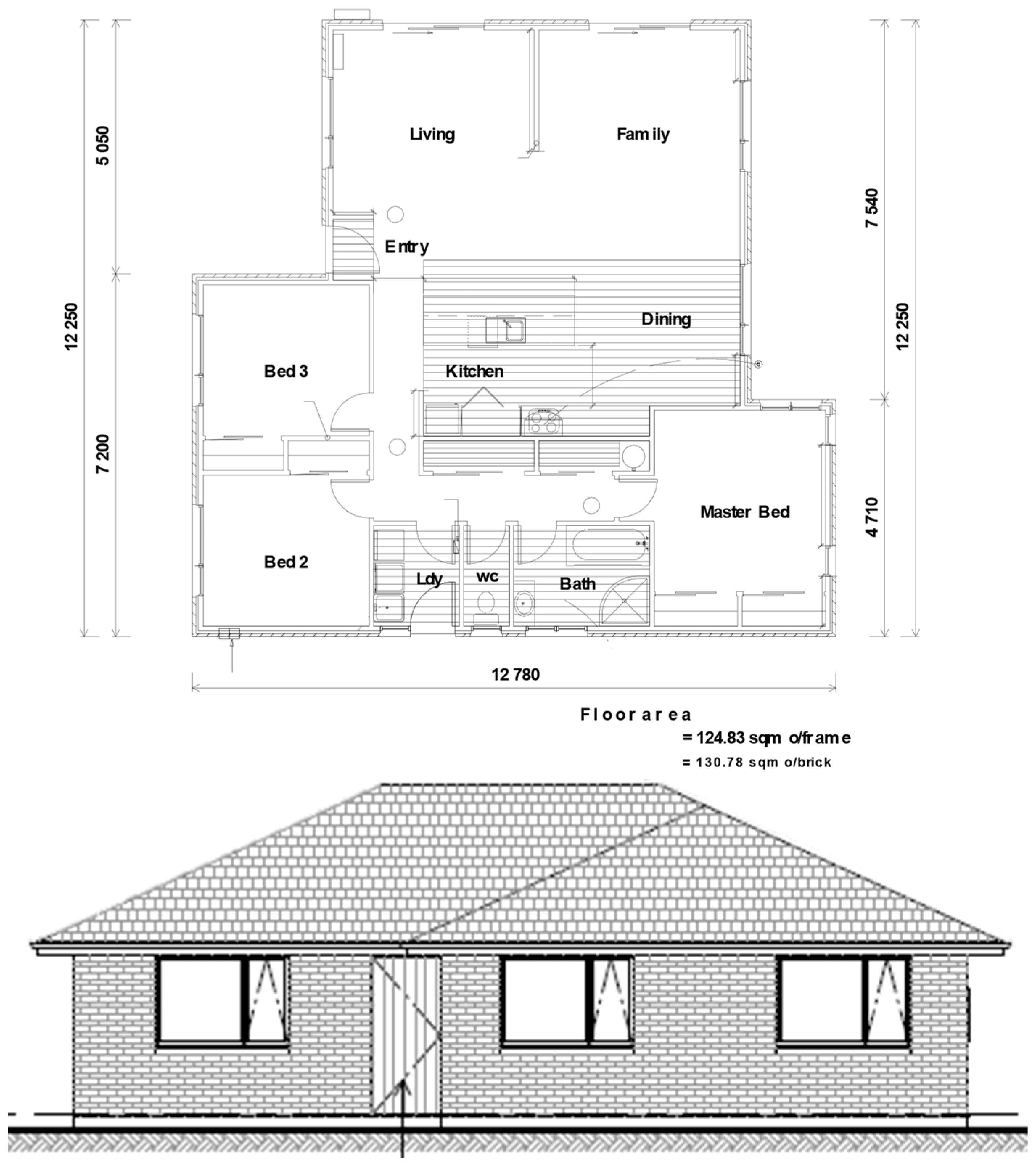
2.1. Materials
2.2. Methodology
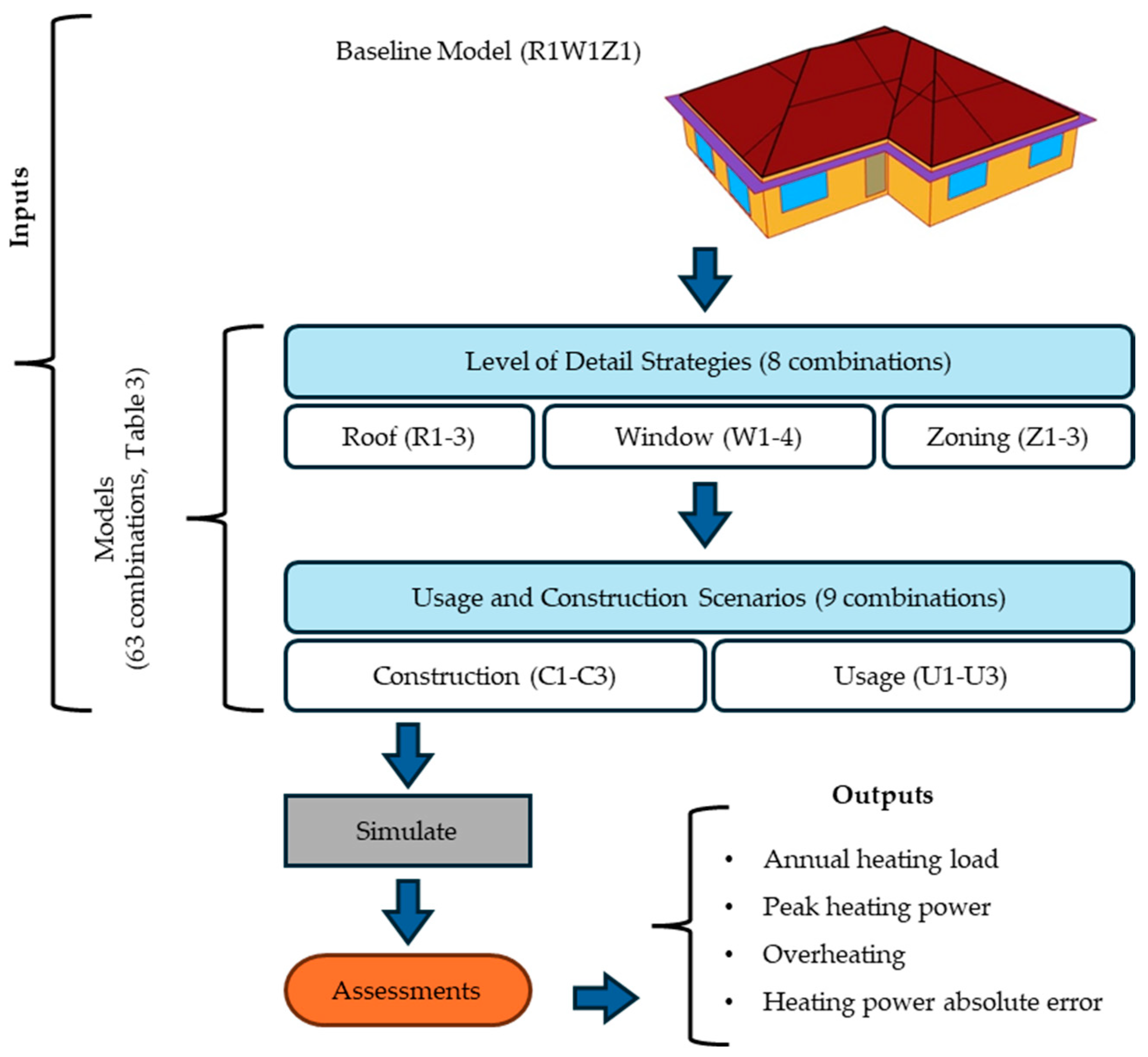
2.2.1. Level of Detail Strategies
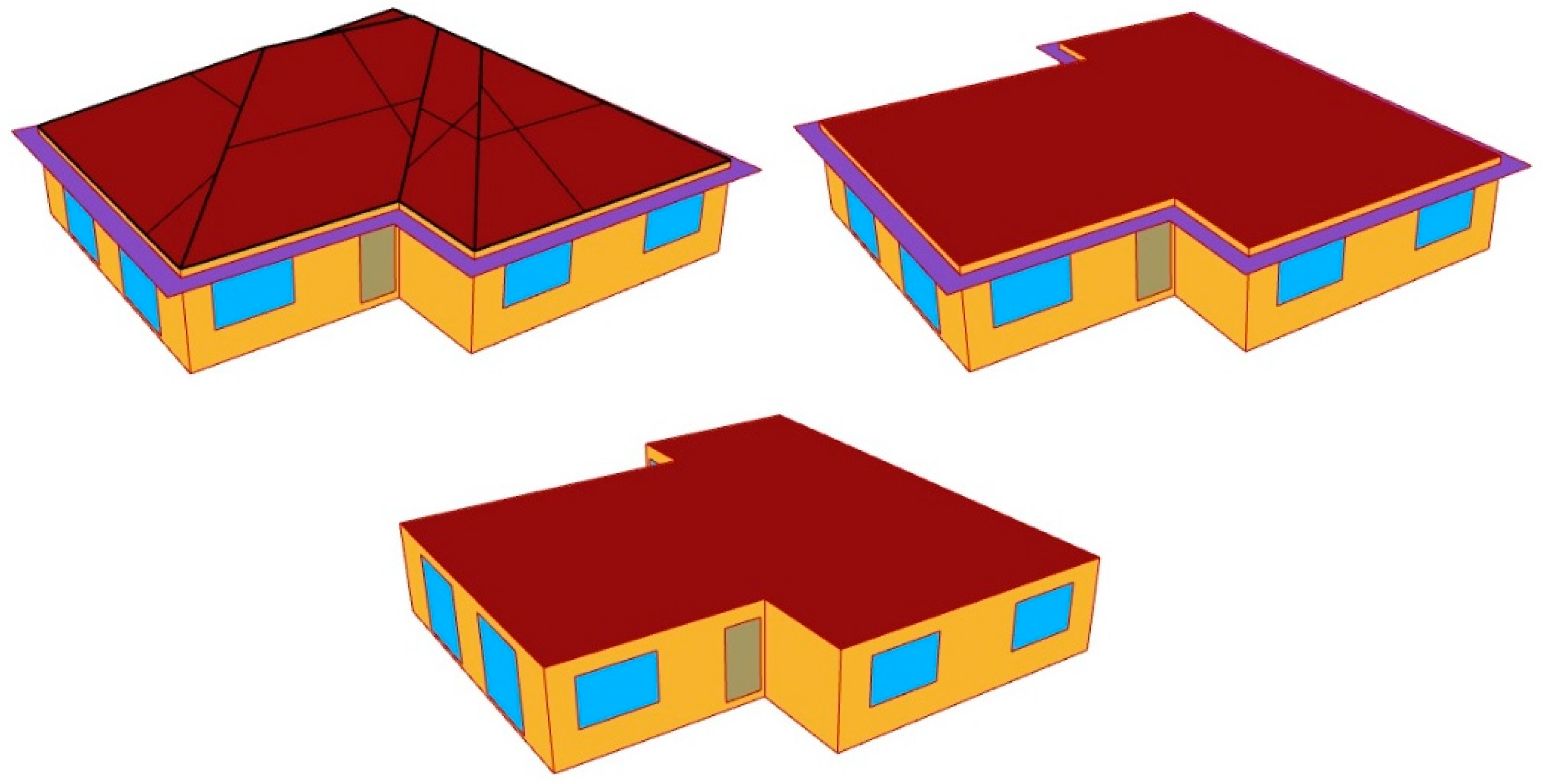
Roof LoD
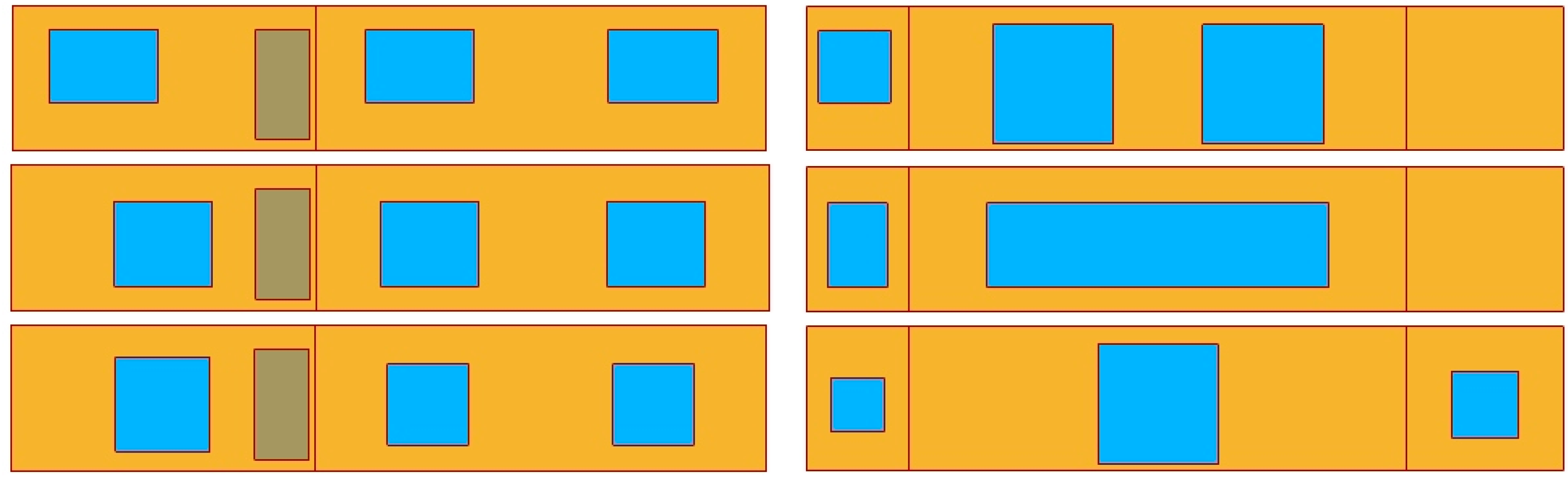
Window LoD
Zoning LoD
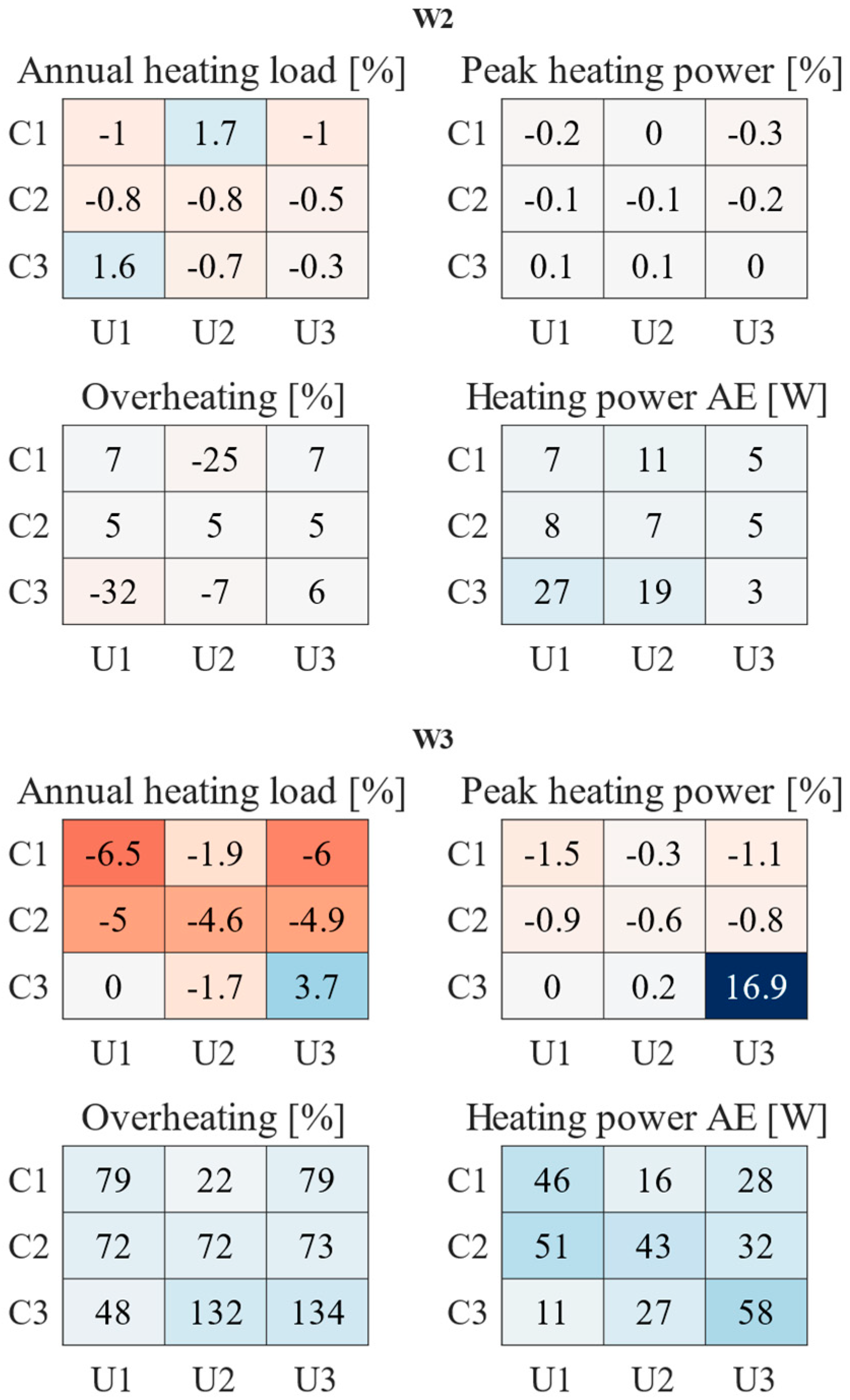
2.2.2. Construction and Usage Profiles
Construction Profiles
Usage Profiles
2.2.3. Modelling Scenarios
2.2.4. Assessments
3. Results
3.1. Roof
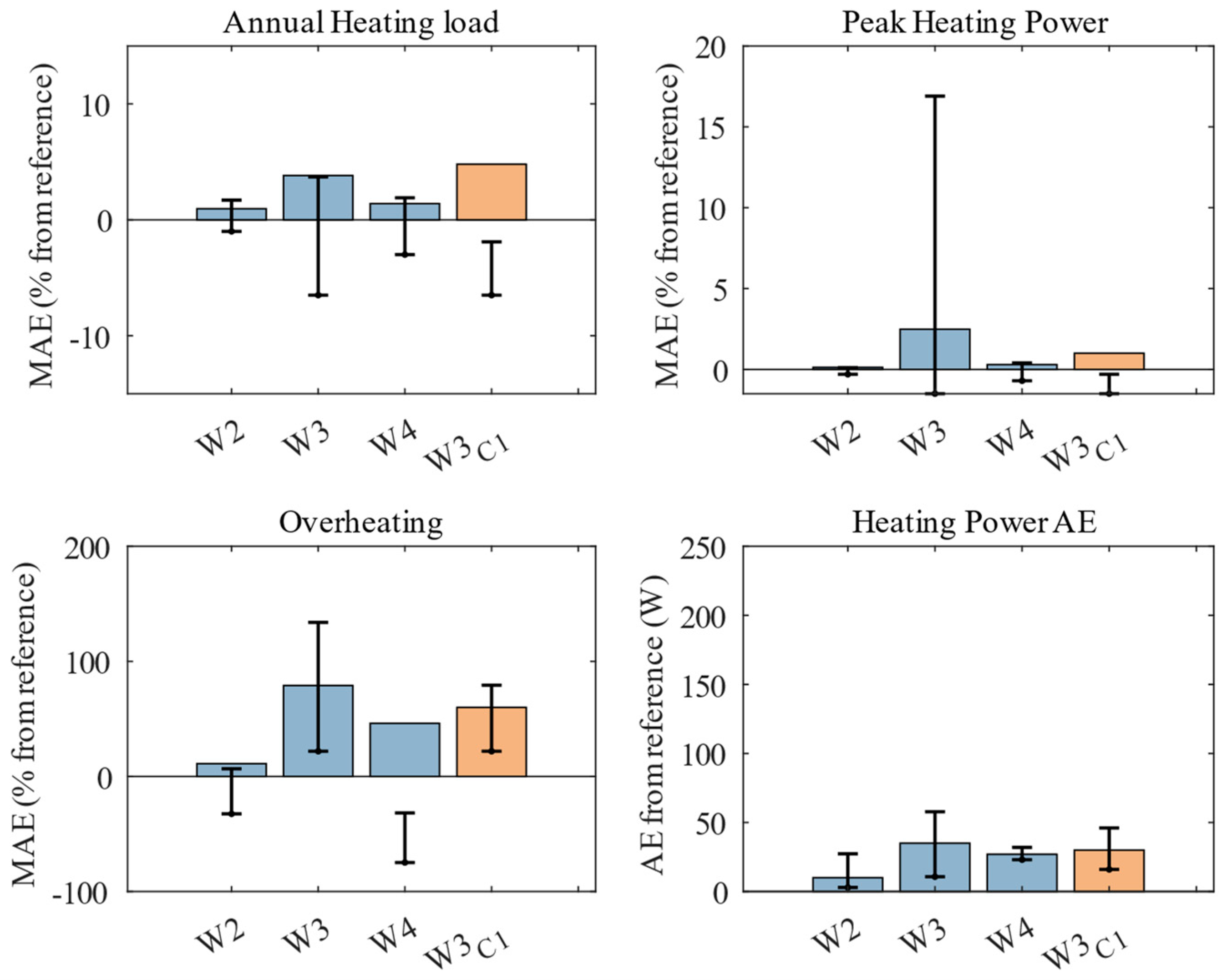
3.2. Windows
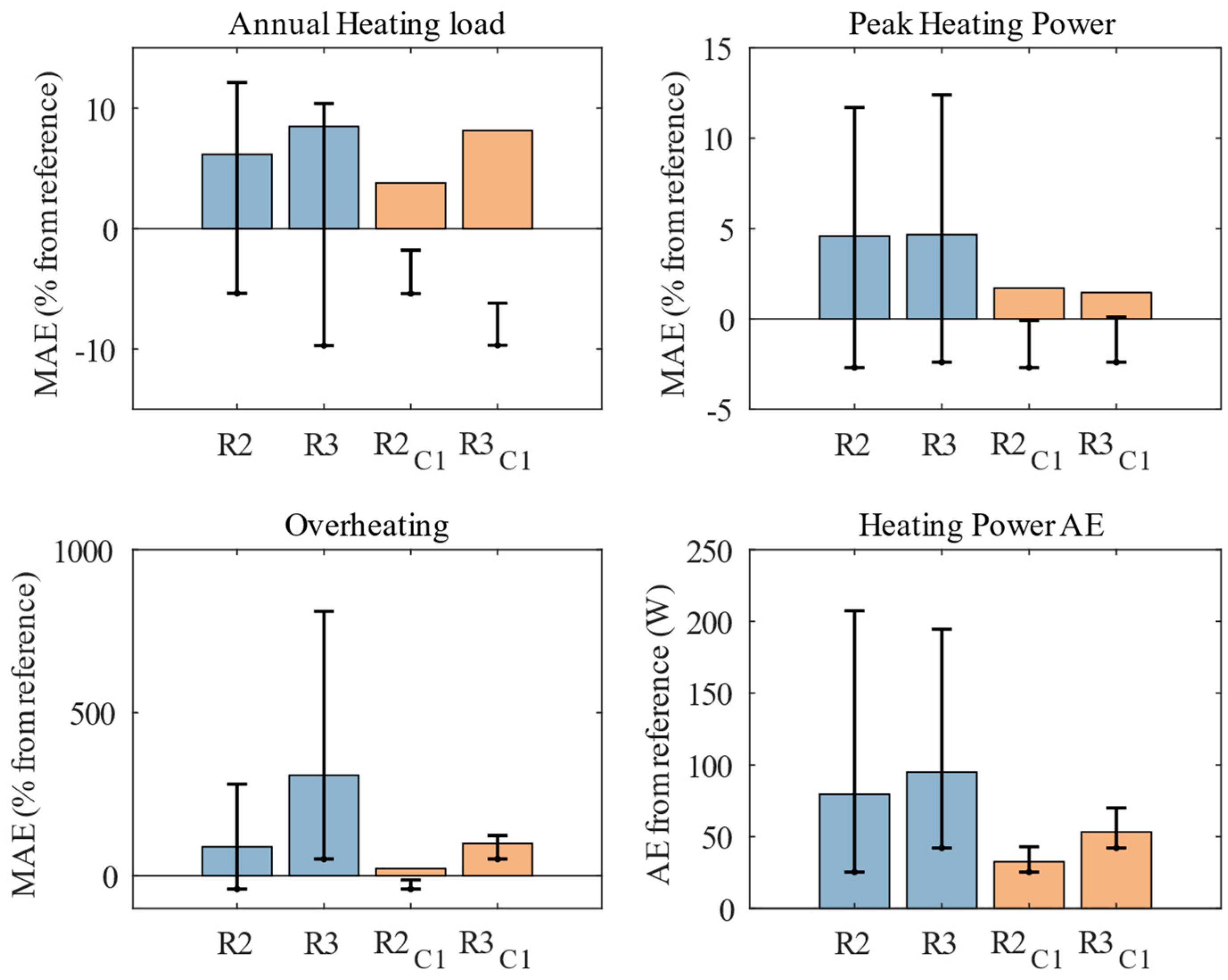
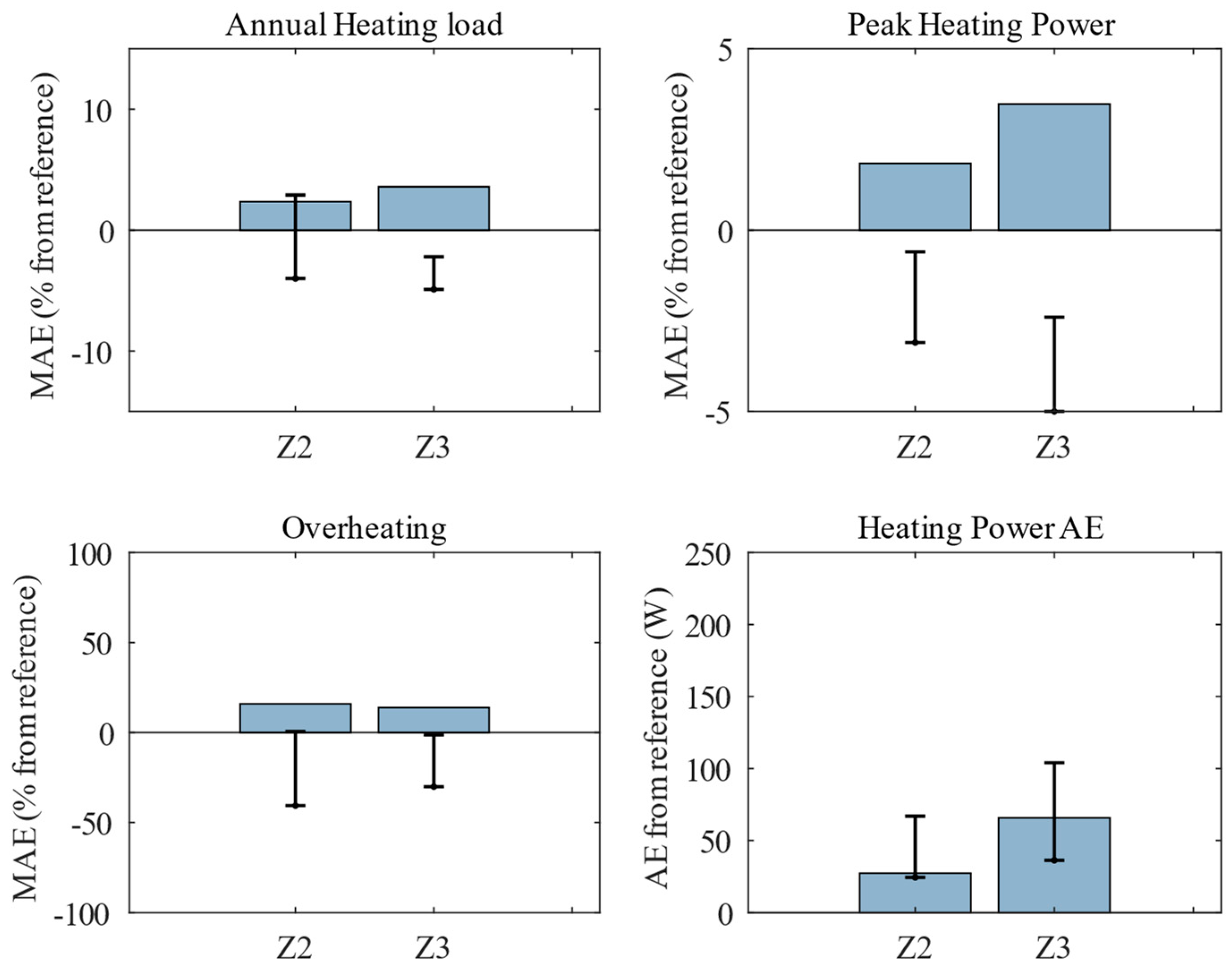
3.3. Zoning
3.4. Ranking of Error
- Zoning strategy has a considerable impact on peak demand and other time-sensitive results.
- Removing the roof air volume (R2) consistently leads to moderate error across each assessment category.
- Eaves shading (R3) and window placement (W3 and W4) both affect solar gains through windows and through the building fabric, and both introduce error in all assessment categories.
4. Discussion
4.1. Roof
4.2. Windows
4.3. Zoning
4.4. On the Accuracy of Shoebox Models
- Generally, single-zone models cannot represent variations in spatial heating behaviour; therefore, the use of single zone-models is restricted in these applications.
- Annual heating and peak heating power are significantly underestimated as the impacts of roof (R3), window (W4), and zoning (Z3) add constructively to error.
- Overheating is overestimated due to the impact of roof LoD (R3) dominating other sources of error; however, the error is moderated as the window LoD (W4) tends to underestimate overheating.
- All elements contribute towards time-series error; therefore, caution is advised when using shoe-box models where temporal accuracy is required.
4.5. Limitations
5. Conclusions
Author Contributions
Funding
Institutional Review Board Statement
Informed Consent Statement
Data Availability Statement
Conflicts of Interest
Appendix A

| Category | Level | |
|---|---|---|
| Occupant gains | Occupancy density (people/m2) | 0.031 |
| Occupants number | 4 | |
| Metabolic rate per person (W/person) | 100 | |
| Plug load gains | Equipment’s gain power density (W/m2) | 24.5 |
| Schedule Type | Days | 00:00–08:00 | 08:00–11:00 | 11:00–18:00 | 18:00–22:00 | 22:00–24:00 |
|---|---|---|---|---|---|---|
| Occupancy | Weekdays | 1 | 0.6 | 0.6 | 1 | 1 |
| Weekends and holidays | 1 | 1 | 0.5 | 0.7 | 1 | |
| Plug | All days | 0.03 | 0.23 | 0.23 | 0.27 | 0.2 |
| Surface | Layers (Outer-to-Inner) | Thickness (m) | Thermal Conductivity (W/m·k) | Specific Heat (J/kg·K) |
|---|---|---|---|---|
| External wall | Brick | 0.07 | 0.6 | 840 |
| Air gap | 0.05 | 0.0262 | 1005 | |
| Timber frame | 0.0126 | 0.14 | 1400 | |
| Wall insulation | 0.0452 | 0.04 | 840 | |
| Timber frame | 0.0126 | 0.14 | 1400 | |
| Plasterboard | 0.01 | 0.17 | 1090 | |
| Internal partition | Plasterboard | 0.01 | 0.17 | 1090 |
| Timber frame | 0.0126 | 0.14 | 1400 | |
| Cavity | 0.0012 | 0.0262 | 1005 | |
| Timber frame | 0.0126 | 0.14 | 1400 | |
| Plasterboard | 0.01 | 0.17 | 1090 | |
| Ceiling | Ceiling insulation | 0.09 | 0.04 | 840 |
| Timber frame | 0.0126 | 0.14 | 1400 | |
| Ceiling insulation | 0.0577 | 0.04 | 840 | |
| Timber frame | 0.0126 | 0.14 | 1400 | |
| Plasterboard | 0.013 | 0.17 | 1090 | |
| Roof | Corrugated iron | 0.002 | 52 | 449 |
| Floor | Ground | 0.0422 | 0.04 | 840 |
| Sandstone | 0.015 | 0.2 | 710 | |
| Concrete | 0.0226 | 1.4 | 1000 | |
| EPS foam | 0.018 | 0.03 | 1400 | |
| Concrete | 0.0226 | 1.4 | 1000 | |
| Mixed concrete (2% steel) | 0.085 | 2.5 | 880 |
| Glazing | Layers (Outer-to-Inner) | Thickness (m) | Thermal Conductivity (W/m·k) |
| Generic clear glass | 0.0422 | 0.04 | |
| air | 0.015 | 0.2 | |
| Generic glear glass | 0.0226 | 1.4 |
| Glazing | Total SHGC | R-Value (m2K/W) |
| 0.74 | 0.37 |
References
- Reinhart, C.F.; Davila, C.C. Urban building energy modeling—A review of a nascent field. Build. Environ. 2016, 97, 196–202. [Google Scholar] [CrossRef]
- Johari, F.; Peronato, G.; Sadeghian, P.; Zhao, X.; Widén, J. Urban building energy modeling: State of the art and future prospects. Renew. Sustain. Energy Rev. 2020, 128, 109902. [Google Scholar] [CrossRef]
- Pasichnyi, O.; Levihn, F.; Shahrokni, H.; Wallin, J.; Kordas, O. Data-driven strategic planning of building energy retrofitting: The case of Stockholm. J. Clean. Prod. 2019, 233, 546–560. [Google Scholar] [CrossRef]
- Cano, E.L.; Groissböck, M.; Moguerza, J.M.; Stadler, M. A strategic optimization model for energy systems planning. Energy Build. 2014, 81, 416–423. [Google Scholar] [CrossRef]
- Wang, M.; Yu, H.; Liu, Y.; Lin, J.; Zhong, X.; Tang, Y.; Guo, H.; Jing, R. Unlock city-scale energy saving and peak load shaving potential of green roofs by GIS-informed urban building energy modelling. Appl. Energy 2024, 366, 123315. [Google Scholar] [CrossRef]
- Williams, B.; Bishop, D.; Gallardo, P.; Chase, J.G. Demand Side Management in Industrial, Commercial, and Residential Sectors: A Review of Constraints and Considerations. Energies 2023, 16, 5155. [Google Scholar] [CrossRef]
- Tang, L.; Li, L.; Ying, S.; Lei, Y. A Full Level-of-Detail Specification for 3D Building Models Combining Indoor and Outdoor Scenes. ISPRS Int. J. Geo-Inf. 2018, 7, 419. [Google Scholar] [CrossRef]
- Thalfeldt, M.; Kurnitski, J.; Voll, H. Detailed and simplified window model and opening effects on optimal window size and heating need. Energy Build. 2016, 127, 242–251. [Google Scholar] [CrossRef]
- gbXML, Green Building XML (gbXML) Schema. 2023. Available online: http://www.gbxml.org (accessed on 17 March 2013).
- Leite, F.; Akcamete, A.; Akinci, B.; Atasoy, G.; Kiziltas, S. Analysis of modeling effort and impact of different levels of detail in building information models. Autom. Constr. 2011, 20, 601–609. [Google Scholar] [CrossRef]
- Battini, F.; Pernigotto, G.; Gasparella, A. District-level validation of a shoeboxing simplification algorithm to speed-up Urban Building Energy Modeling simulations. Appl. Energy 2023, 349, 121570. [Google Scholar] [CrossRef]
- Battini, F.; Pernigotto, G.; Gasparella, A. A shoeboxing algorithm for urban building energy modeling: Validation for stand-alone buildings. Sustain. Cities Soc. 2023, 89, 104305. [Google Scholar] [CrossRef]
- Dogan, T.; Reinhart, C. Shoeboxer: An algorithm for abstracted rapid multi-zone urban building energy model generation and simulation. Energy Build. 2017, 140, 140–153. [Google Scholar] [CrossRef]
- Deng, Y.; Zhou, Y.; Wang, H.; Xu, C.; Wang, W.; Zhou, T.; Liu, X.; Liang, H.; Yu, D. Simulation-based sensitivity analysis of energy performance applied to an old Beijing residential neighbourhood for retrofit strategy optimisation with climate change prediction. Energy Build. 2023, 294, 113284. [Google Scholar] [CrossRef]
- Wang, C.-K.; Tindemans, S.; Miller, C.; Agugiaro, G.; Stoter, J. Bayesian calibration at the urban scale: A case study on a large residential heating demand application in Amsterdam. J. Build. Perform. Simul. 2020, 13, 347–361. [Google Scholar] [CrossRef]
- Delgarm, N.; Sajadi, B.; Azarbad, K.; Delgarm, S. Sensitivity analysis of building energy performance: A simulation-based approach using OFAT and variance-based sensitivity analysis methods. J. Build. Eng. 2018, 15, 181–193. [Google Scholar] [CrossRef]
- Aydin, E.E.; Jakubiec, J.A. Sensitivity analysis of sustainable urban design parameters: Thermal comfort, urban heat island, energy, daylight, and ventilation in Singapore. In Proceedings of the Building Simulation and Optimization 2018 Conference, Cambridge, UK, 11–12 September 2018; pp. 11–12. [Google Scholar]
- Carlucci, S.; Causone, F.; Biandrate, S.; Ferrando, M.; Moazami, A.; Erba, S. On the impact of stochastic modeling of occupant behavior on the energy use of office buildings. Energy Build. 2021, 246, 111049. [Google Scholar] [CrossRef]
- Williams, B.; Bishop, D.; Hooper, G.; Chase, J. Driving change: Electric vehicle charging behavior and peak loading. Renew. Sustain. Energy Rev. 2024, 189, 113953. [Google Scholar] [CrossRef]
- Chen, R.; Tsay, Y.-S. An Integrated Sensitivity Analysis Method for Energy and Comfort Performance of an Office Building along the Chinese Coastline. Buildings 2021, 11, 371. [Google Scholar] [CrossRef]
- Zeferina, V.; Wood, F.R.; Edwards, R.; Tian, W. Sensitivity analysis of cooling demand applied to a large office building. Energy Build. 2021, 235, 110703. [Google Scholar] [CrossRef]
- Zhu, L.; Zhang, J.; Gao, Y.; Tian, W.; Yan, Z.; Ye, X.; Sun, Y.; Wu, C. Uncertainty and sensitivity analysis of cooling and heating loads for building energy planning. J. Build. Eng. 2022, 45, 103440. [Google Scholar] [CrossRef]
- Prataviera, E.; Vivian, J.; Lombardo, G.; Zarrella, A. Evaluation of the impact of input uncertainty on urban building energy simulations using uncertainty and sensitivity analysis. Appl. Energy 2022, 311, 118691. [Google Scholar] [CrossRef]
- Bosscha, E. Sensitivity Analysis Comparing Level of Detail and the Accuracy of Building Energy Simulations. Bachelor’s Thesis, University of Twente, Enschede, The Netherlands, 2013. [Google Scholar]
- Faure, X.; Johansson, T.; Pasichnyi, O. The Impact of Detail, Shadowing and Thermal Zoning Levels on Urban Building Energy Modelling (UBEM) on a District Scale. Energies 2022, 15, 1525. [Google Scholar] [CrossRef]
- Statistics New Zealand. Housing in Aotearoa: 2020; Statistics New Zealand: Wellington, New Zealand, 2021. Available online: https://www.stats.govt.nz/assets/Uploads/Reports/Housing-in-Aotearoa-2020/Download-data/housing-in-aotearoa-2020.pdf (accessed on 1 March 2023).
- EnergyPlus. Canterbury-Christchurch CC 937800 (NIWA). 2023. Available online: https://energyplus.net/weather-location/southwest_pacific_wmo_region_5/NZL/NZL_Canterbury-Christchurch.CC.937800_NIWA (accessed on 1 March 2023).
- Howden-Chapman, P.; Viggers, H.; Chapman, R.; O’dea, D.; Free, S.; O’sullivan, K. Warm homes: Drivers of the demand for heating in the residential sector in New Zealand. Energy Policy 2009, 37, 3387–3399. [Google Scholar] [CrossRef]
- DesignBuilder. Product Overview. Available online: https://designbuilder.co.uk/software/product-overview (accessed on 15 April 2024).
- EnergyPlus. Documentation. Available online: https://energyplus.net/documentation (accessed on 15 April 2024).
- Williams, B.; Bishop, D. Flexible Futures: The Potential for Electricity Demand Response in New Zealand. Available online: https://ssrn.com/abstract=4615974 (accessed on 12 August 2024).
- Bishop, D.; Wu, W.; Bellamy, L. A Typical Buildings Approach to Modelling Urban Energy Systems. In Proceedings of the 2023 IEEE International Smart Cities Conference (ISC2), Bucharest, Romania, 24–27 September 2023; pp. 1–5. [Google Scholar]
- Isaacs, N.; Camilleri, M.; Burrough, L.; Pollard, A.; Saville-Smith, K.; Fraser, R.; Jowett, J. Energy use in new zealand households: Final report on the household energy end-use project (heep). BRANZ Study Rep. 2010, 221, 15–21. [Google Scholar]


| Ext Walls (m2K/W) | Ceiling (m2K/W) | Floor (m2K/W) | Windows (m2K/W) | |
|---|---|---|---|---|
| C1 | 1.67 | 3.90 | 1.60 | 0.37 |
| C2 | 0.58 | 3.90 | 1.60 | 0.37 |
| C3 | 0.58 | 0.72 | 1.60 | 0.37 |
| Areas | Schedule | Setpoint | |
|---|---|---|---|
| U1 | Whole floor plan | Always on | 20 °C |
| U2 | Living area and bedrooms | Always on | 20 °C |
| U3 | Living area | 6 a.m.–10 p.m. | 20 °C |
| Bedrooms | 8 p.m.–7 a.m. | 20 °C |
| LoD \ C and U | C1U1 | C2U1 | C3U1 | C1U2 | C2U2 | C3U2 | C1U3 | C2U3 | C3U3 |
|---|---|---|---|---|---|---|---|---|---|
| R1W1Z1 | R1W1Z1 -C1U1 | R1W1Z1 -C2U1 | R1W1Z1 -C3U1 | R1W1Z1 -C1U2 | R1W1Z1 -C2U2 | R1W1Z1 -C3U2 | R1W1Z1 -C1U3 | R1W1Z1 -C2U3 | R1W1Z1 -C3U3 |
| R2W1Z1 | R2W1Z1 -C1U1 | R2W1Z1 -C2U1 | R2W1Z1 -C3U1 | R2W1Z1 -C1U2 | R2W1Z1 -C2U2 | R2W1Z1 -C3U2 | R2W1Z1 -C1U3 | R2W1Z1 -C2U3 | R2W1Z1 -C3U3 |
| R3W1Z1 | R3W1Z1 -C1U1 | R3W1Z1 -C2U1 | R3W1Z1 -C3U1 | R3W1Z1 -C1U2 | R3W1Z1 -C2U2 | R3W1Z1 -C3U2 | R3W1Z1 -C1U3 | R3W1Z1 -C2U3 | R3W1Z1 -C3U3 |
| R1W2Z1 | R1W2Z1 -C1U1 | R1W2Z1 -C2U1 | R1W2Z1 -C3U1 | R1W2Z1 -C1U2 | R1W2Z1 -C2U2 | R1W2Z1 -C3U2 | R1W2Z1 -C1U3 | R1W2Z1 -C2U3 | R1W2Z1 -C3U3 |
| R1W3Z1 | R1W3Z1 -C1U1 | R1W3Z1 -C2U1 | R1W3Z1 -C3U1 | R1W3Z1 -C1U2 | R1W3Z1 -C2U2 | R1W3Z1 -C3U2 | R1W3Z1 -C1U3 | R1W3Z1 -C2U3 | R1W3Z1 -C3U3 |
| R1W4Z1 | R1W4Z1 -C1U1 | R1W4Z1 -C2U1 | R1W4Z1 -C3U1 | R1W4Z1 -C1U2 | R1W4Z1 -C2U2 | R1W4Z1 -C3U2 | R1W4Z1 -C1U3 | R1W4Z1 -C2U3 | R1W4Z1 -C3U3 |
| R1W1Z2 | R1W1Z2 -C1U1 | R1W1Z2 -C2U1 | R1W1Z2 -C3U1 | R1W1Z2 -C1U2 | R1W1Z2 -C2U2 | R1W1Z2 -C3U2 | - | - | - |
| R1W1Z3 | R1W1Z3 -C1U1 | R1W1Z3 -C2U1 | R1W1Z3 -C3U1 | - | - | - | - | - | - |
| Annual Heating Load | Peak Heating Power | Overheating | Heating Power AE (W) | |||||
|---|---|---|---|---|---|---|---|---|
| 1 | R3-C1 | 8.1% | Z3 | 3.5% | R3-C1 | 99% | Z3 | 66 |
| 2 | W3-C1 | 4.8% | Z2 | 1.8% | W3-C1 | 60% | R3-C1 | 53 |
| 3 | R2-C1 | 3.8% | R2-C1 | 1.7% | W4 | 46% | Z2 | 43 |
| 4 | Z3 | 3.6% | R3-C1 | 1.5% | R2-C1 | 22% | R2-C1 | 33 |
| 5 | Z2 | 2.3% | W3-C1 | 1.0% | Z2 | 16% | W3-C1 | 30 |
| 6 | W4 | 1.4% | W4 | 0.3% | Z3 | 14% | W4 | 27 |
| 7 | W2 | 1.0% | W2 | 0.1% | W2 | 11% | W2 | 10 |
Disclaimer/Publisher’s Note: The statements, opinions and data contained in all publications are solely those of the individual author(s) and contributor(s) and not of MDPI and/or the editor(s). MDPI and/or the editor(s) disclaim responsibility for any injury to people or property resulting from any ideas, methods, instructions or products referred to in the content. |
© 2024 by the authors. Licensee MDPI, Basel, Switzerland. This article is an open access article distributed under the terms and conditions of the Creative Commons Attribution (CC BY) license (https://creativecommons.org/licenses/by/4.0/).
Share and Cite
Bishop, D.; Mohkam, M.; Williams, B.L.M.; Wu, W.; Bellamy, L. The Impact of Building Level of Detail Modelling Strategies: Insights into Building and Urban Energy Modelling. Eng 2024, 5, 2280-2299. https://doi.org/10.3390/eng5030118
Bishop D, Mohkam M, Williams BLM, Wu W, Bellamy L. The Impact of Building Level of Detail Modelling Strategies: Insights into Building and Urban Energy Modelling. Eng. 2024; 5(3):2280-2299. https://doi.org/10.3390/eng5030118
Chicago/Turabian StyleBishop, Daniel, Mahdi Mohkam, Baxter L. M. Williams, Wentao Wu, and Larry Bellamy. 2024. "The Impact of Building Level of Detail Modelling Strategies: Insights into Building and Urban Energy Modelling" Eng 5, no. 3: 2280-2299. https://doi.org/10.3390/eng5030118
APA StyleBishop, D., Mohkam, M., Williams, B. L. M., Wu, W., & Bellamy, L. (2024). The Impact of Building Level of Detail Modelling Strategies: Insights into Building and Urban Energy Modelling. Eng, 5(3), 2280-2299. https://doi.org/10.3390/eng5030118