Accuracy of Mathematical Models and Process Simulators for Predicting the Performance of Gas-Separation Membranes

Abstract

A membrane unit for gas separation is not available in most process simulators, and therefore it needs to be built manually. However, the developed units are based on assumptions, and the system is solved numerically. The accuracy of these models with industrial data is rarely discussed in the literature, but it is needed to confirm the reliability of process simulators. In this work, the membrane unit was developed in two different simulation software such as the commercial UniSIM^® and the freeware CAPE-OPEN to CAPE-OPEN (COCO). In UniSIM^®, the membrane module was built internally using a component splitter, spreadsheet, and adjust functions. In COCO, the membrane unit was developed by program coding with the external computational software, Scilab. The developed membrane units were assessed with field data for fuel gas conditioning. Results show that the membrane unit was easier to build in UniSIM^® but when calculating the flowrate and composition of all compounds at the permeate and retentate sides, UniSIM^® gives an error of 17.4% while COCO gives a slightly lower error of 17.1%. The high error was related to the effects of plasticization and concentration polarization, which were not taken into consideration in the mathematical model.

1. Introduction

The first commercial use for gas-separation membranes was in the 1980s for hydrogen purification [1]. The membrane applications were expanded further to cover carbon dioxide capture, air separation, and gas dehydration [2]. Compared to other gas-separation technologies, the membranes consume less energy and occupy a smaller area. They are also easy to integrate and can have a continuous life of five years [3]. Industrial membranes are made from polymers in which the gas is transported due to the difference in partial pressure. Usually, the membrane consists of a porous and a selective dense layer in which the gas dissolves and diffuses to the low-pressure side, which needs a compressor thereafter [4]. The porous layer provides mechanical support to the dense layer.

Process simulators are tools that predict unit performance in terms of mass and energy. They are also used for process optimization to improve efficiency and reduce energy consumption [5]. Honeywell^® UniSIM^® is widely employed in refineries due to its accuracy. For example, it was tested with real data from a diesel hydrotreatment unit, and the error was only 2.1% [6]. However, the software requires a valid license to run. CAPE-OPEN to CAPE-OPEN (COCO) V3.7 (2023) is another simulation software and, unlike UniSIM^® R500 (2024), it is free to use. The simulator was tested for hydrogen production, and the results were very close to the commercial software Aspen HYSYS^® V12 (2021) [7]. It should be noted that UniSIM^® and HYSYS^® share the same library packages and have alike graphical user interfaces [8].

Process simulators contain many chemical units such as distillations and reactors, but they lack a membrane unit for gas separation. This is because there is no standard design for the membrane, and the performance depends on the setup. For example, the membrane physical structure can be hollow fibers or spiral wounds, and each design has a different performance. Furthermore, some membranes have only one product (dead-end design) while others have two products (permeate and retentate). The flow direction (perpendicular or cross flow) can also affect the membrane performance.

There are many studies that use computers to evaluate membrane performance. However, the results are rarely assessed with industrial data. The majority of the papers compare their model with experimental data but at a laboratory scale [9,10]. Furthermore, most of the published work uses mathematical software rather than process simulators due to the difficulty of developing the model in process simulation software. This paper fills this research gap by building the membrane unit in process simulators and evaluating the results with industrial data. This paper also discusses the accuracy of the mathematical models and the precision of simulators in solving the system.

In this work, a membrane module was built into process simulators such as the commercial UniSIM^® and the freeware COCO for fuel gas conditioning. Untreated natural gas contains impurities that need to be removed. Fuel gas conditioning increases methane concentration and cuts down impurities for better combustion. The developed membrane units in UniSIM^® and COCO were assessed with field data of an industrial membrane made by Membrane Technology and Research Inc (MTR) [11]. The simulation was used to calculate the products’ composition and flowrate. Then, the results were compared with the industrial data reported by MTR. The objective is to test the reliability of the developed models in process simulators.

The following section discusses the membrane setup and the corresponding equations. It also demonstrates the methodology for creating the membrane unit in UniSIM^® and COCO. After that, the results of UniSIM^® and COCO were compared with the industrial data in terms of composition and flowrate. A conclusion was stated based on the calculated error.

2. Methodology

As reported by MTR, raw natural gas with a flowrate of 2.5 MMSCFD enters the membrane at a temperature of 21 °C and a pressure of 5534 kPa. The gas contains mostly methane (93.2 mol%) with impurities of carbon dioxide and heavier hydrocarbons. The membrane produced a retentate stream with a higher methane concentration of 94.3 mol% using a membrane area of 32 m². The permeate stream leaves the membrane at a pressure of 721.9 kPa. It is assumed that the membrane has a spiral-wound structure with a cross-flow configuration as shown in Figure 1. This design is widely used in industrial units for gas separation due to its cost effectiveness and fabrication easiness [12,13].

The membrane material is made from rubber (polydimethylsiloxane, PDMS) with a methane permeance of 130 gas-permeation units (GPU). Technical data reported by MTR for fuel gas conditioning are presented in

Table 1. Reported data by MTR for fuel gas conditioning using a PDMS membrane [11].

Property	Feed	Retentate (Product)	Permeate	Permeance (GPU a)
Flowrate (MMSCFD *)	2.50	2.00	0.50	–
Temperature (°C)	21.11	11.67	–	–
Pressure (kPa)	5534	4997	721.9	–
N2 (mol%)	0.49	0.51	0.76	43 b
CO2 (mol%)	0.34	0.28	0.48	244
C1 (mol%)	93.23	94.3	85.9	130
C2 (mol%)	2.60	2.43	4.13	264
C3 (mol%)	1.93	1.46	3.91	424
iC4 (mol%)	0.28	0.21	0.67	553
nC4 (mol%)	0.57	0.41	1.51	670
iC5 (mol%)	0.19	0.13	0.70	1361
nC5 (mol%)	0.19	0.14	0.76	1551
nC6 (mol%)	0.18	0.13	1.18	2210 b

* MMSCFD: million standard cubic feet per day. ^a: GPU = 3.3 × 10⁻¹⁰ kmol m⁻² s⁻¹ kPa⁻¹; ^b: estimated permeance and the membrane area as follows.

.

In this work, the following membrane setup was assumed: cross-flow design, no accumulation across the membrane, and the streams have a plug flow model with no back mixing. Mass balance is applied in which the number of moles of the feed ($n_F$) is the sum of the number of moles of permeate ($n_P$) and retentate ($n_R$):

$$x_F{n}_F=y_P{n}_P+x_R{n}_R$$

(1)

where $x_F$ is the mole fraction of component i in the feed, $y_P$ is the mole fraction in the permeate, and $x_R$ is the mole fraction in the retentate. Permeate flowrate can be calculated based on the following equation:

$$y_P{n}_P=QA\left(\overline{x{P}_F-y{P}_P}\right)$$

(2)

where Q is the permeance (kmol m⁻² h⁻¹ kPa⁻¹), A is the membrane area (m²), and $\left(\overline{x{P}_F-y{P}_P}\right)$ is the average pressure difference (kPa). For a cross-flow configuration, the pressure difference can be approximated by the logarithmic-mean difference [14]:

$$\left(\overline{x{P}_F-y{P}_P}\right)\cong {\left[x_F{x}_R\left({\displaystyle \frac{x_F+x_R}{2}}\right)\right]}^{1/3}{P}_F-y_P{P}_P$$

(3)

The streams contain 10 components, and the sum of mole fractions in each stream is unity as given by the following equation:

$${\displaystyle \sum }_{i=1}^n{x}_F=1 ; {\displaystyle \sum }_{i=1}^n{x}_R=1 ; {\displaystyle \sum }_{i=1}^n{y}_P=1$$

(4)

Numerical methods are needed to solve for Equation (3), and this will require initial values. Permeate cut $\left({\theta }_g\right)$ of each component was guessed, and it was defined by:

$${\theta }_g={\displaystyle \frac{y_P{n}_P}{x_F{n}_F}}$$

(5)

Simply, the permeate cut is how much flow is recovered at the permeate side compared to the feed. Permeate flowrate can be calculated when all cuts were guessed:

$$n_p=x_{F1}{n}_{F1}{\theta }_{g1}+x_{F2}{n}_{F2}{\theta }_{g2}+x_{F3}{n}_{F3}{\theta }_{g3}+x_{F4}{n}_{F4}{\theta }_{g4}+x_{F5}{n}_{F5}{\theta }_{g5}+\cdots$$

(6)

After that, the mole fractions in permeate can be determined by:

$$y_p={\displaystyle \frac{x_F{n}_F{\theta }_g}{n_P}}$$

(7)

The retentate flowrate can be calculated from:

$$n_R=n_F-n_p$$

(8)

Then, the mole fractions of retentate can be enumerated by:

$$x_R={\displaystyle \frac{x_F{n}_F-y_p{n}_P}{n_R}}$$

(9)

Next is to determine the permeate cut (${\theta }_c)$ by Equation (2) and from the calculated values of $x_R$ and $y_P$:

$${\theta }_c={\displaystyle \frac{QA}{x_F{n}_F}}\left\{{\left[x_F{x}_R\left({\displaystyle \frac{x_F+x_R}{2}}\right)\right]}^{{\displaystyle \frac{1}{3}}}{P}_F-y_P{P}_P\right\}$$

(10)

Here we can compare the guessed permeate cuts (${\theta }_g)$ and the calculated ones (${\theta }_c)$. Adjust functions will change guessed permeate cuts simultaneously until they are equal to calculated cuts. Since numerical methods are used, the calculated value will deviate from the true value. Therefore, an error function needs to be defined as follows:

$$\mathrm{Error} \mathrm{Function}={\displaystyle \sum }_{i=1}^n{\left({\theta }_g-{\theta }_c\right)}_i^2$$

(11)

The lower the error function, the better the results. Figure 2 summarizes the required input parameters and the calculated variables. The following sub-sections discuss the development of the membrane unit in UniSIM^® and COCO.

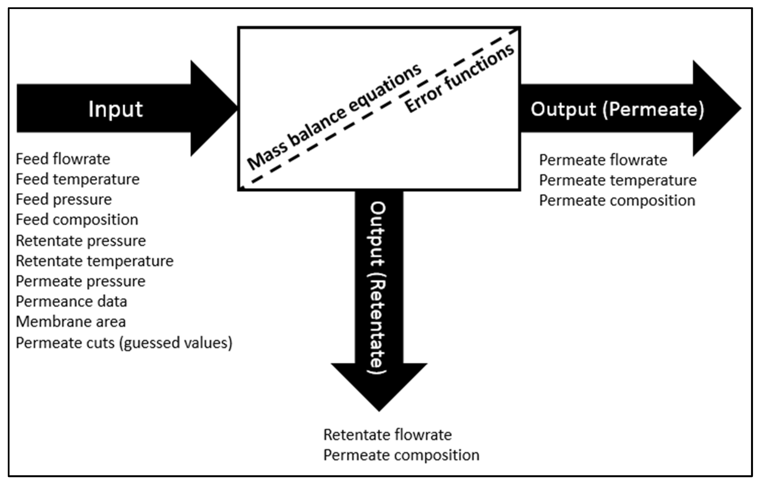
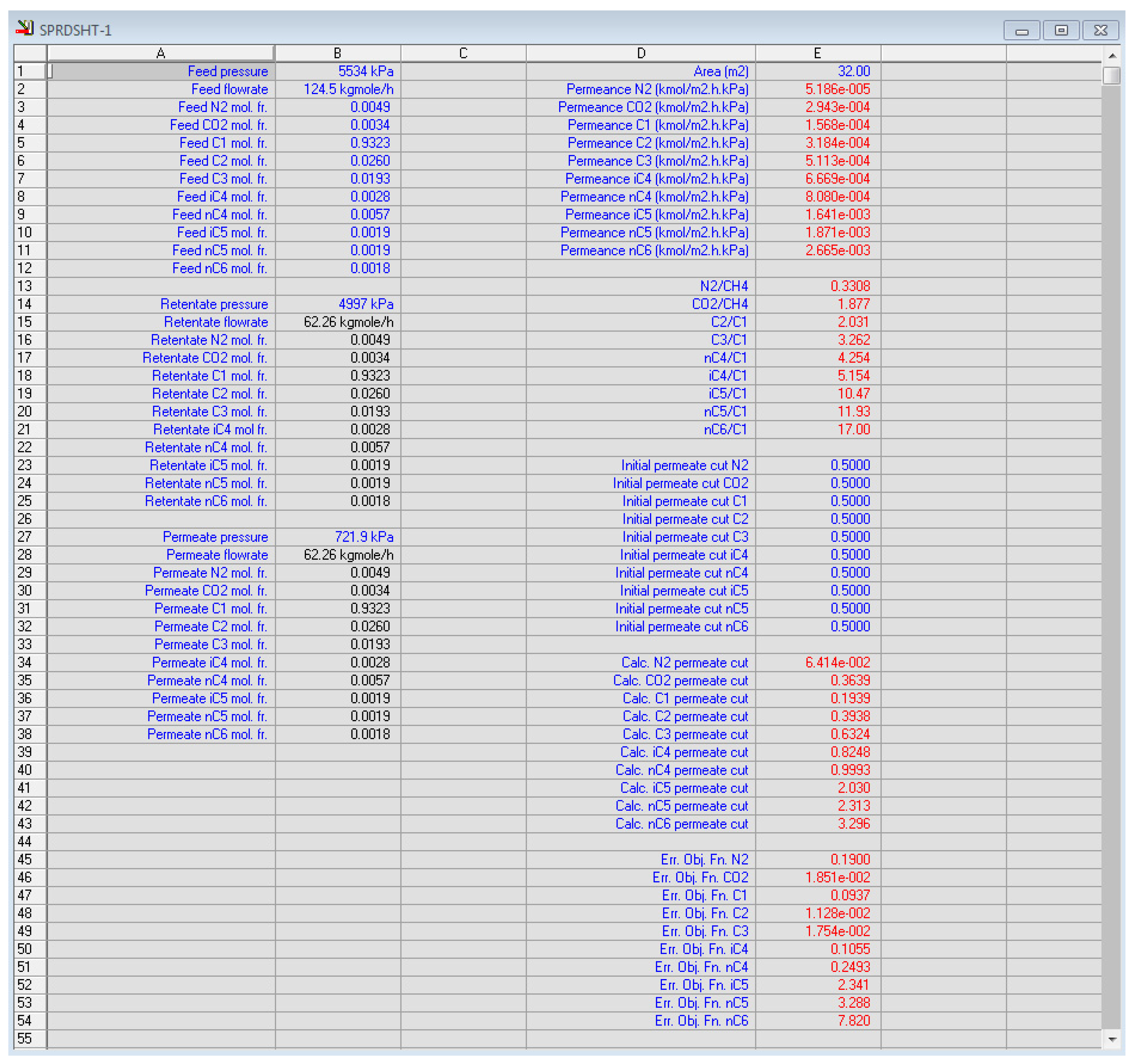
2.1. Membrane Development in UniSIM^®

Honeywell UniSIM^® was selected as the simulation software due to its accuracy and easiness. The membrane unit was built using the available tools such as component splitter, spreadsheet, and adjust functions. The component splitter is similar to a black box, but it needs permeate cuts ($\theta )$ of all the components to solve the unit. To do so, mass balance equations of the membrane (Equations (1)–(11)) are entered in the spreadsheet. The parameters in the spreadsheet such as flowrates and compositions were linked with the streams and the component splitter. Following, the adjust functions were added for each component and linked with the spreadsheet and the component splitter. The adjust functions were added as a group to solve the equations simultaneously by changing the permeate cuts (${\theta }_g$) of all components until Equation (11) is minimum. Before solving the system, the values of ${\theta }_g$ needs to be defined. As a starting point, the permeate cut of all compounds is assumed 0.5. The error function (Equation (11)) is expected to be less than 10⁻⁵ for the system to be solved. Figure 3 presents the steps for building the membrane unit in UniSIM^® while Figure 4 shows a screenshot of the developed spreadsheet.

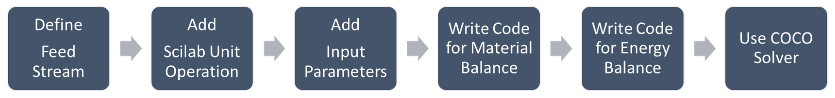
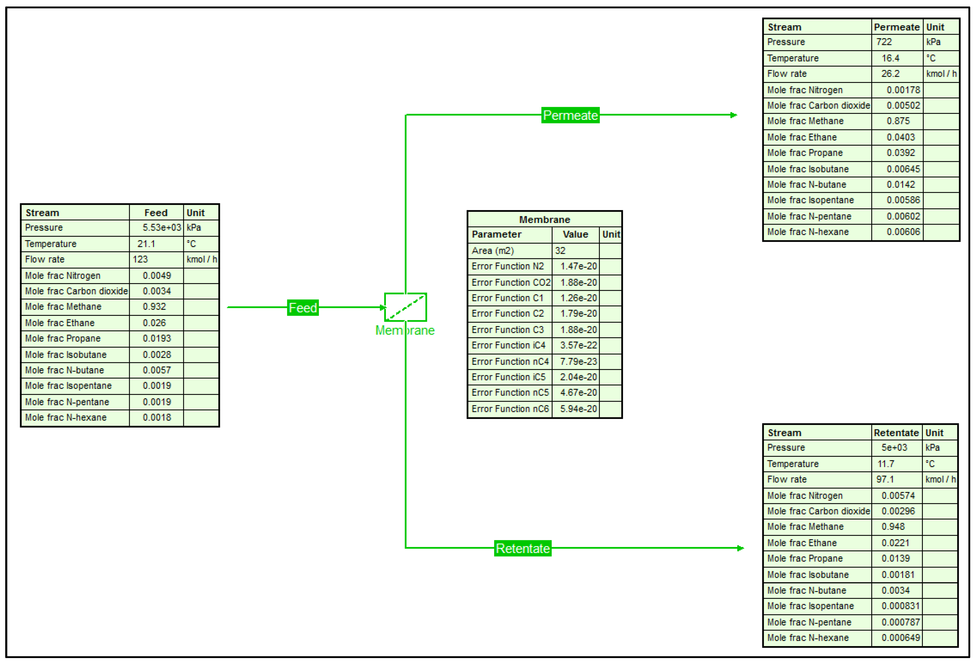
2.2. Membrane Development in COCO

In COCO, the membrane unit was built using the same equations from (1) to (11). However, the system was solved using the “fsolve” function from the external software, Scilab V6.1 (2024). First, the feed stream was defined in COCO but unlike UniSIM^®, the feed flowrate of 2.5 MMSCFD could not be entered directly. The flowrate was converted to kmol h⁻¹ by finding the gas density at a standard temperature of 15.5 °C and a standard pressure of 100 kPa (STP). The membrane unit was then added as a black box using the Scilab Unit Operation. After that, the equations were added in the Scilab script, and the streams were linked using the “getParameter” command.

Additional input data were added to the “Parameters” page of the Scilab plugin. The error function (Equation (11)) was added and solved using the “fsolve” command in Scilab. Unlike UniSIM^®, the unit operation of the Scilab plugin does not have energy balance equations. This is required to determine the temperature of the permeate due to the reduction in pressure. The following equation represents the energy balance across the membrane:

$$n_F{H}_F-n_P{H}_P-n_R{H}_R=0$$

(12)

where H is the enthalpy in kJ kmol⁻¹. The equation is solved numerically by guessing the permeate temperature. First, the permeate temperature is assumed to be equal to the feed temperature (isothermal system), and the “fsolve” command will solve Equation (12) by changing the permeate temperature. Figure 5 summarizes the steps for building a membrane unit in COCO using the Scilab unit operation. Part of the written Scilab script is shown in Figure 6.

The developed membrane units in UniSIM^® and COCO were evaluated with field data of a PDMS membrane reported by MTR. The simulation was used to calculate flowrates and compositions of permeate and retentate. The error was determined using the following formula:

$$\mathrm{Error} \left(\%\right)={\displaystyle \frac{\mathrm{Calculated} \mathrm{Value}-\mathrm{Reported} \mathrm{Value}}{\mathrm{Reported} \mathrm{Value}}} \times 100$$

(13)

The simulation was performed using a laptop PC equipped with core i7-4610M at 3 Ghz with 8 GB of physical memory (RAM).

3. Results and Discussion

The guessed permeate cuts were assumed as 0.5 for all components. Unfortunately, UniSIM^® could not solve the system and cuts were changed manually until the system was converged, and this took a few minutes to complete. However, for COCO, the membrane was solved using the first permeate cuts of 0.5, and it took only 7 s. This indicates COCO solved the membrane unit faster than UniSIM^®. Figure 7 shows the solved case in UniSIM^® while Figure 8 shows the solved sheet in COCO. The developed cases can be downloaded as Supplementary Files.

Table 2. Comparison between field data and calculated data from UniSIM^® and COCO for fuel gas conditioning by a PDMS membrane.

Property	Field Data [11]	UniSIM®	COCO
Permeate stream
Temperature (°C)	–	16.6	16.4
Flowrate (MMSCFD)	0.50	0.53	0.50
N2 (mol%)	0.76	0.18	0.18
CO2 (mol%)	0.48	0.49	0.50
C1 (mol%)	85.9	87.64	87.50
C2 (mol%)	4.13	3.97	4.03
C3 (mol%)	3.91	3.88	3.92
iC4 (mol%)	0.67	0.64	0.64
nC4 (mol%)	1.51	1.41	1.42
iC5 (mol%)	0.70	0.58	0.59
nC5 (mol%)	0.76	0.60	0.60
nC6 (mol%)	1.18	0.60	0.61
Retentate stream
Flowrate (MMSCFD)	2.0	2.0	2.0
N2 (mol%)	0.51	0.57	0.57
CO2 (mol%)	0.28	0.30	0.30
C1 (mol%)	94.30	94.75	94.78
C2 (mol%)	2.43	2.23	2.21
C3 (mol%)	1.46	1.40	1.39
iC4 (mol%)	0.21	0.18	0.18
nC4 (mol%)	0.41	0.34	0.34
iC5 (mol%)	0.13	0.08	0.08
nC5 (mol%)	0.14	0.08	0.08
nC6 (mol%)	0.13	0.07	0.06
Average Error (%)	–	17.4	17.1

shows the calculated flowrates and compositions of permeate and retentate compared to field data. UniSIM^® predictions have an error of 17.4% whereas COCO gives a slightly lower error of 17.1%. However, in both software, the error is considered a bit high because, in refinery processes, an error of 12% is usually acceptable [15]. Nevertheless, some researchers consider the error of 20% and less is still acceptable due to the complexity of the simulation [16,17,18].

One possible reason for the high error is the impact of plasticization and concentration polarization. In this study, it was assumed that the membrane did not suffer from these effects but in reality, the accumulation of non-permeable molecules with time can cause resistance to gas flow [19]. Furthermore, heavy hydrocarbons are known to cause swelling therefore altering the surface properties [20]. This will change the permeance values therefore increasing the error. For instance, in Table 2, the simulators predicted a higher methane concentration at the permeate, but in reality, methane composition decreased by the previously mentioned effects.

The slightly lower error in COCO compared to UniSIM^® is related to the lower value in error functions (Equation (11)). COCO has error functions in the range of 10⁻²⁰ while UniSIM^® has errors in the range of 10⁻⁶ as shown in Figure 7 and Figure 8. The “fsolve” function in Scilab solves better and faster compared to the adjust functions in UniSIM^®. This is because “fsolve” uses the trust-region algorithm while UniSIM^® uses the Levenberg–Marquardt method. It is reported that the trust-region method is a modified version of the Levenberg–Marquardt algorithm [21]. The trust-region method uses a defined region based on the difference between the guessed and calculated value while the Levenberg–Marquardt algorithm is general and uses a wider region [22].

By comparing UniSIM^® to COCO for building the membrane unit for fuel gas conditioning, the unit was easier to create in UniSIM^® because all the objects were available in the simulator. In COCO, more time was needed to develop the unit due to the need for external software with the use of coding. The feed data were entered directly in UniSIM^®, but in COCO, the data was converted manually due to the limitation of units. This is because UniSIM^® is designed for industrial applications whereas COCO targets academic users. Furthermore, energy balance equations were added in COCO while UniSIM^® performed energy balance automatically. The membrane process was solved in a few seconds in COCO with better accuracy compared to UniSIM^® due to the use of the trust-region method.

Table 3. Comparison between UniSIM^® and COCO for building a membrane unit for fuel gas conditioning.

Parameter	UniSIM®	COCO
Software license	Commercial	Free
Membrane unit elements	Component splitter Spreadsheet Adjust functions	Scilab plugin Program coding
Time to build unit	Short	Long
Units conversion	Automatically	Manually for feed flowrate
Mass balance	Need to add equations	Need to add equations
Heat balance	Automatically	Need to add equations
Need initial guesses to solve	Yes	Yes
Solved from first guess *	No	Yes
Solving time **	Few minutes (depending on initial guesses)	Few seconds
Error from field data	Higher	Lower

* Using permeate cut values of 0.5. ** Based on core i7-4610M laptop PC at 3 GHz with 8 GB RAM.

summarizes the difference between UniSIM^® and COCO for building the membrane unit for fuel gas conditioning. For faster simulation results, it is advised to use UniSIM^®, while it is recommended to use COCO for more accurate results.

4. Conclusions

Process simulators are used to predict the performance of unit operations. Unfortunately, most simulators lack a ready-to-use membrane unit for gas separation. In this work, a membrane unit was built in the commercial software UniSIM^® and the freeware application COCO. The developed units were assessed with field data of a PDMS membrane for fuel gas conditioning. The membrane unit was easier to develop in UniSIM^® due to the availability of tools such as component splitter and adjust functions. COCO required a longer time to build the unit, but it solved the system faster with better accuracy due to the use of the “fsolve” function in Scilab script. When calculating the flow rate and composition of all compounds, COCO gives an error of 17.1% while UniSIM^® resulted in a slightly higher error of 17.4%. The large error was related to the effects of plasticization and concentration polarization that were neglected in the mathematical model.

References

1. Gkotsis, P.; Peleka, E.; Zouboulis, A. Membrane-based technologies for post-combustion CO2 capture from flue gases: Recent progress in commonly employed membrane materials. Membranes 2023, 13, 898. [Google Scholar] [CrossRef] [PubMed]
2. Basile, A.; Favvas, E. Current Trends and Future Developments on (Bio-) Membranes; Elsevier: Amsterdam, The Netherlands, 2024; pp. 3–28. [Google Scholar]
3. He, X.; Lie, J.; Sheridan, E.; Hägg, M.-B. CO2 capture by hollow fibre carbon membranes: Experiments and process simulations. Energy Procedia 2009, 1, 261–268. [Google Scholar] [CrossRef]
4. Offord, G.; Armstrong, S.; Freeman, B.; Baer, E.; Hiltner, A.; Paul, D. Gas transport in coextruded multilayered membranes with alternating dense and porous polymeric layers. Polym 2014, 55, 1259–1266. [Google Scholar] [CrossRef]
5. Lahiri, S. Profit Maximization Techniques for Operating Chemical Plants; Wiley: Hoboken, NJ, USA, 2020. [Google Scholar]
6. Du, Z.; Li, C.; Sun, W.; Wang, J. A simulation of diesel hydrotreating process with real component method. Chin. J. Chem. Eng. 2015, 23, 780–788. [Google Scholar] [CrossRef]
7. Oyegoke, T. COCO, a process simulator: Methane oxidation simulation & its agreement with commercial simulator’s predictions. Chem. Prod. Process Model. 2023, 18, 995–1004. [Google Scholar]
8. Chemmangattuvalappil, N.; Chong, C.H.; Foo, D.C.Y.; Ng, D.K.S.; Elyas, R.; Chen, C.-L.; Chien, I.; Elms, R.D.; Lee, H.-Y.; Chong, S. Chemical Engineering Process Simulation; Elsevier Science: Amsterdam, The Netherlands, 2017. [Google Scholar]
9. Yeom, C.; Kim, J.; Park, H.; Lee, J.; Park, S.; Gu, B. Simulation model for prediction of gas separation in membrane contactor process. Membranes 2022, 12, 158. [Google Scholar] [CrossRef] [PubMed]
10. Mirzaee, H.; Mirzaee, F. Modeling and simulation gas separation by membrane of poly dimethyl siloxane. J. King Saud Univ.-Eng. Sci. 2012, 24, 35–43. [Google Scholar] [CrossRef]
11. Baker, R.; Hofmann, T.; Jariwala, A. Field Demonstration of a Membrane Process to Recover Heavy Hydrocarbons and to Remove Water From Natural Gas; United States Department of Energy: Washington, DC, USA, 2007. [Google Scholar]
12. Sethi, S.; Wiesner, M. Simulated cost comparisons of hollow-fiber and integrated nanofiltration configurations. Water Res. 2000, 34, 2589–2597. [Google Scholar] [CrossRef]
13. Wenten, I.; Recent Development in Membrane and Its Industrial Applications. Membrane Technology in Oil and Gas Industry; 2005, Indonesia 2005. Available online: https://www.researchgate.net/publication/281257916_Recent_Development_in_Membrane_and_Its_Industrial_Applications_Membrane_Technology_in_Oil_and_Gas_Industry (accessed on 19 October 2024).
14. Davis, R. Simple gas permeation and pervaporation membrane unit operation models for process simulators. Chem. Eng. Technol. 2002, 25, 717–722. [Google Scholar] [CrossRef]
15. Ahmad, Z. Recent Trends in Processing and Degradation of Aluminium Alloys; IntechOpen: London, UK, 2011. [Google Scholar]
16. Triantafyllidis, T. Holistic Simulation of Geotechnical Installation Processes: Numerical and Physical Modelling; Springer International Publishing: Manhattan, NY, USA, 2015. [Google Scholar]
17. Bafleur, M.; Caignet, F.; Nolhier, N. ESD Protection Methodologies: From Component to System; Elsevier Science: Amsterdam, The Netherlands, 2017. [Google Scholar]
18. Koh, H.; Teh, S. Ecological Modeling for Mitigating Environmental and Climate Shocks: Achieving the UNSDGs; World Scientific Publishing Company: Singapore, 2021. [Google Scholar]
19. Drioli, E.; Barbieri, G.; Peter, L.M. Membrane Engineering for the Treatment of Gases: Gas-Separation Problems with Membranes; Royal Society of Chemistry: London, UK, 2011. [Google Scholar]
20. Ismail, A.; Khulbe, K.; Matsuura, T. Gas Separation Membranes: Polymeric and Inorganic; Springer International Publishing: Manhattan, NY, USA, 2015. [Google Scholar]
21. Conn, A.; Gould, N.; Toint, P. Trust Region Methods; Society for Industrial and Applied Mathematics: Philadelphia, PA, USA, 2000. [Google Scholar]
22. Marsland, S. Machine Learning: An Algorithmic Perspective; CRC Press: Boca Raton, FL, USA, 2014. [Google Scholar]
Figure 1. Streams of a cross-flow membrane unit for fuel gas conditioning.
Eng 05 00164 g001
Figure 2. Required input data for solving the membrane system and the calculated outputs.
Eng 05 00164 g002
Figure 3. Steps in UniSIM® for building and solving a membrane unit for gas separation.
Eng 05 00164 g003
Figure 4. Screenshot of the developed UniSIM® spreadsheet for simulating a membrane unit for gas separation.
Eng 05 00164 g004
Figure 5. Steps in COCO and Scilab for building a membrane unit for gas separation.
Eng 05 00164 g005
Figure 6. Screenshot of the written code in Scilab plugin for simulating the membrane unit in COCO for fuel gas conditioning.
Eng 05 00164 g006
Figure 7. Solved process flow sheet in UniSIM® for fuel gas conditioning by a membrane.
Eng 05 00164 g007
Figure 8. Solved process flow sheet in COCO using Scilab plugin for fuel gas conditioning by a PDMS membrane.
Eng 05 00164 g008