
Artificial Intelligence-Based Techniques for Fouling Resistance Estimation of Shell and Tube Heat Exchanger: Cascaded Forward and Recurrent Models

 ,
,  , , ,
, , ,  , and
, and 
Abstract
:1. Introduction
- Efficient Model Design: the proposed models utilize only six input parameters, reducing complexity while maintaining accuracy.
- High-Precision Training: the Levenberg–Marquardt algorithm ensures rapid convergence and minimizes mean squared error (MSE).
- Robust Validation: the models’ generalization ability is tested using external datasets.
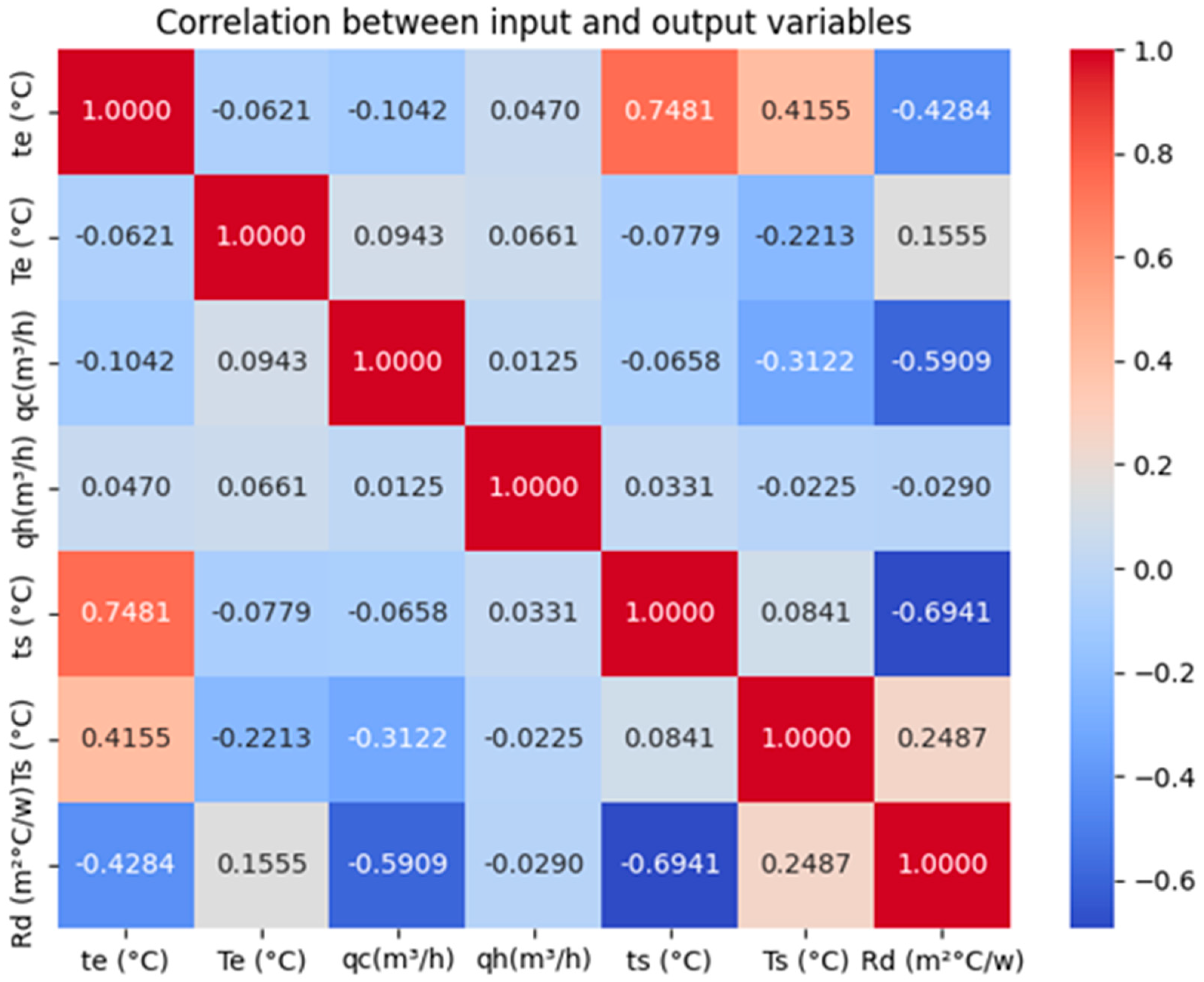
- Correlation Analysis: the relationships between input variables and fouling resistance are thoroughly analyzed.
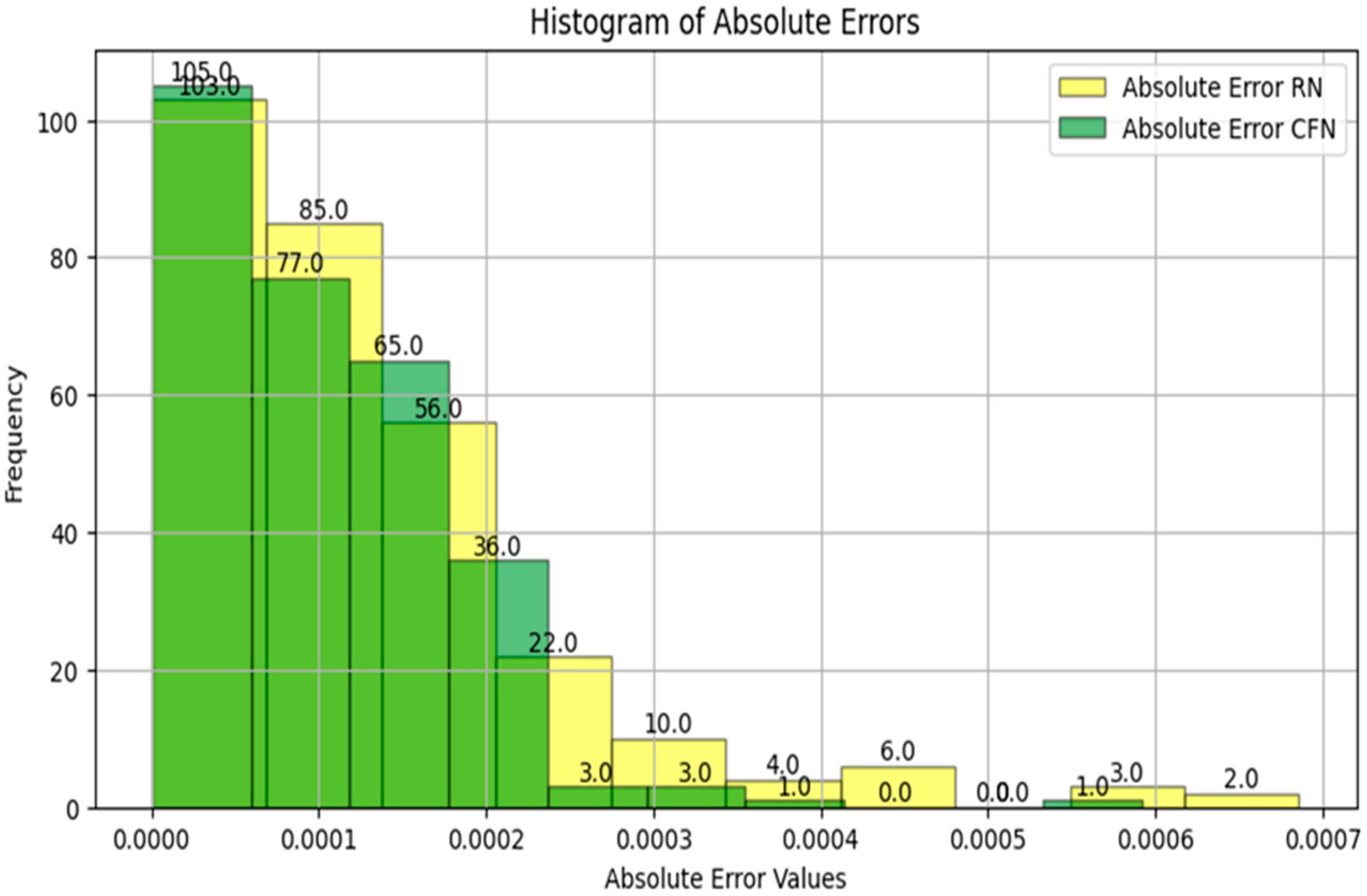
- Statistical Performance Evaluation: error metrics, absolute error histograms, and descriptive statistics provide insight into model reliability and accuracy.
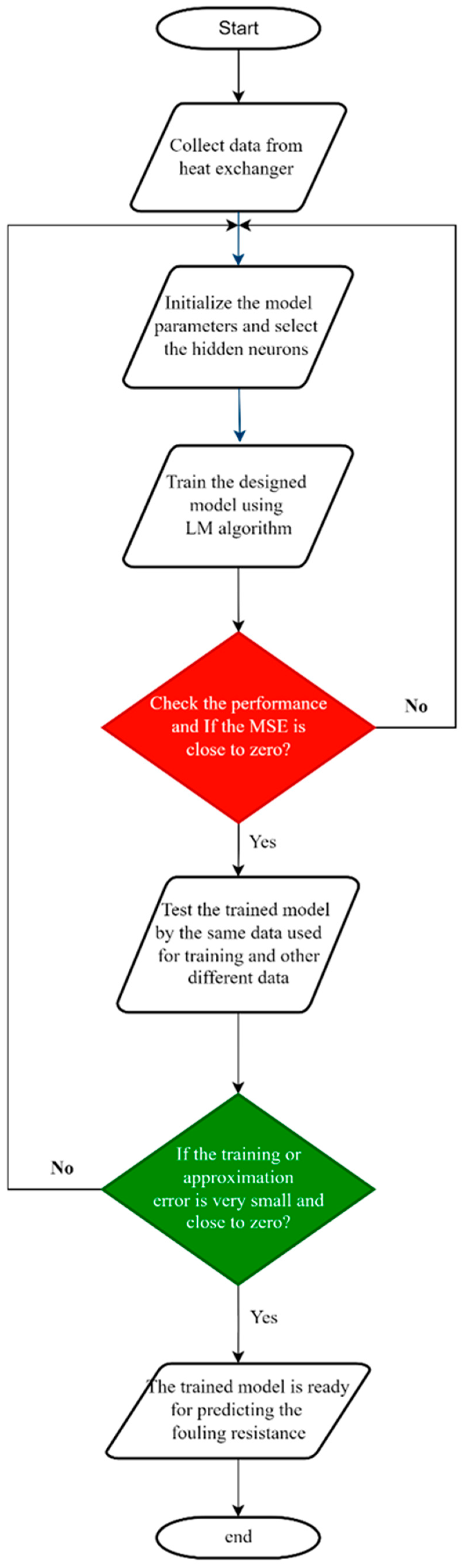
2. Materials and Methods
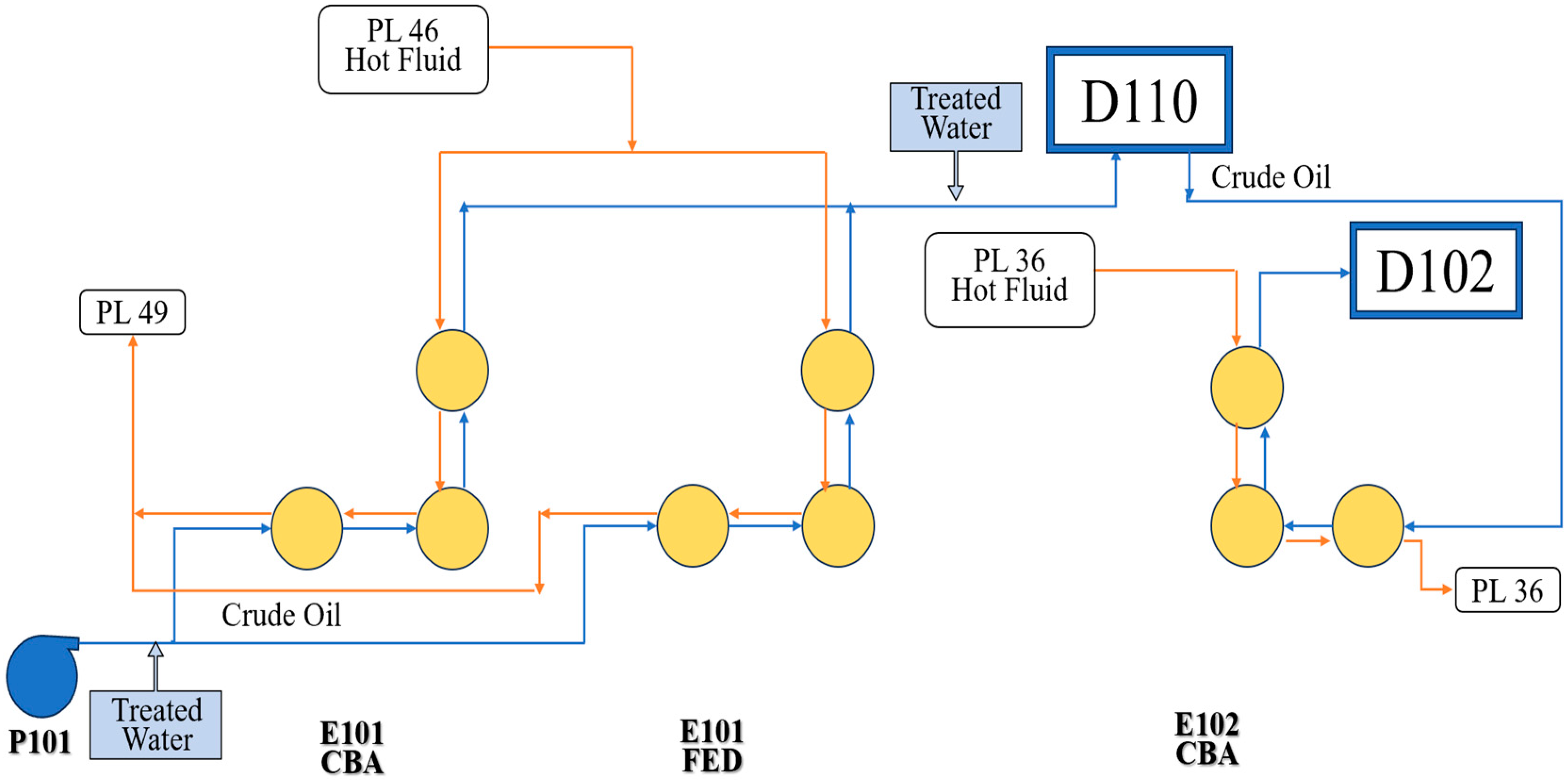
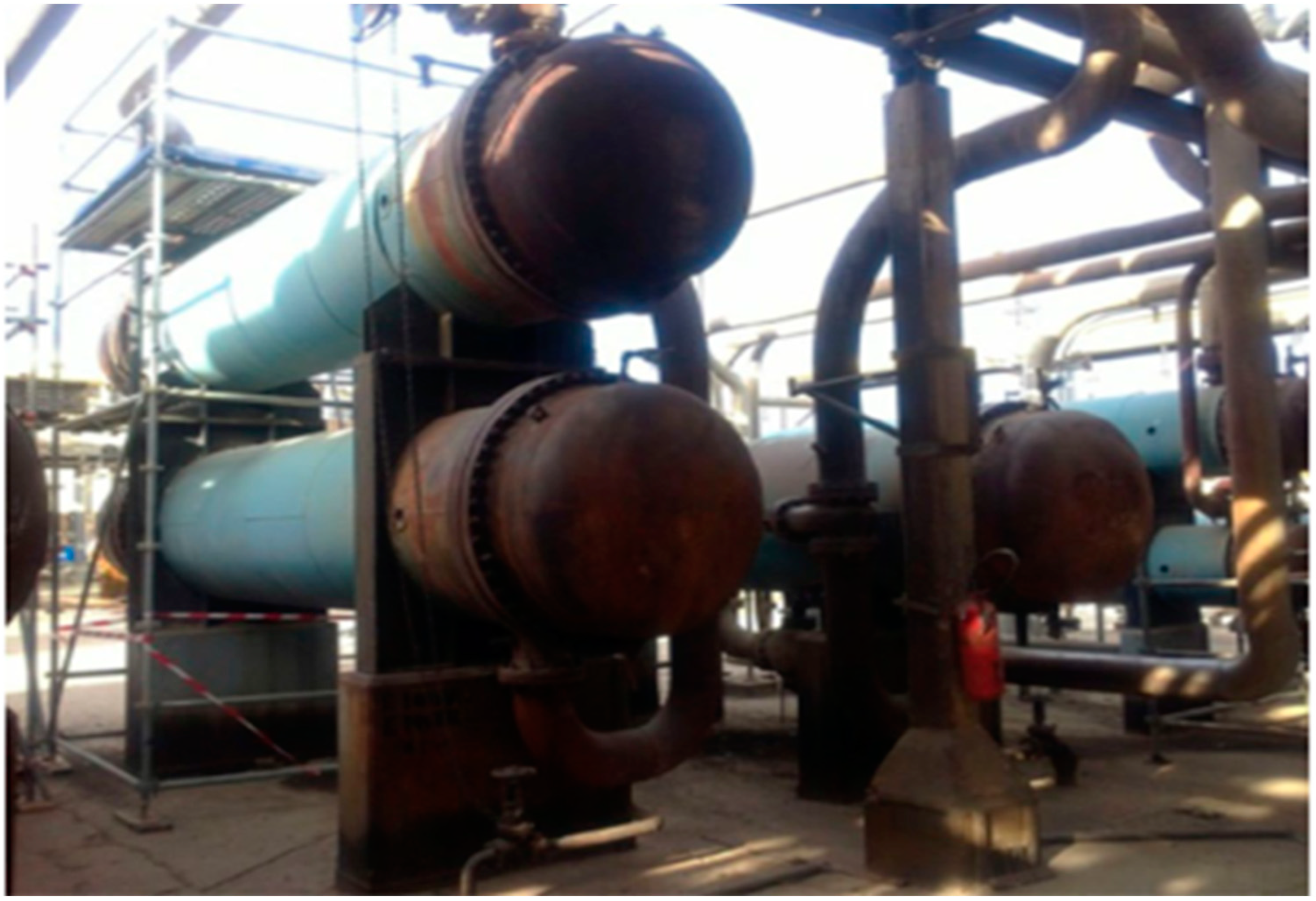
2.1. Experimental Procedure
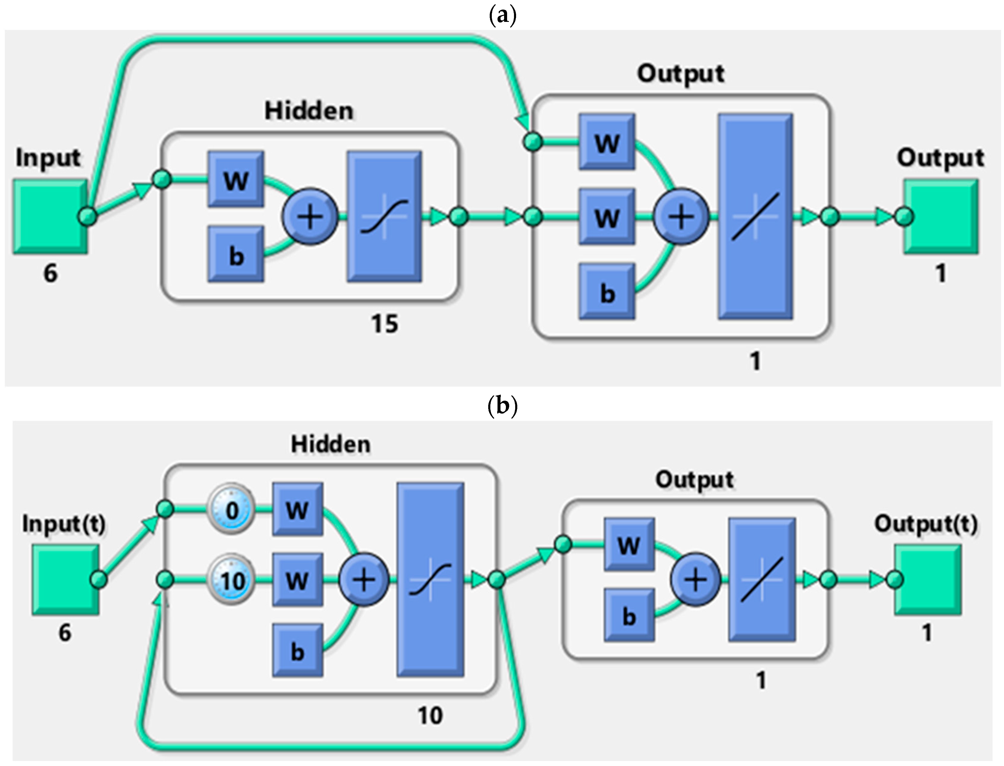
2.2. Neural Networks Structures
3. Results
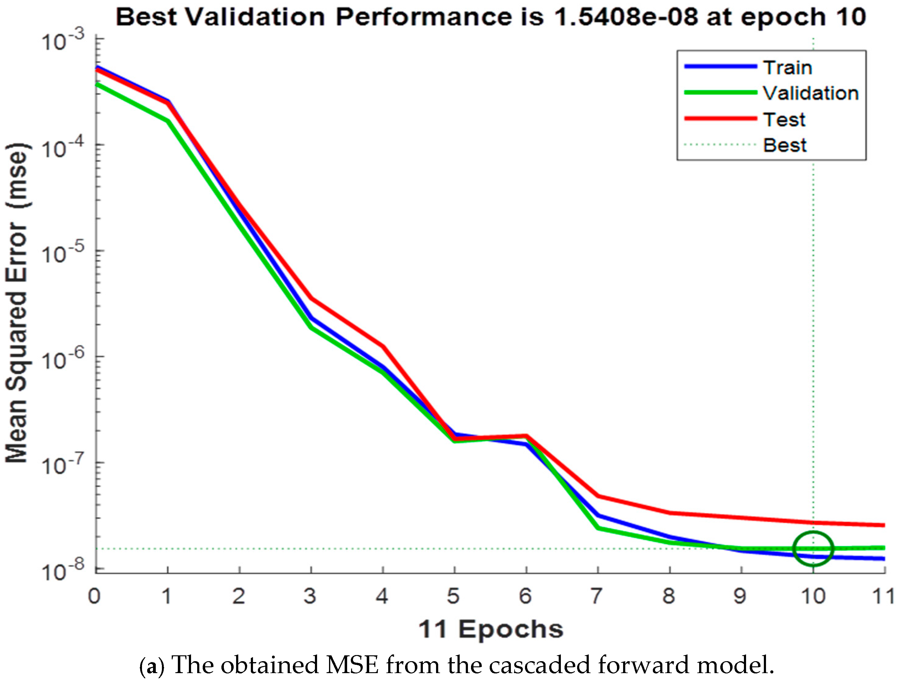
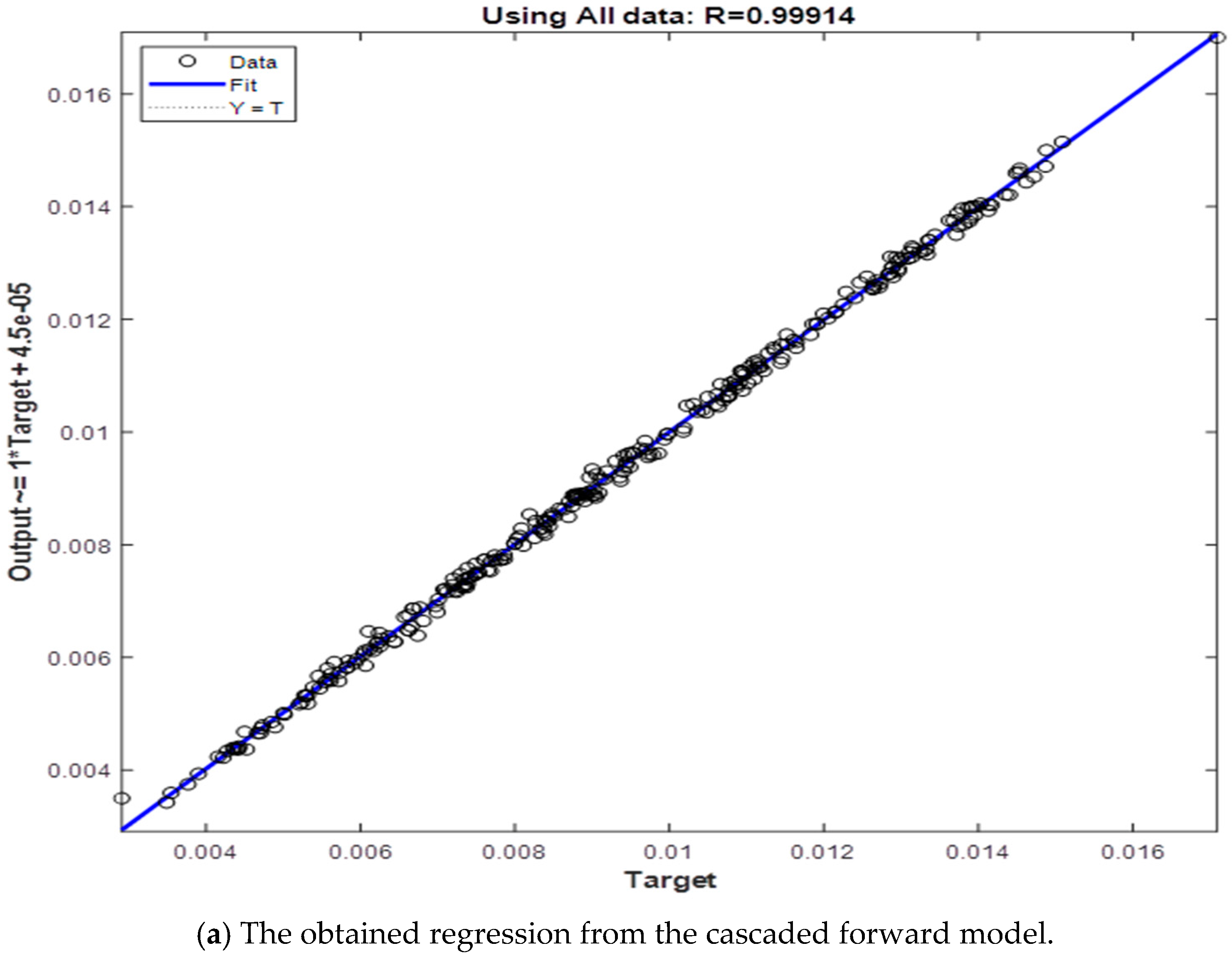
3.1. Results from Training Stage
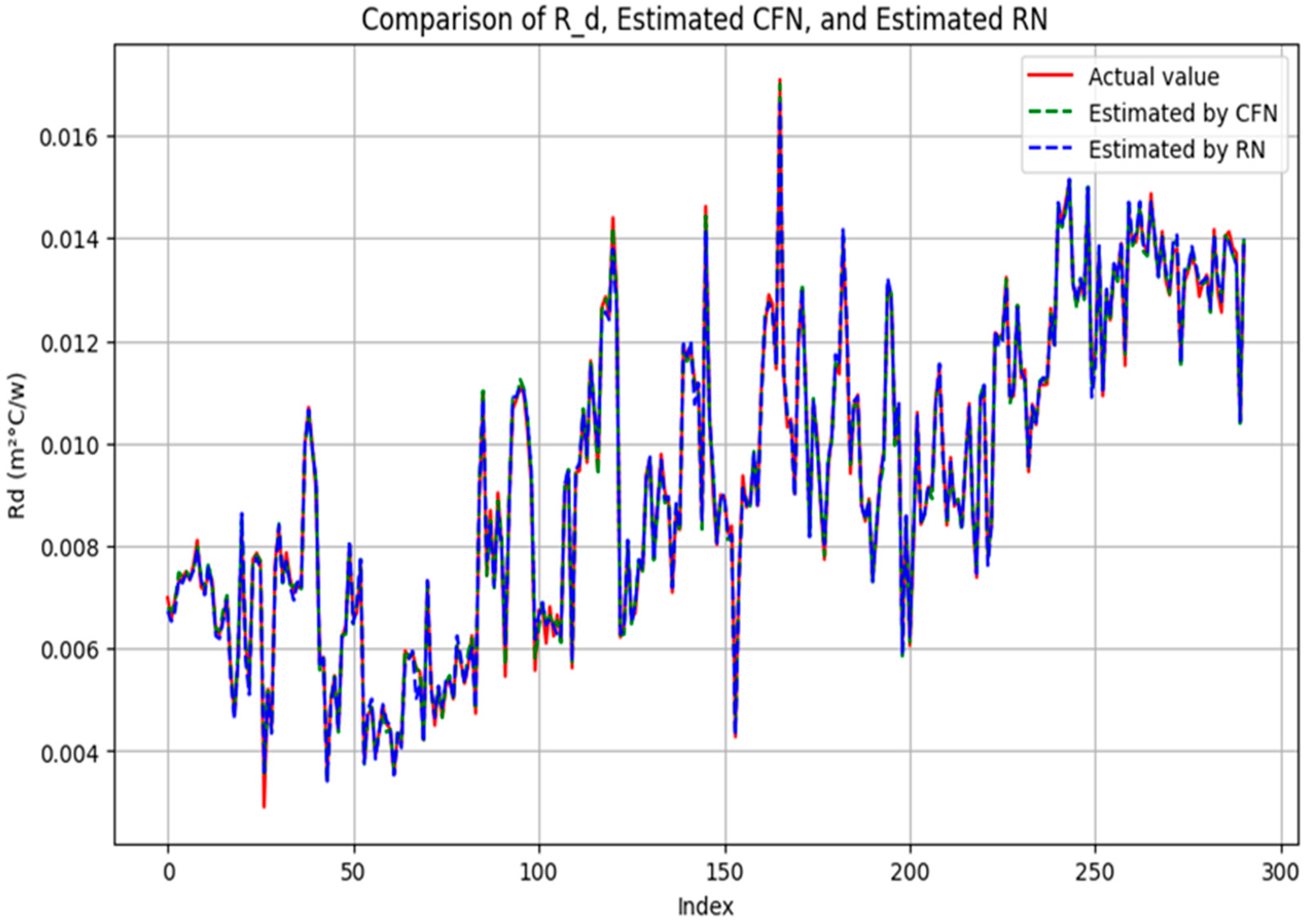
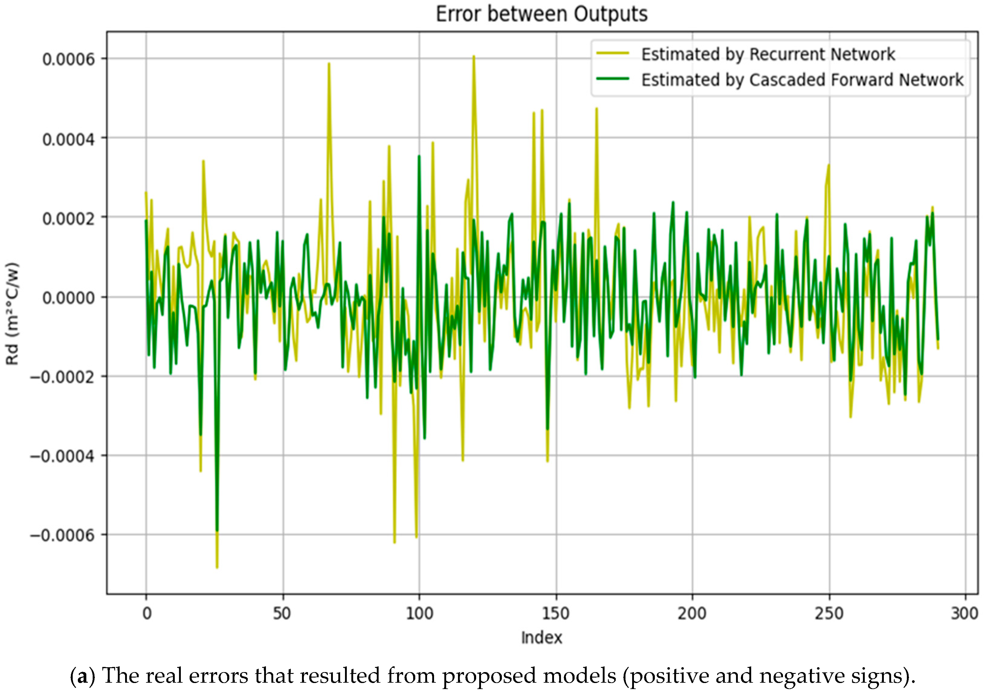
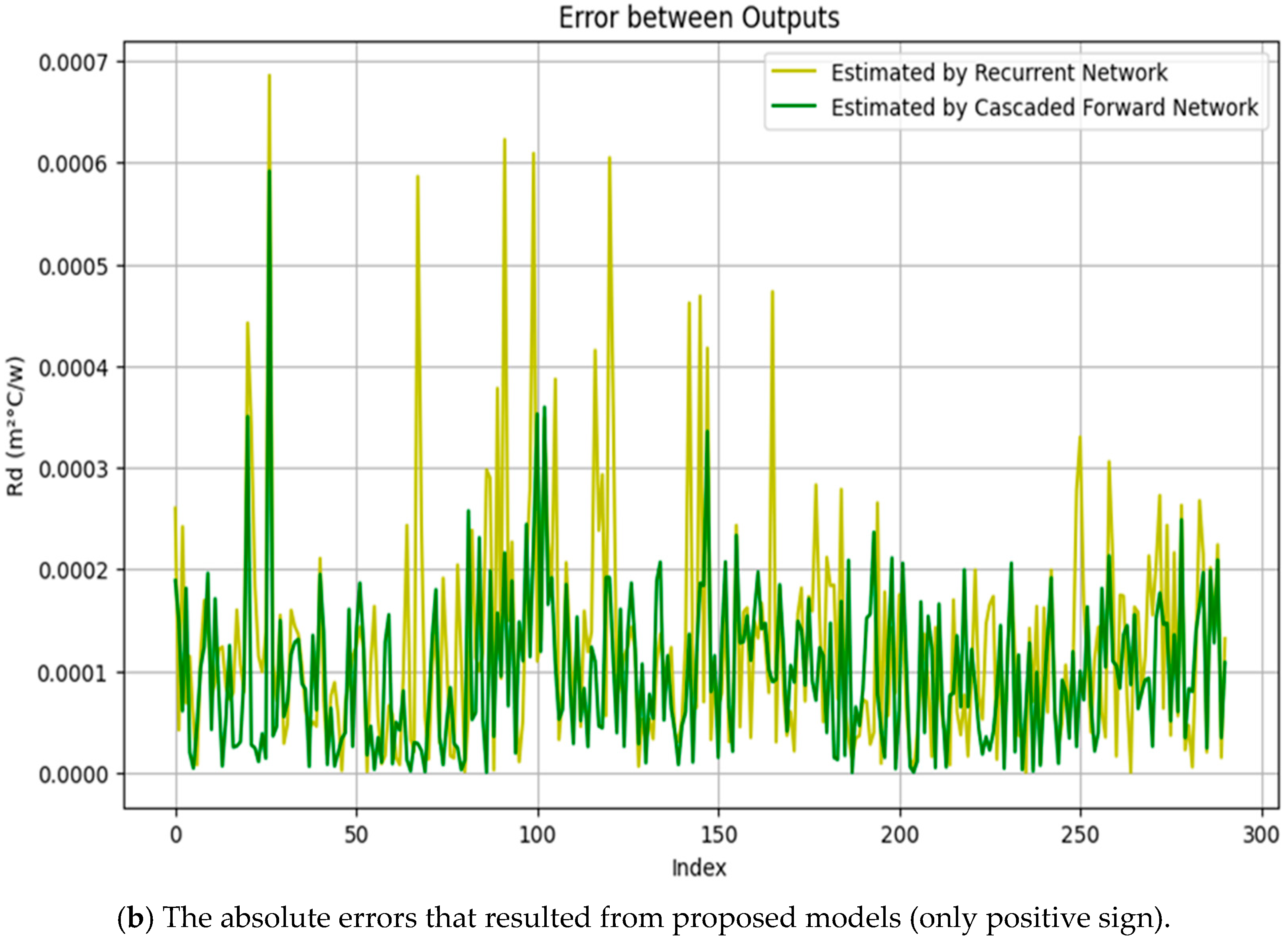
3.2. Results from Verification Stage
Statistical Analysis of Performance Differences
4. Discussion
4.1. Correlation Between Input Variables
4.2. Error Histogram
4.3. Descriptive Statistical Analysis
4.4. Comparison with Other Models
5. Conclusions and Future Work
Author Contributions
Funding
Institutional Review Board Statement
Informed Consent Statement
Data Availability Statement
Conflicts of Interest
References
- Olympios, A.V.; McTigue, J.D.; Farres-Antunez, P.; Tafone, A.; Romagnoli, A.; Li, Y.; Ding, Y.; Steinmann, W.-D.; Wang, L.; Chen, H.; et al. Progress and prospects of thermo-mechanical energy storage—A critical review. Prog. Energy 2021, 3, 22001. [Google Scholar] [CrossRef]
- Tavousi, E.; Perera, N.; Flynn, D.; Hasan, R. Heat transfer and fluid flow characteristics of the passive method in double tube heat exchangers: A critical review. Int. J. Thermofluids 2023, 17, 100282. [Google Scholar] [CrossRef]
- Roy, U.; Majumder, M. Economic optimization and energy analysis in shell and tube heat exchanger by meta-heuristic approach. Vacuum 2019, 166, 413–418. [Google Scholar] [CrossRef]
- Delrot, S.; Guerra, T.M.; Dambrine, M.; Delmotte, F. Fouling detection in a heat exchanger by observer of, Takagi-Sugeno type for systems with unknown polynomial inputs. Eng. Appl. Artif. Intell. 2012, 25, 1558–1566. [Google Scholar] [CrossRef]
- Musawel, R.K. Simulation and Fouling Study of Propane Heat Exchangers. Master’s Thesis, University of Basrah, Basrah, Iraq, 2002. [Google Scholar]
- Coletti, F.; Hewitt, G. Crude Oil Fouling: Deposit Characterization, Measurements, and Modeling; Gulf Professional Publishing: Woburn, MA, USA, 2014. [Google Scholar]
- Diaz-Bejarano, E.; Behranvand, E.; Coletti, F.; Mozdianfard, M.R.; Macchietto, S. Organic and inorganic fouling in heat exchangers: Industrial case study analysis of fouling rate. Ind. Eng. Chem. Res. 2018, 58, 228–246. [Google Scholar] [CrossRef]
- Al Hadad, W.; Schick, V.; Maillet, D. Fouling detection in a shell and tube heat exchanger using variation of its thermal impulse responses: Methodological approach and numerical verification. Appl. Therm. Eng. 2019, 155, 612–619. [Google Scholar] [CrossRef]
- Das, S.; O’Connell, M.G.; Xu, H.; Bernstein, R.; Kim, J.-H.; Sankhala, K.; Segal-Peretz, T.; Shevate, R.; Zhang, W.; Zhou, X.; et al. Assessing advances in anti-fouling membranes to improve process economics and sustainability of water treatment. ACS EST Eng. J. 2022, 2, 2159–2173. [Google Scholar] [CrossRef]
- Ikram, K.; Djilali, K.; Abdennasser, D.; Al-Sabur, R.; Ahmed, B.; Sharkawy, A.-N. Comparative analysis of fouling resistance prediction in shell and tube heat exchangers using advanced machine learning techniques. Res. Eng. Struct. Mater. 2023, 10, 253–270. [Google Scholar] [CrossRef]
- Berce, J.; Zupančič, M.; Može, M.; Golobič, I. Infrared thermography observations of crystallization fouling in a plate heat exchanger. Appl. Therm. Eng. 2023, 224, 120116. [Google Scholar] [CrossRef]
- Fawait, A.B.; Rahmah, S.; da Costa, A.D.S.; Insyroh, N.; Firdaus, A.A. Implementation of Data Mining Using Simple Linear Regression Algorithm to Predict Export Values. Sci. J. Eng. Res. 2025, 1, 26–32. [Google Scholar]
- Sharkawy, A.N. Principle of neural network and its main types. J. Adv. Appl. Comput. Math. 2020, 7, 8–19. [Google Scholar] [CrossRef]
- Davoudi, E.; Vaferi, B. Applying artificial neural networks for systematic estimation of degree of fouling in heat exchangers. Chem. Eng. Res. Des. 2018, 130, 138–153. [Google Scholar] [CrossRef]
- Ben-Mansour, R.; El-Ferik, S.; Al-Naser, M.; Qureshi, B.A.; Eltoum, M.A.M.; Abuelyamen, A.; Al-Sunni, F.; Ben Mansour, R. Experimental/Numerical Investigation and Prediction of Fouling in Multiphase Flow Heat Exchangers: A Review. Energies 2023, 16, 2812. [Google Scholar] [CrossRef]
- Zheng, X.; Yang, R.; Wang, Q.; Yan, Y.; Zhang, Y.; Fu, J.; Liu, Z. Comparison of GRNN and RF algorithms for predicting heat transfer coefficient in heat exchange channels with bulges. Appl. Therm. Eng. 2022, 217, 119263. [Google Scholar] [CrossRef]
- Panda, J.P.; Kumar, B.; Patil, A.K.; Kumar, M.; Kumar, R. Machine learning assisted modeling of thermohydraulic correlations for heat exchangers with twisted tape inserts. Acta Mech. Sin. 2023, 39, 322036. [Google Scholar] [CrossRef]
- Gupta, A.K.; Kumar, P.; Sahoo, R.K.; Sahu, A.K.; Sarangi, S.K. Performance measurement of plate fin heat exchanger by exploration: ANN, ANFIS, GA, and SA. J. Comput. Des. Eng. 2017, 4, 60–68. [Google Scholar] [CrossRef]
- Roy, U.; Majumder, M. Evaluating heat transfer analysis in heat exchanger using, NN with, IGWO algorithm. Vacuum 2019, 161, 186–193. [Google Scholar] [CrossRef]
- Muthukrishnan, S.; Krishnaswamy, H.; Thanikodi, S.; Sundaresan, D.; Venkatraman, V. Support vector machine for modeling and simulation of heat exchangers. Therm. Sci. 2020, 24, 499–503. [Google Scholar] [CrossRef]
- Kumra, A.; Rawal, N.; Samui, P. Prediction of heat transfer rate of a, Wire-on-Tube type heat exchanger: An, Artificial, Intelligence approach. Procedia Eng. 2013, 64, 74–83. [Google Scholar] [CrossRef]
- Wen, X.Q. Study on the methods of predicting the fouling characteristics of plate heat exchanger based on water quality parameters. Appl. Mech. Mater. 2013, 459, 153–158. [Google Scholar] [CrossRef]
- El-Said, E.M.S.; Abd Elaziz, M.; Elsheikh, A.H. Machine learning algorithms for improving the prediction of air injection effect on the thermohydraulic performance of shell and tube heat exchanger. Appl. Therm. Eng. 2021, 185, 116471. [Google Scholar] [CrossRef]
- Shengxian, C.; Yanhui, Z.; Jing, Z.; Dayu, Y. Experimental Study on Dynamic Simulation for Biofouling Resistance Prediction by Least Squares Support Vector Machine. Energy Procedia 2012, 17, 74–78. [Google Scholar] [CrossRef]
- Mohanty, D.K. Application of neural network model for predicting fouling behaviour of a shell and tube heat exchanger. Int. J. Ind. Syst. Eng. 2017, 26, 228. [Google Scholar] [CrossRef]
- Sundar, S.; Rajagopal, M.C.; Zhao, H.; Kuntumalla, G.; Meng, Y.; Chang, H.C.; Shao, C.; Ferreira, P.; Miljkovic, N.; Sinha, S.; et al. Fouling modeling and prediction approach for heat exchangers using deep learning. Int. J. Heat Mass Transf. 2020, 159, 120112. [Google Scholar] [CrossRef]
- Kuzucanlı, S.A.; Vatansever, C.; Yaşar, A.E.; Karadeniz, Z.H. Assessment of fouling in Plate Heat exchangers using classification machine learning algorithms. In Proceedings of the CLIMA 2022 The 14th REHVA HVAC World Congress, Rotterdam, The Netherlands, 22–25 May 2022. [Google Scholar] [CrossRef]
- Hosseini, S.; Khandakar, A.; Ayari, M.A.; Rahman, T.; Chowdhury, M.H.; Vaferi, B. Novel and robust machine learning approach for estimating the fouling factor in heat exchangers. Energy Rep. 2022, 8, 8767–8776. [Google Scholar] [CrossRef]
- Harche, R.; Mouheb, A. The fouling in the crude distillation preheat train of Algerian refinery. Acta Period. Technol. 2022, 53, 272–284. [Google Scholar] [CrossRef]
- Al-Naser, M.; El-Ferik, S.; Ben Mansour, R.; AlShammari, H.Y.; AlAmoudi, A. Intelligent Prediction Approach of Fouling Location in Shell and Tube Heat Exchanger. In Proceedings of the 2020 IEEE 10th International Conference on System Engineering and Technology (ICSET), Shah Alam, Malaysia, 9 November 2020; pp. 139–144. [Google Scholar] [CrossRef]
- Ilyunin, O.; Bezsonov, O.; Rudenko, S.; Serdiuk, N.; Udovenko, S.; Kapustenko, P.; Arsenyeva, O. The neural network approach for estimation of heat transfer coefficient in heat exchangers considering the fouling formation dynamic. Therm. Sci. Eng. Prog. 2024, 51, 102615. [Google Scholar] [CrossRef]
- Harche, R.; Mouheb, A.; Absi, R. The fouling in the tubular heat exchanger of Algiers refinery. Heat Mass Transf. 2016, 52, 947–956. [Google Scholar] [CrossRef]
- Sharkawy, A.N.; Ameen, A.G.; Mohamed, S.; Abdel-Jaber, G.T.; Hamdan, I. Design, assessment, and modeling of multi-input single-output neural network types for the output power estimation in wind turbine farms. Automation 2024, 5, 190–212. [Google Scholar] [CrossRef]
- Sharkawy, A.N.; Ali, M.M.; Mousa, H.H.; Ali, A.S.; Abdel-Jaber, G.T.; Hussein, H.S.; Ismeil, M.A. Solar PV power estimation and upscaling forecast using different artificial neural networks types: Assessment, validation, and comparison. IEEE Access 2023, 11, 19279–19300. [Google Scholar] [CrossRef]
- Tong, S.; Zhang, X.; Tong, Z.; Wu, Y.; Tang, N.; Zhong, W. Online ash fouling prediction for boiler heating surfaces based on wavelet analysis and support vector regression. Energies 2019, 13, 59. [Google Scholar] [CrossRef]
- Jradi, R.; Marvillet, C.; Jeday, M.R. Application of an artificial neural networks method for the prediction of the tube-side fouling resistance in a shell-and-tube heat exchanger. Fluid Dyn. Mater. Process. 2022, 18, 1511–1519. [Google Scholar] [CrossRef]


| Construction Material | Carbon Steel |
|---|---|
| Shell Diameter (m) | 1.067 |
| Baffle Spacing (m) | 0.465 |
| Number of Shells | 3.000 |
| Tube Outer Diameter (m) | 0.020 |
| Tube Thickness (m) | BGW14 |
| Tube Length (m) | 5.740 |
| Total Number of Tubes | 6600.000 |
| Pitch: Staggered (m) | 0.025 |
| Total Heat Exchange Surface Area (m2) | 2322.770 |
| Overall Heat Transfer Coefficient (kW/m2 °C) | 36.680 |
| Parameter | Shell Side | Tube Side |
|---|---|---|
| Circulating Fluid | Head Reflux | Crude Oil |
| Mass Flow Rates (kg/s) | 126.000 | 90.120 |
| Viscosity (m2/s) Inlet/Outlet | - | 2.4 × 10⁻⁶–9.6 × 10⁻⁷ |
| Inlet Temperature (K) | 388.706 | 299.817 |
| Outlet Temperature (K) | 338.706 | 377.594 |
| Number of Passes | 1.000 | 4.000 |
| Fouling Factor | 0.001 | 0.002 |
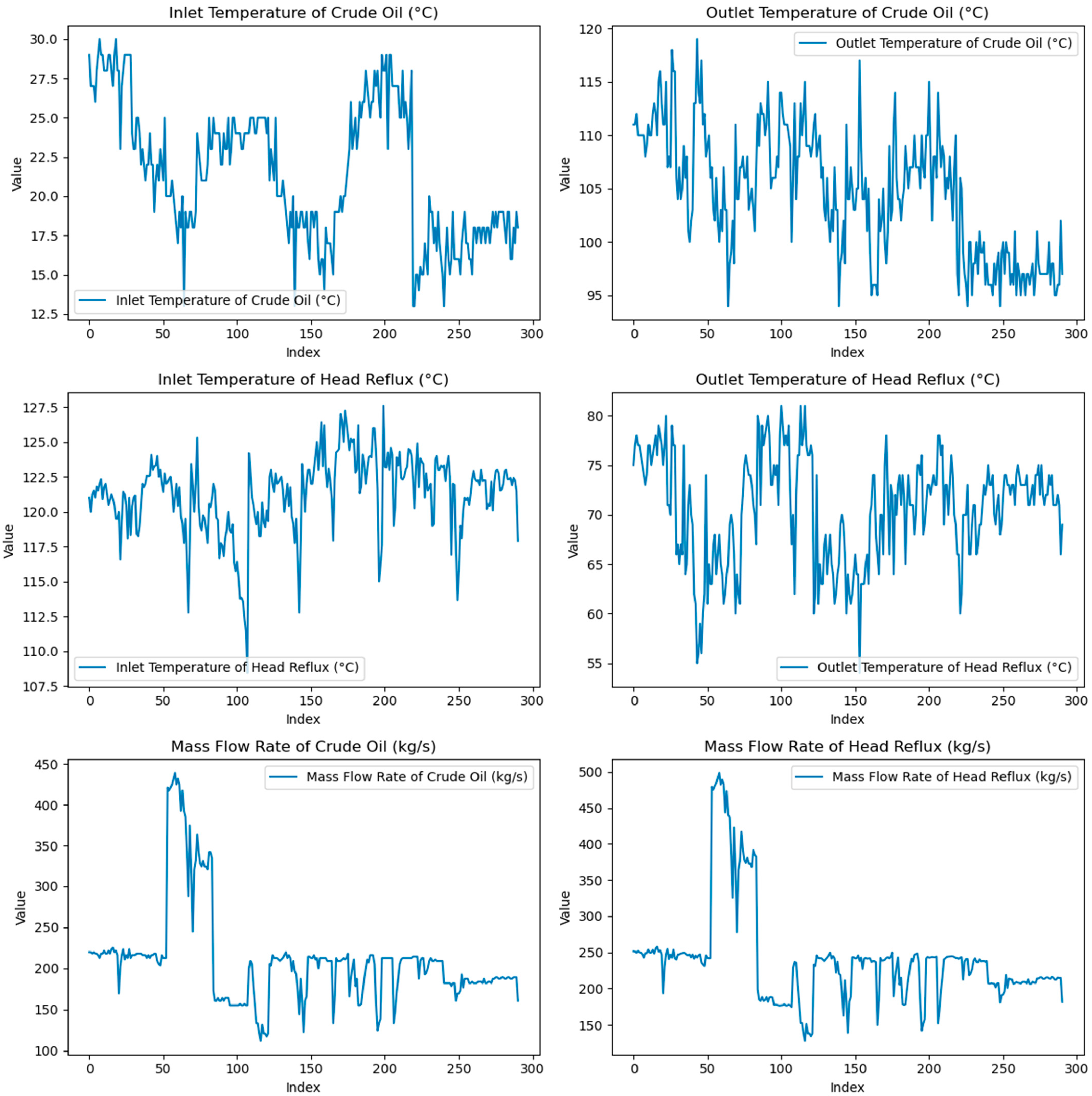
| Variables | Symbol | Range |
|---|---|---|
| Inlet Temperature of Crude Oil (°C) | te | 13–30 |
| Outlet Temperature of Crude Oil (°C) | ts | 94–119 |
| Inlet Temperature of Head Reflux (°C) | Te | 108.42–127.6 |
| Outlet Temperature of Head Reflux (°C) | Ts | 54–84 |
| Mass Flow Rate of Crude Oil (kg/s) | ṁt | 111.6–439.2 |
| Mass Flow Rate of Head Reflux (kg/s) | ṁc | 127.73–499 |
| Row | te | ts | Te | Ts | ṁt | ṁc |
|---|---|---|---|---|---|---|
| 1 | 29.00 | 111.00 | 121.00 | 75.00 | 219.60 | 251.29 |
| 2 | 27.00 | 111.00 | 120.00 | 77.00 | 219.60 | 251.03 |
| 3 | 27.00 | 112.00 | 121.25 | 78.00 | 217.80 | 249.24 |
| 4 | 27.00 | 110.00 | 121.50 | 77.00 | 219.60 | 251.91 |
| 5 | 26.00 | 110.00 | 121.00 | 77.00 | 217.80 | 249.71 |
| 6 | 28.00 | 110.00 | 121.80 | 76.00 | 217.80 | 249.49 |
| 7 | 29.00 | 110.00 | 121.50 | 75.00 | 216.00 | 247.11 |
| 8 | 30.00 | 110.00 | 122.00 | 74.00 | 212.40 | 242.44 |
| 9 | 29.00 | 108.00 | 122.33 | 73.00 | 217.80 | 248.82 |
| 10 | 29.00 | 109.00 | 120.90 | 74.00 | 217.80 | 248.66 |
| … | … | … | … | … | … | … |
| 291 | 18.00 | 97.00 | 117.90 | 69.00 | 160.20 | 181.29 |
| Refs. | Prediction Variable | Model Type | Evaluation Index |
|---|---|---|---|
| Tong et al. [35] | Ash fouling resistance | Support Vector Machine (SVM) | R = 0.985 |
| Davoudi and Vaferi. [14] | Fouling resistance in heat exchanger | Artificial Neural Network with MLP | R2 = 0.978 |
| Hossain et al. [28] | Fouling factor | Gaussian Process Regression (GPR) | R2 = 0.988 |
| Jradi et al. [36] | Fouling Resistance | Artificial Neural Network (ANN) | R2 = 0.994 |
| Present work | Fouling resistance | Cascaded forward network (CFN) and the recurrent neural network (RN) | R = 0.999 |
Disclaimer/Publisher’s Note: The statements, opinions and data contained in all publications are solely those of the individual author(s) and contributor(s) and not of MDPI and/or the editor(s). MDPI and/or the editor(s) disclaim responsibility for any injury to people or property resulting from any ideas, methods, instructions or products referred to in the content. |
© 2025 by the authors. Licensee MDPI, Basel, Switzerland. This article is an open access article distributed under the terms and conditions of the Creative Commons Attribution (CC BY) license (https://creativecommons.org/licenses/by/4.0/).
Share and Cite
Kouidri, I.; Dahmani, A.; Furizal, F.; Ma’arif, A.; Mostfa, A.A.; Amrane, A.; Mouni, L.; Sharkawy, A.-N. Artificial Intelligence-Based Techniques for Fouling Resistance Estimation of Shell and Tube Heat Exchanger: Cascaded Forward and Recurrent Models. Eng 2025, 6, 85. https://doi.org/10.3390/eng6050085
Kouidri I, Dahmani A, Furizal F, Ma’arif A, Mostfa AA, Amrane A, Mouni L, Sharkawy A-N. Artificial Intelligence-Based Techniques for Fouling Resistance Estimation of Shell and Tube Heat Exchanger: Cascaded Forward and Recurrent Models. Eng. 2025; 6(5):85. https://doi.org/10.3390/eng6050085
Chicago/Turabian StyleKouidri, Ikram, Abdennasser Dahmani, Furizal Furizal, Alfian Ma’arif, Ahmed A. Mostfa, Abdeltif Amrane, Lotfi Mouni, and Abdel-Nasser Sharkawy. 2025. "Artificial Intelligence-Based Techniques for Fouling Resistance Estimation of Shell and Tube Heat Exchanger: Cascaded Forward and Recurrent Models" Eng 6, no. 5: 85. https://doi.org/10.3390/eng6050085
APA StyleKouidri, I., Dahmani, A., Furizal, F., Ma’arif, A., Mostfa, A. A., Amrane, A., Mouni, L., & Sharkawy, A.-N. (2025). Artificial Intelligence-Based Techniques for Fouling Resistance Estimation of Shell and Tube Heat Exchanger: Cascaded Forward and Recurrent Models. Eng, 6(5), 85. https://doi.org/10.3390/eng6050085