Article

Lurie Control Systems Applied to the Sudden Cardiac Death Problem Based on Chua Circuit Dynamics

by
Rafael F. Pinheiro
1,*,
Diego Colón
2,
Alexandre Antunes
1,3 and
Rui Fonseca-Pinto
1,4
1
Center for Innovative Care and Health Technology (ciTechCare), School of Health Sciences (ESSLei), Polytechnic University of Leiria, 2414-016 Leiria, Portugal
2
Laboratory of Automation and Control (LAC), Telecommunications and Control Department, Polytechnic School, University of São Paulo, São Paulo 05508-010, Brazil
3
Life and Health Sciences Research Institute (ICVS), School of Medicine, University of Minho, 4710-057 Braga, Portugal
4
Instituto de Telecomunicações (IT), 2411-901 Leiria, Portugal
*
Author to whom correspondence should be addressed.
Submission received: 30 December 2024 / Revised: 14 April 2025 / Accepted: 22 April 2025 / Published: 25 April 2025
(This article belongs to the Section Electrical and Electronic Engineering)

Abstract

:
Sudden cardiac death (SCD) represents a critical public health challenge, emphasizing the need for predictive techniques that model complex physiological dynamics. Studies indicate that the “V-trough” pattern in sympathetic nerve activity (SNA) could act as an early indicator of potentially fatal cardiac events, which can be effectively modeled using a modified version of Chua’s chaotic system, incorporating the variables of heart rate (HR), SNA, and blood pressure (BP). This paper introduces a Chua circuit with delay, and proposes a novel control design technique based on Lurie-type control systems theory combined with mixed-sensitivity H ( S / K S / T ) methodology. The proposed controller enables precise regulation of HR in Chua’s circuit, both with and without delay, paving the way for the development of advanced devices capable of preventing SCD. Furthermore, the developed theory allows for the project of robust controllers for delayed Lurie systems within the single-input–single-output (SISO) framework. The presented theoretical framework, supported by numerical simulations, demonstrates the effectiveness of the conceptualization, marking a considerable advance in the understanding and early intervention of SCD through robust and nonlinear control systems.

1. Introduction

Sudden cardiac death (SCD) is among the primary contributors to global cardiovascular-related deaths. According to [1], it is estimated that the occurrence of SCD varies between 53 and 117 cases per 100,000 individuals annually in developed countries such as the US and The Netherlands, while in emerging countries such as China and India estimates range from 41.8 to 181 per 100,000 people per year. SCD is an unexpected death caused by cardiac arrhythmias, typically occurring within an hour of symptom onset; a definitive diagnosis relies on electrocardiographies data or recordings from implanted devices, as indicated by [2].
The most common device used to prevent SCD is the implantable cardioverter defibrillator (ICD) [3,4,5], which is a medical device implanted in the body to continuously monitor the heart rhythm and correct serious arrhythmias such as fibrillation or ventricular tachycardia. It detects abnormal beats and sends electrical impulses or shocks to restore normal rhythm, preventing sudden cardiac arrest. The ICD is essential for protecting patients at risk of fatal arrhythmias. However, in its classic presentation, it does not directly monitor blood pressure (BP) or sympathetic nerve activity (SNA). On the other hand, the relationship between SNA and SCD is well recognized, and new technologies have explored ways to integrate these measurements [6,7,8].
In particular, the model presented in [6] is based on Chua’s chaotic system, which simulates the relationship between SNA, heart rate (HR), and BP. The model reproduces the SNA “V-trough”, an early indicator of fatal heart events, associated with impaired BP regulation by SNA, highlighting its contribution to the triggering of fatal arrhythmias. In this context, while Osaka’s study focused solely on the mathematical modeling of a cardiac condition that may lead to sudden death, our approach goes further by proposing a control mechanism aimed at mitigating SCD. This contribution has the potential to drive future advancements in the prevention of SCD.
For the development of controllers, several works address the Chua circuit control problem, for example, refs. [9,10,11,12]. However, this paper uses recent research results on Lurie’s problem and robust control theory [13,14,15,16,17,18,19,20,21] to develop a new control technique specifically applied to SCD based on Chua’s circuit with and without delay. The technique was thoroughly studied and compared with other works in the article [18]. However, a formal proof had not yet been presented, which is accomplished in this work through the demonstration of Theorem 3. With regard to the robust control techniques used, their main foundations were established by Doyle [22,23], Zhou [24], and Skogestad [25].
Lurie’s problem [26] emerged in the 1940s in the context of automatic aircraft control, introducing the concept of “absolute stability” for nonlinear systems. Over time, it has been explored in various domains, including chaos theory [27,28], L 2 -stability [29], μ -analysis [30,31], and uncertain [32] and switched systems [33], as well as aeronautical applications [34]. Recent studies have leveraged Lyapunov functions and linear matrix inequalities (LMIs) to refine stability conditions [27,35]. Ref. [36] introduced a loop-functional approach to stabilize networked Lurie control systems with network-induced delays, ensuring absolute stability through state feedback control. In contrast, this work applies Lurie’s control theory to the prevention of sudden cardiac death (SCD), integrating Chua’s circuit dynamics with mixed sensitivity H control to regulate heart rate. A recent review of applications of Lurie’s problem in the medical and biological fields can be found in [21].
Therefore, this paper primarily aims to address the control problem of the Chua chaotic circuit introduced by Osaka [6]. As a secondary objective, the paper presents Chua’s circuit with delay, which represents an advance on that presented by Osaka, but which requires further investigation with real data. To better outline the contributions of this paper, the key points are emphasized in the following bullets:
  • Presentation of the model (3) that includes the time delay in relation to that presented by [6] represented by system (1);
  • The demonstration in Section 3.1 that the Chua circuit is a particular case of a Lurie control system;
  • The main contribution of this work is the presentation, demonstration, and validation of Theorem 3 via the Chua circuit. This theorem introduces a novel approach for controller synthesis based on the H mixed sensitivity technique for time-delay systems. Furthermore, the theorem is not limited to the control of Chua’s circuits with or without delay but extends to a broader class of dynamical systems, specifically Lurie-type SISO systems with or without delay and nonlinearities mapped by sector conditions. This generalization significantly expands the applicability of the proposed method, enabling its use in various systems beyond the Osaka model, thereby reinforcing its originality and contribution to the field of robust control of chaotic or nonlinear systems;
  • Controller design via Matlab for Chua circuits with and without delay that simulate the dynamics between SNA, HR, and BP in SCD.
Section 2 continues the paper with a statement of the problem addressed in this article. Section 3 provides the theoretical basis for the main results presented in Section 4. Section 5 presents a brief discussion of the results obtained, and, finally, Section 6 presents the paper’s conclusions.

2. Problem Statement

The chaotic dynamics of the cardiovascular system, modeled by the modified Chua circuit, highlights a complex interaction between HR, SNA, and BP [6]. In the work by Osaka [6], it is indicated that a reduction in the interaction between SNA and BP, simulated by changes in the circuit parameters, can lead to the emergence of specific patterns, such as the V-shaped trough in SNA. This V-shaped trough, characterized by an initial fluctuation, an abrupt descent, and a sharp rise, has been identified as a critical precursor to fatal cardiac events, such as ventricular arrhythmias.
However, the absence of an effective control mechanism to stabilize HR during the V-shaped trough represents a significant risk of sudden death. Thus, the development of a control system that acts directly on the regulation of HR in this model is essential for the development of future devices to mitigate pathological dynamics associated with the V-shaped trough and prevent the occurrence of fatal events in the context of autonomic dysfunction. System (1) presents a Chua’s circuit in state equations that models the interaction between HR, SNA, and BP, realized by [6]:
    x 1 ˙ ( t ) = α [ x 1 ( t ) + x 2 f ( x 1 ( t ) ) ] ,     x 2 ˙ ( t ) = x 1 ( t ) x 2 ( t ) + x 3 ( t ) ,     x 3 ˙ ( t ) = β x 2 ( t ) β ρ x 3 ( t ) ,
where x 1 ( t ) , x 2 ( t ) , and x 3 ( t ) are state variables that represent the dynamics of HR, SNA, and BP, respectively. The nonlinearity is:
f ( x 1 ( t ) ) = m 1 x 1 ( t ) + 1 2 ( m 0 m 1 ) ( | x 1 ( t ) + 1 | | x 1 ( t ) 1 | ) ,
and α , β , ρ , m 0 , and m 1 are real numbers. In this model, ref. [6] found that the x 2 peaks precede the x 1 peaks and the x 3 nadirs, just as the SNA peaks precede the HR peaks and the BP nadirs.
In addition to system (1), this paper presents a variant with a delay. According to [20], time-delay systems are present in a multitude of physical phenomena; in the case of this problem, the insertion of the delay could bring the mathematical model closer to the real biological system. An example of a delay for this problem can be inserted into the second equation of (1) in the interaction between HR and SNA, taking the following form:
    x 1 ˙ ( t ) = α [ x 1 ( t ) + x 2 f ( x 1 ( t ) ) ] ,     x 2 ˙ ( t ) = θ x 1 ( t τ ) x 2 ( t ) + x 3 ( t ) ,     x 3 ˙ ( t ) = β x 2 ( t ) β ρ x 3 ( t ) ,
where τ R is the delay and θ R a constant for model adjustments.
Therefore, the problem to be solved in this work is the development of a control system capable of controlling the HR, i.e., the variable x 1 ( t ) for systems (1) or (3).

3. Theoretical Basis

The theoretical bases used to develop the controller for systems (1) or (3) are presented below. The section begins with an overview of Lurie control systems, demonstrating that the Chua circuit is a particular example of a Lurie system. Considering Chua’s circuit as a Lurie system, it becomes possible to use the recent theories developed in [18]. To this end, the theory of controller design via H mixed-sensitivity for Lurie-type systems and Padé approximations are presented.

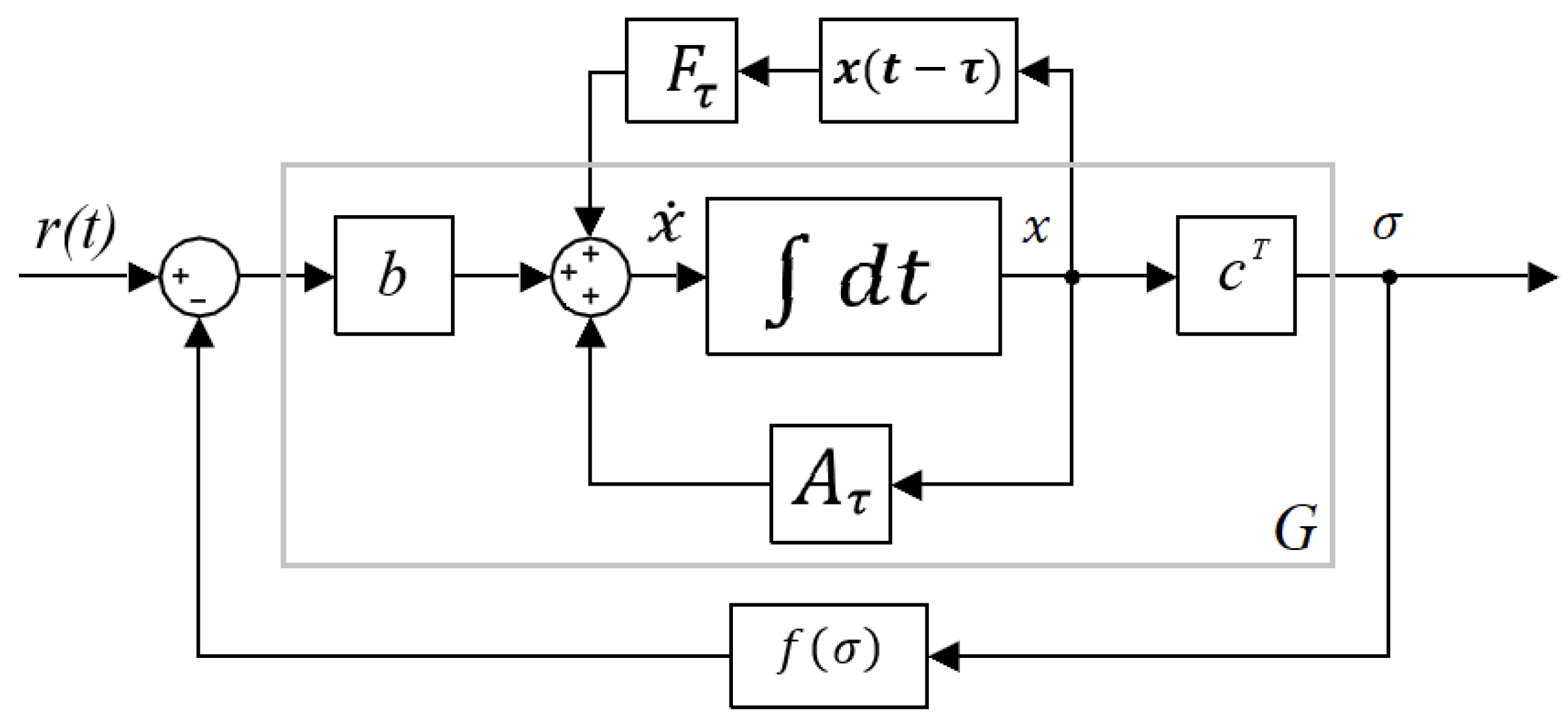
3.1. Lurie Control System
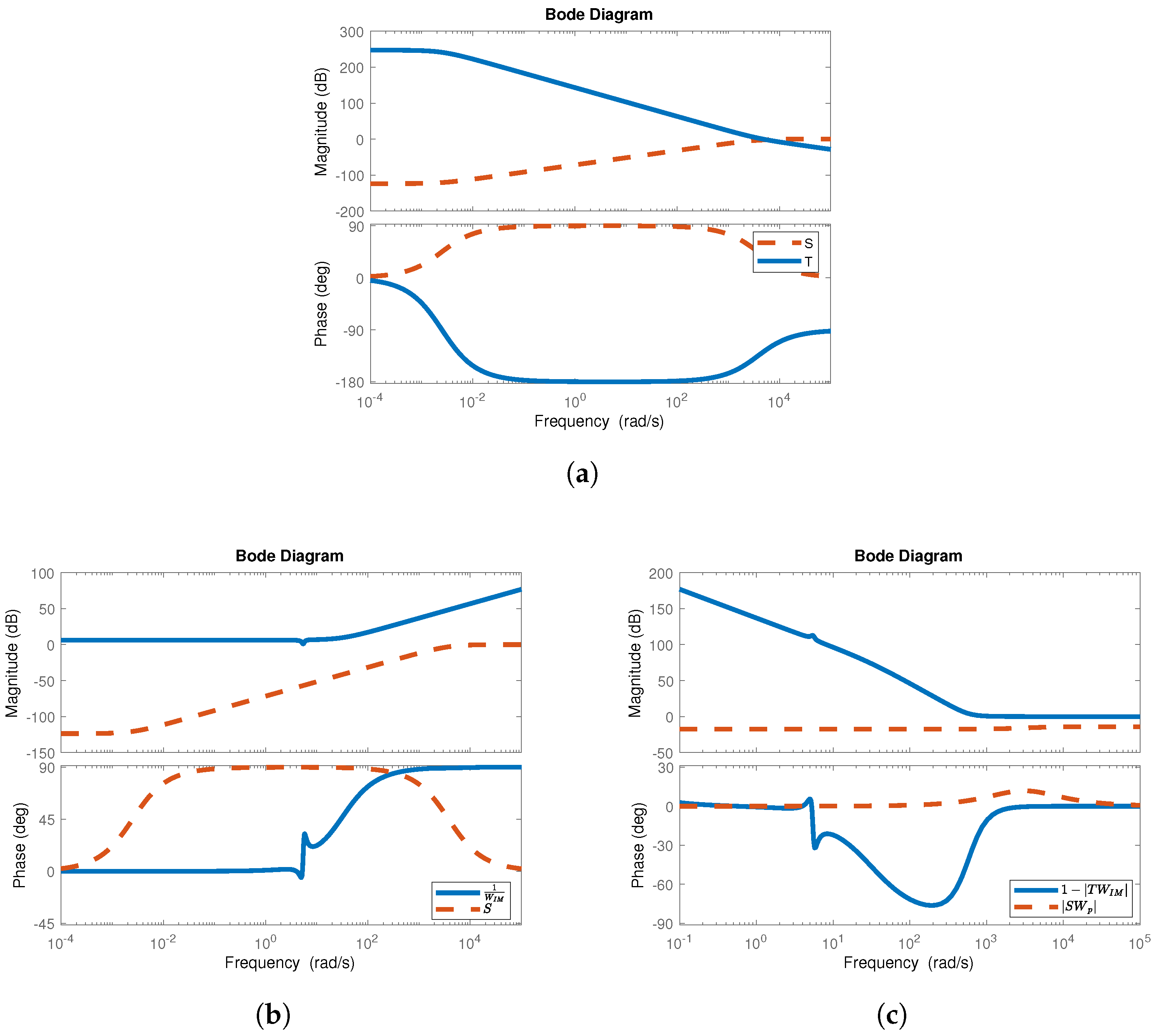
Lurie single-input–single-output (SISO) control systems can be represented by the system in Figure 1a. In this system, there is a linear dynamic represented by system G, and the function f ( σ ) represents a nonlinearity (Figure 1b).
Assuming r 1 = 0 , the system depicted in Figure 1a can be represented by the following set of ordinary differential equations (ODEs):
    x ˙ = A x b f ( σ ) ,     σ = c T x ,
where x R n is the state vector, b , c R n , A R n × n are fixed matrices, and σ f ( σ ) > 0 . In general, the nonlinearity f ( σ ) is a continuous function constrained to the first and third quadrants of the plane (see Figure 1b). It belongs to one of the following families:
F ( 0 , k ] : = { f | f ( 0 ) = 0 , 0 < σ f ( σ ) k σ 2 , σ 0 } ,
F ( 0 , k ) : = { f | f ( 0 ) = 0 , 0 < σ f ( σ ) < k σ 2 , σ 0 } ,
F [ k 1 , k 2 ] : = { f | f ( 0 ) = 0 , k 1 σ 2 σ f ( σ ) k 2 σ 2 , σ 0 } ,
F : = { f | f ( 0 ) = 0 , σ f ( σ ) > 0 , σ 0 } .
A Lurie control system with delay can be described by the block diagram in Figure 2 and corresponding Equation (9):
    x ˙ = A τ x b f ( σ ) + F τ x ( t τ ) + b r 1     σ = c T x .
Here, x R n represents the state vector, τ > 0 denotes a constant real delay, f ( σ ) R , and σ R . The system includes fixed matrices F τ R n × n , b R n , c R n , and A τ R n × n , where A τ is a Hurwitz matrix. Equation (9) is an extension of Equation (4), which includes the time delay.
Figure 2. Block diagrams of the SISO Lurie control system with delay.
Eng 06 00089 g002
The stability analysis of Lurie-type systems has become known in the literature as the study of absolute stability, whose definition is presented below.
Definition 1.
 (Absolute Stability) Assuming null input ( r 1 = 0 ), it is said that system (9) (or system (4)) is absolutely stable if the zero solution of (9) (or system (4)) is globally asymptotically stable in the Lyapunov sense for f ( σ ) F ( 0 , k ] , that is, ϵ > 0 ,   δ ( ϵ ) > 0 , such that the solution x ( t ) : = x ( t , t 0 , x 0 ) of the initial value problem associated to (9) (or system (4)) is unique and satisfies:
x ( t ) < ϵ , t t 0 , i f x 0 < δ ( ϵ ) ,
and for any x 0 R n :
lim t x ( t ) = 0 .
Now, to correlate the Chua circuits of Equations (1) and (3), with the Lurie control systems of Equations (4) and (9), take the nonlinearity as F [ k 1 , k 2 ] , where k 1 = m 0 and k 2 = m 1 , and the matrices as:
A = α α 0 1 1 1 0 β β ρ , b = α 0 0 , c = 1 0 0 , A τ = α α 0 0 1 1 0 β β ρ ,
a n d F τ = 0 0 0 θ 0 0 0 0 0 .

3.2. H Mixed-Sensitivity for Lurie Control Systems

In this subsection, the H mixed-sensitivity (S/KS/T) control theory for Lurie control systems developed by [18] is presented. Firstly, the nonlinearity f in Figure 1b and Equation (4) is modeled as a parametric uncertainty, resulting in a family of plants, G a . By substituting f with a, the perturbed transfer function, G a , is defined as follows:
G a ( s ) = G ( s ) 1 + a G ( s ) ,
where G ( s ) = c T ( s I A ) 1 b represents the transfer function for the linear component shown in Figure 1a and Equation (4). Figure 3 shows the block diagram formats in which Lurie-type systems need to be placed in order for the controller to be developed. The mixed sensitivity method consists of obtaining a controller, K ( s ) , with robust stability and performance by satisfying the following condition [25]:
| | N | | H = m a x ω γ ( N ( j ω ) ) < 1 ,
here, γ serves as an upper bound for the norm, utilized to quantify the size of the matrix N across all frequencies. In the case of SISO systems, N becomes a vector, and γ ( N ) corresponds to the standard Euclidean norm of the vector:
γ ( N ) = | W p S | 2 + | W I M T | 2 + | W u K S | 2 .
In N, such that N = [ W p S W u K S W I M T ] T , one defines the sensitivity function S = ( I + G o K ) 1 and the complementary sensitivity function T = ( I + G o K ) 1 G o K , where G o and K are as shown in Figure 3a and Figure 3b, respectively. The objective is to develop controllers that ensure the system’s stability and performance robustness, as depicted in Figure 3c. The term K S represents the control effort, defined as the product of the controller transfer function, K, and the sensitivity function, S, reflecting the controller’s response to disturbances and noise. Here the perturbed transfer function is represented by G p ( s ) , which is according to (15) and Figure 3a.
G p ( s ) = G o ( s ) 1 + W I M ( s ) δ , | δ | 1 .
The δ -uncertainty is obtained from a of (12), and W p , W u , and W I M are weight functions. The weight W I M is used for modeling the uncertainty and is defined by the uncertainty model of the plant family. Ref. [18] shows in detail how to obtain W I M for a Lurie-type system. The designer selects the weights W u and W p to represent the desired specifications for the closed-loop system. The weight W u is applied to penalize excessive control efforts. According to [25], the W p could be chosen as:
W p = s / M + w b s + w b E ,
where:
M: robustness margin (or robustness parameter), which defines an upper limit for the sensitivity function, balancing performance and robustness. Typically, M > 1 .
w b : bandwidth crossover frequency, which determines the frequency at which the sensitivity function is approximately 1. It is related to system performance in terms of response speed.
E: defines error attenuation at low frequencies and the transition to high frequencies, adjusting the decay rate of the weight W p .
The new nominal model of the plant is represented by G o ( s ) . The functions W I M and G o depend on G (this is shown in Theorems 1 and 3).
For the robustness analysis of stability (RS) and performance (RP), according to [13,25], the conditions are as follows:
R S | S | < 1 | W I M | , ω ;
and
R P | W p S | < 1 | W I M T | , ω .
Figure 3. Block diagrams of the theory of robust control for analysis and synthesis via H mixed-sensitivity. (a) Perturbed transfer function inverse multiplicative. (b) System L p = G p K in closed loop. (c) Complete diagram with all weights.
Eng 06 00089 g003
The following theorem, derived from H mixed-sensitivity techniques, can be used to synthesize controllers for Lurie-type systems without delay (Equation (4)).
Theorem 1.
Given a controller, K ( s ) , and [ k 1 , k 2 ] , the sector that includes f F [ k 1 , k 2 ] (f is replaced by a such that k 1 a k 2 ), then system (4) with a feedback loop containing the controller, K ( s ) , is robustly stable and has a robust performance, if and only if:
W p S W u K ( s ) S W I M k T H < 1 ,
where:
S = ( 1 + G o k ( s ) K ( s ) ) 1 ,
T = ( 1 + G o k ( s ) K ( s ) ) 1 G o k ( s ) K ( s ) ,
W I M k ( s ) = G o k ( s ) ( k 2 + k 1 2 ) ,
with:
G o k ( s ) = G ( s ) 1 + G ( s ) ( k 2 + k 1 2 ) ,
and
G ( s ) = c T ( s I A ) 1 b .
Here, W p and W u are chosen to match specification (19).
Proof. 
The complete proof can be found in Theorems 5 and 6 of the paper [18]. □
Remark 1.
It is important to note that the controller ensures RS and RP when varying the parameter “a”, which varies from k 1 to k 2 and replaces the nonlinearity f. Thus, this theorem proposes a robust control approach to solve a nonlinear control problem. The same observation also applies to Theorem 3.

3.3. Padé Approximations

In this work, Padé’s approximation is used instead of the time delay. Some Padé approximations represented here by [ M / L ] are shown in Table 1. The following theorem presents an important result of the convergence of Padé approximations, which will be used to demonstrate the main result of this paper.
Theorem 2.
Let f ( s ) be a meromorphic function. Suppose that ϵ and δ are given positive numbers. Then M 0 exists such that any Padé approximation [ M / M ] satisfies:
f ( s ) [ M / M ] < ϵ ,
for all M > M 0 on any compact set of s-plane except for a set E M of measure less than δ.
Proof. 
See [37]. □
It is important to note that this convergence is uniform because neither δ nor ϵ depend on s.

4. Main Results

This section presents a new theorem for synthesizing robust controllers for time-delayed Lurie SISO control systems with nonlinearities of type F [ k 1 , k 2 ] . This theorem is directly applicable to Chua systems, since these are a particular case of a Lurie control system, as demonstrated in Section 3.1. Thus, in the following, the newly proposed theorem is employed in designing a robust controller for the modified chaotic Chua circuit, free of delays, as described by [6], which models the dynamics between HR, SNA, and BP in “V-trough” events, which may be a precursor of fatal cardiac events. Next, the same Chua circuit, with an inserted delay, is analyzed and a controller is developed based on the new theory.

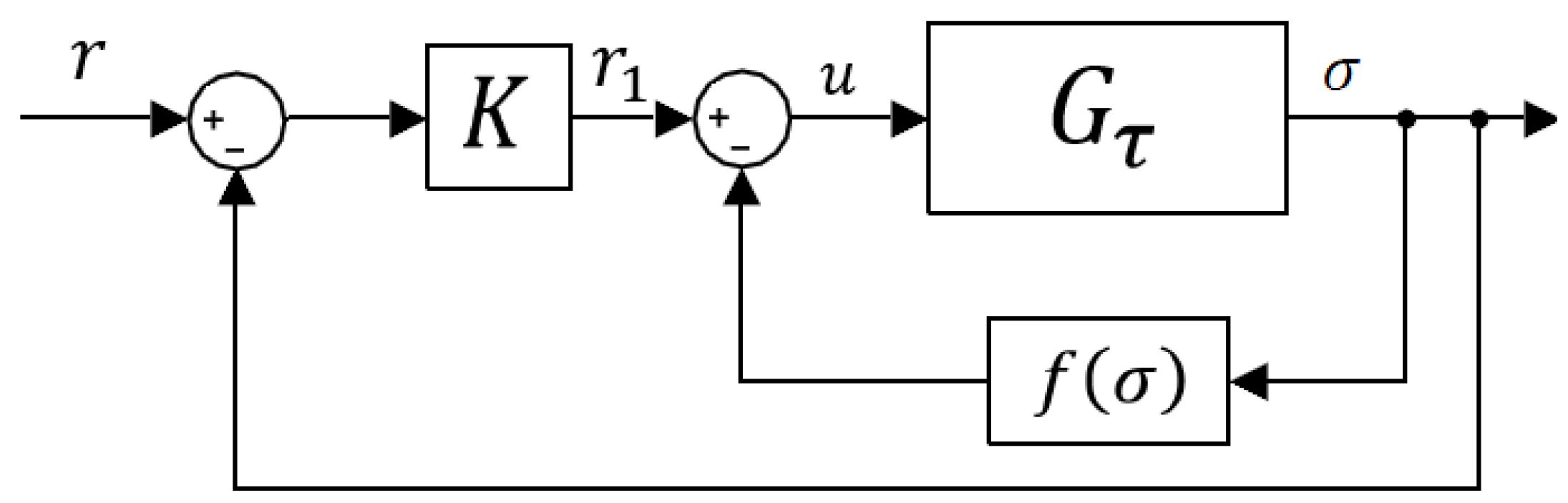
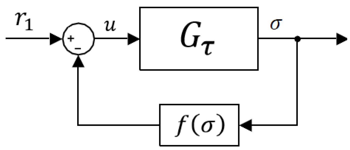
4.1. Theorem for the Synthesis of Lurie SISO Control Systems with Delay

Theorem 3.
Given a controller, K ( s ) , and [ k 1 , k 2 ] , the sector that includes f F [ k 1 , k 2 ] (f is replaced by a such that k 1 a k 2 ), then system (9) with a feedback loop containing the controller, K ( s ) , (Figure 4) is robustly stable and has a robust performance, if and only if:
W p τ S τ , k W u τ K ( s ) S τ , k W I M τ , k T τ , k H < 1 ,
where:
S τ , k = ( 1 + G o τ , k ( s ) K ( s ) ) 1 ,
T τ , k = ( 1 + G o τ , k ( s ) K ( s ) ) 1 G o τ , k ( s ) K ( s ) ,
W I M τ , k ( s ) = G o τ , k ( s ) ( k 2 + k 1 2 ) ,
with:
G o τ , k ( s ) = G τ , k 1 + G τ , k ( k 2 + k 1 2 ) ,
and
G τ , k ( s ) = c T ( s I A τ F τ [ k / k ] ) 1 b .
Here, [ k / k ] represents the Padé approximation, where both the numerator and denominator have a degree of k, and W p τ and W u τ are chosen to match specification (26).
Figure 4. Lurie control system with delay and a feedback loop containing a controller.
Eng 06 00089 g004
Proof. 
Consider initially the system of Figure 2 and Equation (9) placed in the following form:
The equation for the system of Figure 5, for r 1 = 0 , is:
  x ˙ = A τ x + b u + F τ x ( t τ )   σ = c T x .
To obtain G τ ( s ) , as in Figure 5, one must take the transfer function applying the Laplace transform to Equation (32), which relates the input signal, u, to the output signal, σ :
s X ( s ) = A τ X ( s ) + b U ( s ) + F τ e τ s ,
X ( s ) ( s I A τ F τ e τ s ) = b U ( s ) ,
X ( s ) U ( s ) = ( s I A τ F τ e τ s ) 1 b .
But,
σ ( s ) = c T X ( s ) ,
so:
σ ( s ) U ( s ) = c T ( s I A τ F τ e τ s ) 1 b = G τ ( s ) .
When replacing the exponential term with the Padé approximation, it becomes necessary to verify whether the sequence G τ , k converges to G τ . To do so, we define the function ϕ ( s ) = s I A τ F τ e s t and the sequence of functions ϕ k ( s ) = s I A τ F τ [ k / k ] . Every element of F τ [ k / k ] is expressed as a rational function. By Theorem 2, this sequence converges uniformly, and thus the matrix sequence is convergent F τ e s τ . Since s I A can be thought as a constant sequence (which always converges), and since the sum of two convergent sequences of complex matrices also converges, it follows that ϕ k ( s ) converges to ϕ ( s ) . Therefore, this sequence of rational function matrices converges point-to-point. One knows from Theorem 2 that the sequence of Padé’s approximations [ k / k ] converges uniformly to e τ s . The sequence F τ [ k / k ] is composed of elements that demonstrate uniform convergence. Using the -norm ( A = max i ( j | a i j | ) ), which is distinct from the H norm applied in H control, it follows:
ϕ k ( s ) ϕ ( s ) = s I A τ F τ [ k / k ] s I + A τ + F τ e τ s = F τ ( e τ s [ k / k ] ) = max i ( j | [ F τ ] i j | | [ k / k ] e τ s | ) = F τ | e τ s [ k / k ] | .
Since for every ϵ > 0 there exists K > 0 , such that, for all k > K , | [ k / k ] e τ s | < ϵ , one can always choose a ϵ 2 > 0 , such that there is a ϵ = ϵ 2 / F τ , such that there is a K > 0 , such that all k > K . Then, one has:
ϕ k ( s ) ϕ ( s ) = F τ ϵ < ϵ 2 ,
as a result, ϕ k ( s ) converges uniformly under the norm in question. Since the space of matrices is finite-dimensional, convergence in one norm implies convergence in all other norms within the same space. The subsequent step involves establishing the sequence ϕ k 1 ( s ) and determining whether it also converges uniformly. The sequence ϕ k ( s ) exhibits convergence. Moreover, f ( A ) = A 1 is continuous if and only if A G L ( C , n ) , representing the set of n × n complex matrices with a nonzero determinant. In other words, within an open set where f remains continuous, we exclude the finite set of poles where ϕ k ( s ) lacks definition. Since the elements of the matrices ϕ k ( s ) are meromorphic, the set of points where they are not defined has measure zero in C. Therefore, each ϕ k ( s ) is defined almost everywhere in C, meaning it is defined in an open set. It is clear that the function f is defined within this open set and is continuous, then { ϕ k 1 ( s ) } converges in this set point-to-point. It is necessary to demonstrate that, for every ϵ 2 > 0 , there exists a K > 0 , such that for all k > K we have | ϕ k 1 ( s ) ϕ 1 ( s ) | < ϵ 2 . By using the identity S 1 T 1 = S 1 ( S T ) T 1 , one has (in the open set described above, that is, almost everywhere):
ϕ k 1 ( s ) ϕ 1 ( s )     ( s I A τ F τ [ k / k ] ) 1 F τ ( [ k / k ] e s τ ) s I A τ F τ e s τ   = | [ k / k ] e s τ |   ( s I A τ F τ [ k / k ] ) 1 F τ ( s I A τ F τ e s τ ) 1 = Γ ( s ) .
Assume s = j ω . Then, there exists a constant Λ > 0 , such that | Γ ( j ω ) | < Λ , which serves as an upper bound for the factors, as shown in Equation (40). Since [ k / k ] uniformly converges to e s τ , for every ϵ > 0 there exists a K, such that for all k > K we have | [ k / k ] e s τ | < ϵ . Consequently, for every ϵ 2 > 0 , there exists a K, such that for k > K the following holds:
ϕ k 1 ( s ) ϕ 1 ( s ) | [ k / k ] e s τ | Λ < ϵ Λ = ϵ 2 ,
which concludes uniform convergence. Since ϕ k 1 ( s ) is convergent almost everywhere in C and if it is just multiplied by constants on both sides, then c T { ϕ k 1 ( s ) } b continues to converge. Therefore, it is proven that G τ , k converges to G τ .
Now, let us consider the system in Figure 5 with a feedback branch with a controller according to Figure 4. The system of Figure 4 can be placed in the form of Figure 3a,b, and from (12) we have:
G p ( s ) = G τ ( s ) 1 + a G τ ( s ) ,
since one has f F [ k 1 , k 2 ] then k 1 a k 2 , thus:
a = k 1 + ( k 2 k 1 2 ) + ( k 2 k 1 ) 2 δ = ( k 2 + k 1 2 ) + ( k 2 k 1 ) 2 δ , | δ | 1 .
G p ( s ) = G τ ( s ) 1 + G τ ( s ) ( k 2 + k 1 2 ) + G τ ( s ) ( k 2 k 1 2 ) δ ,
dividing the numerator and denominator by 1 + G τ ( s ) ( k 2 + k 1 2 ) , one has:
G p ( s ) = G τ ( s ) 1 + G τ ( s ) ( k 2 + k 1 2 ) 1 + ( G τ ( s ) ( k 2 k 1 2 ) 1 + G τ ( s ) ( k 2 + k 1 2 ) ) δ ,
so one has inverse multiplicative uncertainty, according to (15): G p ( s ) = G o τ ( s ) 1 + W I M ( s ) δ , | δ | 1 . So:
G o τ ( s ) = G τ ( s ) 1 + G τ ( s ) ( k 2 + k 1 2 ) ,
W I M τ ( s ) = G o τ ( s ) ( k 2 k 1 2 ) ,
S = ( I + G o τ K ) 1 ,
T = ( I + G o τ K ) 1 G o τ K .
It is verified that G τ , k converges to G τ . In addition, it is known that linear operations of convergent sequences also converge, and therefore the result holds for G o , k τ ( s ) , which allows us to derive S τ , k , T τ , k , W I M τ , k , and G o τ , k . The weights W p τ and W u τ must be inserted in order to obtain a system according to Figure 3c. Finally, by condition (13), the theorem is demonstrated. □

4.2. Controller Design and Simulations

The Matlab function m i x s y n ( G , W 1 , W 2 , W 3 ) was used to design the controller. This computes a controller that minimizes the H norm of the weighted closed-loop transfer function, given by N = [ W 1 S W 2 K S W 3 T ] T . Proceeding from Theorem 3, we insert the functions G o τ , k , W p τ , W I M τ , k , and W u τ in place of G, W 1 , W 2 , and W 3 to design the frequency responses for disturbance rejection, tracking, noise reduction, controller effort, and robustness. Therefore, this function calculates a controller, K ( s ) , by solving the problem m i n K | N ( K ) | , while also returning the value of γ (for more information, see Mathworks in [38]). The block diagram analogous to the one used in Simulink is shown in Figure 6.
Remark 2.
In conventional control systems, the equilibrium point is often used as a reference. However, in the context of this study, where we deal with cardiac responses, a sinusoidal reference signal is more appropriate. This choice is justified by the fact that heart rate variability and various physiological dynamics of the cardiovascular system exhibit natural oscillatory behavior. By using a sinusoidal reference, we ensure that the controller’s performance is evaluated under conditions that better reflect the physiological characteristics of the problem, making the analysis more realistic and relevant for medical applications.

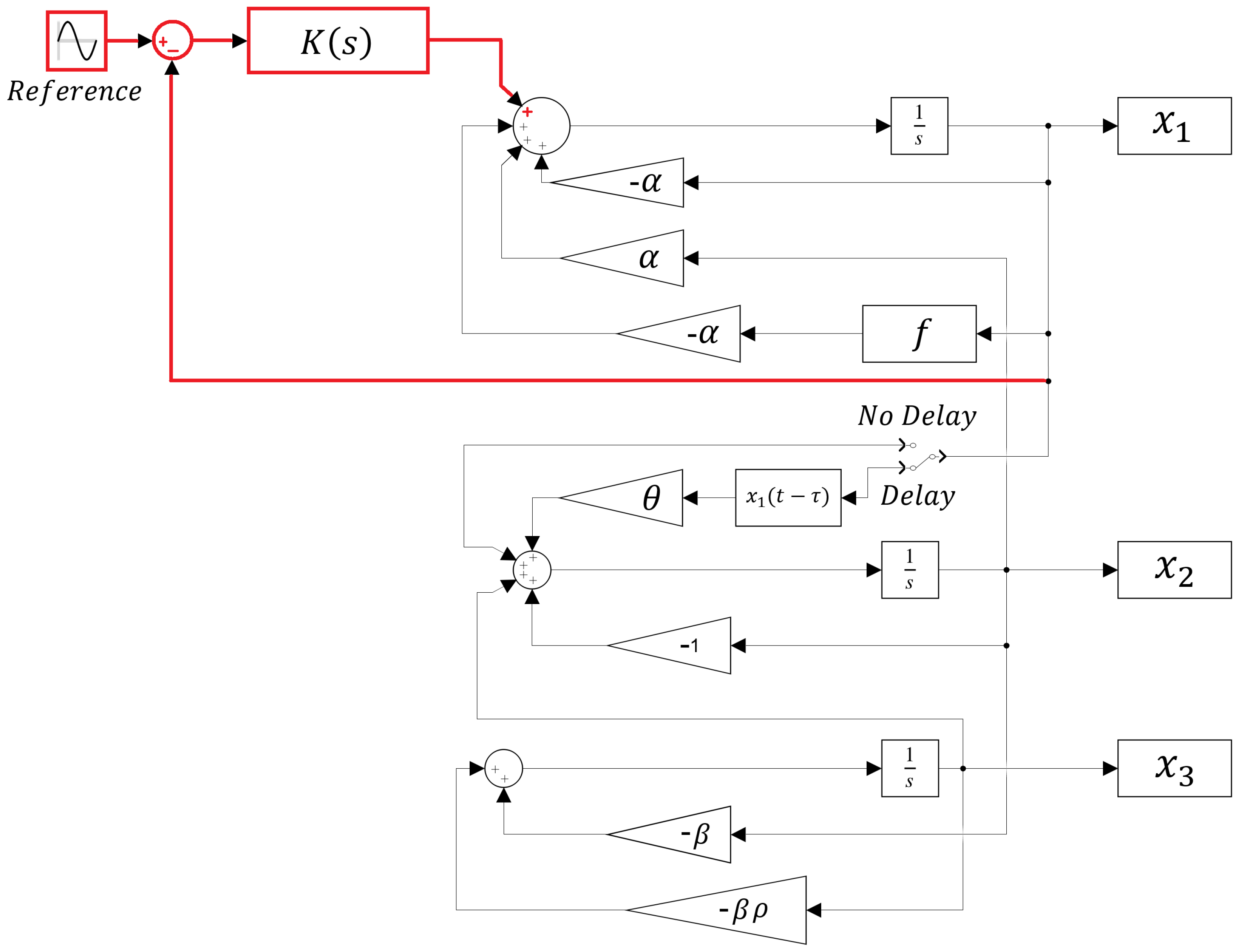
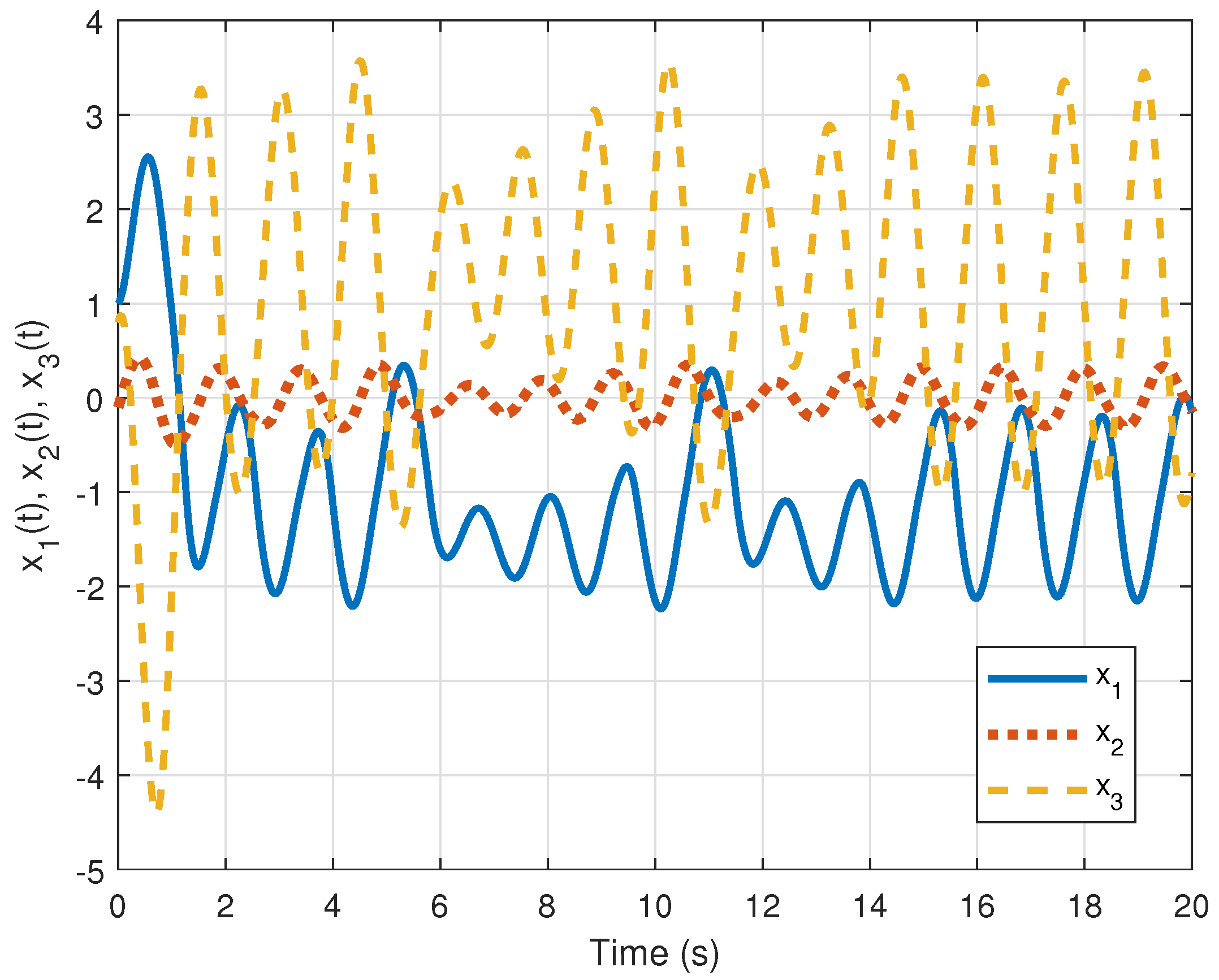
4.2.1. Controller for the Chua Circuit (1) That Models HR, SNA, and BP in the SCD

The parameters for the Chua circuit (1) that models the interaction between HR, SNA, and BP that generates pathological dynamics associated with the V-shaped trough that can lead to sudden cardiac death, according to [6], are α = 15.6 ; β = 30 ; ρ = 0.0025 ; m 0 = 8 / 7 ; and m 1 = 5 / 7 . The simulation of this model is shown in Figure 7.
To design a controller using H mixed-sensitivity (S/KS/T) for (1), the sector is f F [ k 1 , k 2 ] , and thus we adopt k 1 = m 0 . So, by Theorem 3, one has G τ , k ( s ) = c T ( s I A F τ [ k / k ] ) 1 b , with
A = α α 0 1 1 1 0 β β ρ , b = α 0 0 , c = 1 0 0 , a n d F τ = 0 .
Now, by Theorem 3, one has G o τ , k and W I M τ , k . According to (16), W p τ = W p ( s ) = s / M + w b s + w b E and the parameters M = 5 , E = 5 × 10 6 , and w b = 500 are used. E < < 1 was chosen to obtain a small stationary error. M = 5 was chosen, according to the value suggested in [25]. We chose a high value for w b (in a similar way to [39]) to improve the tracking capability for dynamic reference signals (which in this case is a sinusoidal signal). Finally, using the Matlab function m i x s y n ( G o τ , k , W p τ , W I M τ , k , W u τ ) , the controller, K ( s ) , is obtained:
K ( s ) = 243.4 s 6 1.518 e 04 s 5 2.594 e 05 s 4 1.151 e 06 s 3 1.425 e 07 s 2 2.061 e 07 s 1.99 e 08 s 6 + 32.24 s 5 + 110.5 s 4 + 1891 s 3 + 2384 s 2 + 2.718 e 04 s + 67.94
The value of γ = 0.9432 was achieved with W u τ = 0.1 . This particular value for W u was determined after several trials. A time-domain simulation was conducted using nonlinear function (2):
f ( x 1 ( t ) ) = m 1 x 1 ( t ) + 1 2 ( m 0 m 1 ) ( | x 1 ( t ) + 1 |     | x 1 ( t ) 1 | ) .
The controller was inserted as shown in Figure 6 to act on variable x 1 , i.e., HR. Note in Figure 8 that the HR variable is controlled to follow the sinusoidal reference inserted into the control system input.
Furthermore, Figure 9 allows the analysis of robustness in terms of stability and performance of system (1) with the controller (50). Figure 9a presents the Bode diagrams of the sensitivity (S) and complementary sensitivity (T) functions. In Figure 9b, the Bode diagram for stability robustness (RS) analysis is shown, where it is verified that condition (17) is met. Similarly, Figure 9c shows that condition (18) is satisfied, thus ensuring performance robustness (RP).

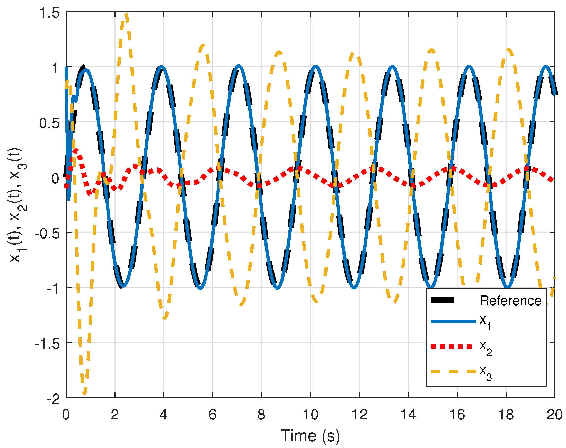
4.2.2. Controller for the Delayed Chua Circuit (3)

The parameters for the Chua circuit (3) that suggests a new model with delay for the interaction between HR, SNA, and BP in SCD are the same for the constants α , β , ρ , m 0 , and m 1 , and for the matrices b and c. As we now have the case of delay, the parameters τ = 5 and θ = 0.5 and the matrices A τ and F τ are included:
A τ = α α 0 0 1 1 0 β β ρ , a n d F τ = 0 0 0 θ 0 0 0 0 0 .
Figure 10 shows the time response of a simulation of the Chua circuit with delay (3). It is clear to see that the main difference provided by the delay in the comparison between Figure 7 and Figure 10 is an increase in the amplitude of the delayed system. Furthermore, just as Osaka observed in model (1), here too we find that the SNA peaks precede the HR peaks and BP nadirs for the delayed model.
To design a controller using H mixed-sensitivity (S/KS/T) for (3), the same parameters and weight functions are used, with the exception of G τ , k ( s ) = c T ( s I A F τ [ k / k ] k ) 1 b , which changes due to new matrices A τ and F τ . Using the Matlab function m i x s y n ( G o τ , k , W p τ , W I M τ , k , W u τ ) , the controller, K ( s ) , is obtained (we do not present the controller’s transfer function here because it is of high order). The gamma value γ = 0.9432 was reached with W u τ = 0.1 . Again, the controller was inserted according to Figure 6 to act on the variable x 1 , i.e., HR. Note in Figure 11 that the HR variable is controlled following the sinusoidal reference entered at the input of the control system.
As in the previous section, where the system without delay was analyzed, the Bode diagrams of the sensitivity and complementary sensitivity functions are shown below (Figure 12a). In addition, it can be seen that the RS (Figure 12b) and RP (Figure 12c) conditions are satisfied for the control of the Chua circuit with delay.

5. Discussion

The primary objective of this study was to propose a method for developing a controller for the modified Chua circuit presented in [6]. However, after some analysis, it became possible to propose a similar circuit with a delay. This led to the need to devise Theorem 3. This theorem is an extension of Theorem 1, which was already used with delay in [18], although no formal proof had been provided.
The results obtained from the analysis of the modified Chua circuit with delay show that the increase in the amplitude of the responses observed may reflect characteristics of autonomic instability often associated with critical conditions, like arrhythmias and sudden cardiac death. The meaning of the variables x 1 , x 2 , and x 3 in the model is equivalent to heart rate (HR), sympathetic nervous system (SNA) activity, and blood pressure (BP), respectively, with the current inclusion of the delay providing an advance of the theory developed by [6], further contributing as a useful bridge between the mathematical behavior of the circuit and physiological phenomena.
Regarding the impact of delay on performance, it is generally assumed to be a source of performance degradation. However, as reported in [40], appropriate delays can actually enhance system performance. In this work, delay is used to model SCD, aiming to produce an artificial temporal response that most closely resembles a biological one, so that its adjustment (either increasing or decreasing it) can improve the model’s ability to accurately represent a biological system. Furthermore, after implementing control, simulations confirmed that the developed controller maintains its performance regardless of the delay value, validating Theorem 3, whose condition ensures controller robustness. Thus, in the controlled system, performance remains unaffected, as the designed controller satisfies the theorem’s condition, guaranteeing robustness in performance.
This work focuses on the continuous-time case with delay; however, in the discrete domain, future investigations could follow the approach proposed by [41], which addresses the stabilization of Lurie systems using sampled-data control within a hybrid continuous-discrete structure. While the present study applies H control to regulate the dynamics of the Chua circuit for biomedical applications, ref. [41] propose an iterative method (CCLI) to compute discrete controller gains, taking into account delays and data loss. This comparison suggests that discrete-time methods could be adapted to control delayed physiological circuits, especially in implantable devices operating with sampled signals. As future directions, we propose: (i) exploring the application of sampled-data control to biomedical circuits with delays, and (ii) developing hybrid control strategies that combine robust continuous-time techniques with discrete-time structures to achieve higher efficiency in real physiological systems.
As far as controlling the variables is concerned, in this work, as it is a first approach, we opted to control only one variable, HR. However, in the time responses of Figure 8 and Figure 11 it can be seen that, by controlling the HR, the other variables automatically take on new stable behaviors. Further research is needed to develop controllers that also control the other variables. Implementing an external controller that dynamically adjusts the system’s variables in response to dangerous conditions, such as sympathetic dysregulation or BP fluctuations, could provide a more robust means of stabilization. Such a controller could apply corrective stimuli, such as those used in advanced pacemakers or neurostimulation devices, to mitigate chaotic patterns and reduce excessive sympathetic activity.
The practical application of these discoveries could culminate in the development of advanced physical devices that modulate not only the heart rhythm, but also the dynamic interaction between HR, SNA, and BP. Such a device would have a broader approach, continuously adjusting to the patient’s conditions to prevent physiological mismatches. Such technology could prove especially useful in high-risk populations, such as patients with heart failure or uncontrolled hypertension, where autonomic instability is prevalent.
The limitations of this work are that the focus here was not on developing a new model with delay, but on developing a controller. Therefore, further research should be carried out with the new model proposed in this work (the inclusion of the delay). Furthermore, in general, although the modified Chua circuit model offers valuable insights, it represents a simplification of real cardiovascular dynamics. Additional factors, such as the influence of metabolic, hormonal, and mechanical variables, could be integrated into future iterations of the model. In addition, the real-world application of devices utilizing this concept would require substantial refinement, including experimental validation and adaptation to respond to real-time physiological signals.

6. Conclusions

This work presents a new control methodology for delayed Chua circuits, addressing the problem of controlling HR in the Osaka model [6], as well as in the updated delayed model outlined by Equation (3). Furthermore, the developed theory is applicable to other SISO Lurie-type systems with delay. For future work, it is worth considering the development of controllers to manage other variables of the model, namely SNA and BP. Additionally, refinement and validation using real physiological data for the delayed Chua circuit are necessary, as this study primarily focuses on the development of the controller. Future work should incorporate actual physiological data, such as heart rate (HR) and blood pressure (BP), to further verify the feasibility of the model in practical applications, as well as present a detailed analysis of the dynamics of the delayed Chua circuit presented in this work.
Future research should advance the integration of Chua’s circuit into a medical device for blood pressure control. Initially, the goal is to develop an experimental platform with electronic components to implement both Chua’s circuit and the controller. The implementation can be carried out using the Hardware-In-The-Loop (HIL) methodology [42], allowing interaction between analog and computational electronic systems. This approach will contribute to expanding knowledge, reducing costs, and enhancing the scalability of bench experiments, representing an innovative strategy for treating arrhythmias and preventing fatal events.
After conducting hardware experiments and their proper validation, a prototype can be developed for future in vivo experiments. This prototype would integrate advanced detection, dynamic control, and precise stimulation to stabilize heart rhythm, marking a significant step at the intersection of biomedicine and dynamical systems theory.

Author Contributions

Conceptualization, R.F.P.; methodology, R.F.P., D.C., A.A. and R.F.-P.; software, R.F.P. and D.C.; validation, R.F.P.; formal analysis, R.F.P., D.C., A.A. and R.F.-P.; investigation, R.F.P., D.C., A.A. and R.F.-P.; resources, R.F.-P.; writing—original draft preparation, R.F.P.; writing—review and editing, R.F.P., D.C., A.A. and R.F.-P.; supervision, D.C. and R.F.-P.; funding acquisition, R.F.-P. All authors have read and agreed to the published version of the manuscript.

Funding

This work was funded by Portuguese national funds provided by the Portuguese Foundation for Science and Technology (FCT) (FCT-UIDB/05704/2020) and in the scope of the research project 2 ARTs (PTDC/EMD-EMD/6588/2020). R. F. Pinheiro acknowledges FCT for the financial support through the Institutional Scientific Employment Stimulus CEECINST/00060/2021.

Institutional Review Board Statement

Not applicable.

Informed Consent Statement

Not applicable.

Data Availability Statement

No new data were created or analyzed in this study.

Conflicts of Interest

The authors declare no conflicts of interest.

Abbreviations

The following abbreviations are used in this manuscript:
BPBlood pressure
ICDImplantable cardioverter defibrillator
HRHeart rate
ODEOrdinary differential equations
SCDSudden cardiac death
SISOSingle-input–single-output
SNASympathetic nerve activity

References

  1. Zhao, S.; Ching, C.K.; Huang, D.; Liu, Y.B.; Rodriguez-Guerrero, D.A.; Hussin, A. Improve SCA Investigators. Regional disparities and risk factors of mortality among patients at high risk of sudden cardiac death in emerging countries: A nonrandomized controlled trial. BMC Med. 2024, 22, 130. [Google Scholar] [CrossRef] [PubMed]
  2. Zipes, D.P.; Wellens, H.J. Sudden cardiac death. Circulation 1998, 98, 2334–2351. [Google Scholar] [CrossRef] [PubMed]
  3. Zadok, O.I.B.; Agmon, I.N.; Neiman, V.; Eisen, A.; Golovchiner, G.; Bental, T.; Barsheshet, A. Implantable cardioverter defibrillator for the primary prevention of sudden cardiac death among patients with cancer. Am. J. Cardiol. 2023, 191, 32–38. [Google Scholar] [CrossRef]
  4. Cavalcanti, R.; Aboul-Hosn, N.; Morales, G.; Abdel-Latif, A. Implantable cardioverter defibrillator for the primary prevention of sudden cardiac death in patients with nonischemic cardiomyopathy. Angiology 2018, 69, 297–302. [Google Scholar] [CrossRef]
  5. Philippon, F.; Domain, G.; Sarrazin, J.F.; Nault, I.; O’Hara, G.; Champagne, J.; Steinberg, C. Evolution of devices to prevent sudden cardiac death: Contemporary clinical impacts. Can. J. Cardiol. 2022, 38, 515–525. [Google Scholar] [CrossRef]
  6. Osaka, M. A modified chua circuit simulates a v-shaped trough in autonomic activity as a precursor of sudden cardiac death. Int. J. Bifurc. Chaos 2011, 21, 2713–2722. [Google Scholar] [CrossRef]
  7. Vrana, M.; Pokorny, J.; Marcian, P.; Fejfard, Z. Class I and III antiarrhythmic drugs for prevention of sudden cardiac death and management of postmyocardial infarction arrhythmias. A review. Biomed. Pap. Med. Fac. Palacky Univ. Olomouc 2013, 157, 114–124. [Google Scholar] [CrossRef]
  8. Osaka, M. Sudden Cardiac Death from the Perspective of Nonlinear Dynamics. J. Nippon. Med. Sch. 2018, 85, 11–17. [Google Scholar] [CrossRef]
  9. Vaidyanathan, S.; Rasappan, S. Global chaos synchronization of n-scroll Chua circuit and Lur’e system using backstepping control design with recursive feedback. Arab. J. Sci. Eng. 2014, 39, 3351–3364. [Google Scholar] [CrossRef]
  10. Ma, J.; Zhang, H.; Zhang, J.; Wang, L. Event-based predefined-time anti-synchronization for unified chaotic systems and the application to Chua’s circuit. Chaos Solitons Fractals 2024, 188, 115534. [Google Scholar] [CrossRef]
  11. Amiri, S.; Seyed Moosavi, S.M.; Forouzanfar, M.; Aghajari, E. Addressing asymmetric saturation in chaotic Chua’s circuit switched system: A combined adaptive sliding mode strategy. Int. J. Adapt. Control Signal Process. 2024, 38, 968–985. [Google Scholar] [CrossRef]
  12. Xing, X. Fixed-time Lyapunov criteria of stochastic impulsive time-delay systems and its application to synchronization of Chua’s circuit networks. Neurocomputing 2025, 616, 128943. [Google Scholar] [CrossRef]
  13. Pinheiro, R.F.; Colón, D. Controller by H mixed-sensitivity design (S/KS/T) for Lurie type systems. In Proceedings of the 24th ABCM International Congress of Mechanical Engineering, Curitiba, Brazil, 3–8 December 2017. [Google Scholar]
  14. Pinheiro, R.F.; Colón, D.; Reinoso, L.L.R. Relating Lurie’s problem, Hopfield’s network and Alzheimer’s disease. In Congresso Brasileiro de Automática-CBA; Sociedade Brasileira de AUTOMATICA: Campinas, Brazil, 2020; Volume 2, pp. 1–8. [Google Scholar]
  15. Pinheiro, R.F.; Colón, D. On the μ-analysis and synthesis of MIMO Lurie-type systems with application in complex networks. Circuits Syst. Signal Process. 2021, 40, 193–232. [Google Scholar] [CrossRef]
  16. Pinheiro, R.F. The Lurie Problem and Its Relationships with Artificial Neural Networks and Alzheimer-like Disease. Ph.D. Thesis, University of São Paulo, São Paulo, Brazil, 2021. [Google Scholar]
  17. Pinheiro, R.F.; Colón, D. Robust digital controllers via H design for Lurie type systems. J. Appl. Instrum. Control 2022, 10, 9–18. [Google Scholar]
  18. Pinheiro, R.F.; Colón, D. Analysis and synthesis of single-input-single-output Lurie type systems via H mixed-sensitivity. Trans. Inst. Meas. Control 2022, 44, 133–143. [Google Scholar] [CrossRef]
  19. Pinheiro, R.F.; Colón, D.; Fonseca-Pinto, R. An improved Alzheimer-like disease computational model via delayed Hopfield network with Lurie control system for healing. TechRxiv 2023. [Google Scholar] [CrossRef]
  20. Pinheiro, R.F.; Colón, D. On the μ-analysis and synthesis for uncertain time-delay systems with Padé approximations. J. Frankl. Inst. 2024, 361, 106643. [Google Scholar] [CrossRef]
  21. Pinheiro, R.F.; Fonseca-Pinto, R.; Colón, D. A review of the Lurie problem and its applications in the medical and biological fields. AIMS Math. 2024, 9, 32962–32999. [Google Scholar] [CrossRef]
  22. Doyle, J. Analysis of feedback systems with structured uncertainties. IEE Proc. D (Control Theory Appl.) 1982, 129, 242–250. [Google Scholar] [CrossRef]
  23. Doyle, J. Structured uncertainty in control system design. In Proceedings of the 1985 24th IEEE Conference on Decision and Control, Fort Lauderdale, FL, USA, 11–13 December 1985; pp. 260–265. [Google Scholar]
  24. Zhou, K.; Doyle, J.C.; Glover, K. Robust and Optimal Control; Prentice-Hall, Inc.: Upper Saddle River, NJ, USA, 1996. [Google Scholar]
  25. Skogestad, S.; Postlethwaite, I. Multivariable Feedback Control: Analysis and Design, 2nd ed.; John Wiley & Sons: Hoboken, NJ, USA, 2007. [Google Scholar]
  26. Lurie, A.I.; Postnikov, V.N. On the theory of stability of control systems. Prikl. Mat. Mekh. 1944, 8, 246–248. [Google Scholar]
  27. Kazemy, A.; Farrokhi, M. Synchronization of chaotic Lur’e systems with state and transmission line time delay: A linear matrix inequality approach. Trans. Inst. Meas. Control 2017, 39, 1703–1709. [Google Scholar] [CrossRef]
  28. Lin, H.; Wang, C.; Tan, Y. Hidden extreme multistability with hyperchaos and transient chaos in a Hopfield neural network affected by electromagnetic radiation. Nonlinear Dyn. 2020, 99, 2369–2386. [Google Scholar] [CrossRef]
  29. Venkatesh, Y.V. Frequency-domain stability criteria for SISO and MIMO nonlinear feedback systems with constant and variable time-delays. Control Theory Technol. 2016, 14, 347–368. [Google Scholar] [CrossRef]
  30. Abtahi, S.F.; Yazdi, E.A. Robust control synthesis using coefficient diagram method and µ-analysis: An aerospace example. Int. J. Dyn. Control 2019, 7, 595–606. [Google Scholar] [CrossRef]
  31. Lee, C.M.; Juang, J.C. A novel approach to stability analysis of multivariable Lurie systems. In Proceedings of the IEEE International Conference on Mechatronics and Automation, Niagara Falls, ON, Canada, 29 July–1 August 2005; pp. 199–203. [Google Scholar]
  32. Tan, N.; Atherton, D.P. Robustness analysis of control systems with mixed perturbations. Trans. Inst. Meas. Control 2003, 25, 163–184. [Google Scholar] [CrossRef]
  33. Sun, Z. Recent advances on analysis and design of switched linear systems. Control Theory Technol. 2017, 15, 242–244. [Google Scholar] [CrossRef]
  34. Imani, A. A multi-loop switching controller for aircraft gas turbine engine with stability proof. Int. J. Control. Autom. Syst. 2019, 17, 1359–1368. [Google Scholar] [CrossRef]
  35. Duan, W.; Du, B.; Li, Y.; Shen, C.; Zhu, X.; Li, X.; Chen, J. Improved sufficient LMI conditions for the robust stability of time-delayed neutral-type Lur’e systems. Int. J. Control Autom. Syst. 2018, 16, 2343–2353. [Google Scholar] [CrossRef]
  36. Wang, W.; Zeng, H.B. A looped functional method to design state feedback controllers for Lurie networked control systems. IEEE/CAA J. Autom. Sin. 2023, 10, 1093–1095. [Google Scholar] [CrossRef]
  37. Baker, G.; Grave-Morris, P.R. Padé Approximants; Addison-Wesley Publishing Company: Boston, MA, USA, 1981. [Google Scholar]
  38. MathWorks. mixsyn (Robust Control Toolbox). MathWorks. Available online: https://www.mathworks.com/help/robust/ref/dynamicsystem.mixsyn.html (accessed on 19 December 2024).
  39. Koleff, L.; Matakas, L.; Pellini, E. H-infinity current control of the LC coupled voltage source inverter. In Proceedings of the 2017 IEEE Energy Conversion Congress and Exposition (ECCE), Cincinnati, OH, USA, 1–5 October 2017; pp. 5347–5354. [Google Scholar]
  40. Zeng, H.B.; Zhai, Z.L.; He, Y.; Teo, K.L.; Wang, W. New insights on stability of sampled-data systems with time-delay. Appl. Math. Comput. 2020, 374, 125041. [Google Scholar] [CrossRef]
  41. Wang, W.; Liang, J.M.; Zeng, H.B. Sampled-data-based stability and stabilization of Lurie systems. Appl. Math. Comput. 2025, 501, 129455. [Google Scholar] [CrossRef]
  42. Gaspar, J.F.; Pinheiro, R.F.; Mendes, M.J.; Kamarlouei, M.; Soares, C.G. Review on hardware-in-the-loop simulation of wave energy converters and power take-offs. Renew. Sustain. Energy Rev. 2024, 191, 114144. [Google Scholar] [CrossRef]
Figure 1. The Lurie system in SISO case: (a) block diagram of the SISO Lurie control system; (b) types of functions f.
Eng 06 00089 g001
Figure 5. Simplified block diagram for Lurie control system with delay of Figure 2.
Eng 06 00089 g005
Figure 6. Block diagram corresponding to the Chua circuits with the control system. To have simulations of only the Chua circuits without the control system, remove the part highlighted in red (bold). The selector switch (No Delay/Delay) allows us to select the Chua circuit without delay (1) or with delay (3).
Eng 06 00089 g006
Figure 7. Time response for the Chua circuit (1) that models the interaction between HR ( x 1 ), SNA ( x 2 ), and BP ( x 3 ) generating a V-shaped trough. The figure was obtained using Simulink with the block diagram analogous to Figure 6 without the control part (highlighted in red/bold) and with the switch set to “No Delay”.
Eng 06 00089 g007
Figure 8. Time response of the Chua circuit (1) controlled. One has the HR variable ( x 1 ) under control, which follows the sinusoidal input of amplitude 1. The other variables are also altered, acquiring stability. The figure was obtained using Simulink with the block diagram analogous to Figure 6 including the control part (highlighted in red/bold) and with the switch set to “No Delay”.
Eng 06 00089 g008
Figure 9. Analysis of RS and RP for the control of Chua’s circuit without delay. (a) Bode diagram of the functions S and T. (b) Analysis of RS according to condition (17). (c) Analysis of RP according to condition (18).
Eng 06 00089 g009
Figure 10. Time response for the Chua circuit with delay (3). The figure was obtained using Simulink with the block diagram analogous to Figure 6 without the control part (highlighted in red/bold) and with the switch set to “Delay”.
Eng 06 00089 g010
Figure 11. Time response of the controlled Chua circuit (3). The HR variable ( x 1 ) under control follows the sinusoidal input of amplitude 1. The other variables are also altered, acquiring stability. The figure was obtained using Simulink with the block diagram analogous to Figure 6 including the control part (highlighted in red/bold) and with the switch set to “Delay”.
Eng 06 00089 g011
Figure 12. Analysis of RS and RP for the control of Chua’s circuit with delay. (a) Bode diagram of the functions S and T. (b) Analysis of RS according to condition (17). (c) Analysis of RP according to condition (18).
Eng 06 00089 g012
Table 1. Padé table of exp(s).
M / L 012
0 1 1 1 + s 1 2 + 2 s + s 2 2
1 1 1 s 2 + s 2 s 6 + 4 s + s 2 6 2 s
2 2 2 2 s + s 2 6 + 2 s 6 4 s + s 2 12 + 6 s + s 2 12 6 s + s 2
Disclaimer/Publisher’s Note: The statements, opinions and data contained in all publications are solely those of the individual author(s) and contributor(s) and not of MDPI and/or the editor(s). MDPI and/or the editor(s) disclaim responsibility for any injury to people or property resulting from any ideas, methods, instructions or products referred to in the content.

