
Assessing Natural Variation as a Baseline for Biodiversity Monitoring: The Case of an East Mediterranean Canyon

 ,
,
Abstract
:
1. Introduction
2. Materials and Methods
2.1. The Study Area—“Evolution Canyon” II, Lower Nahal Keziv, and Results from the 1998–2000 Period
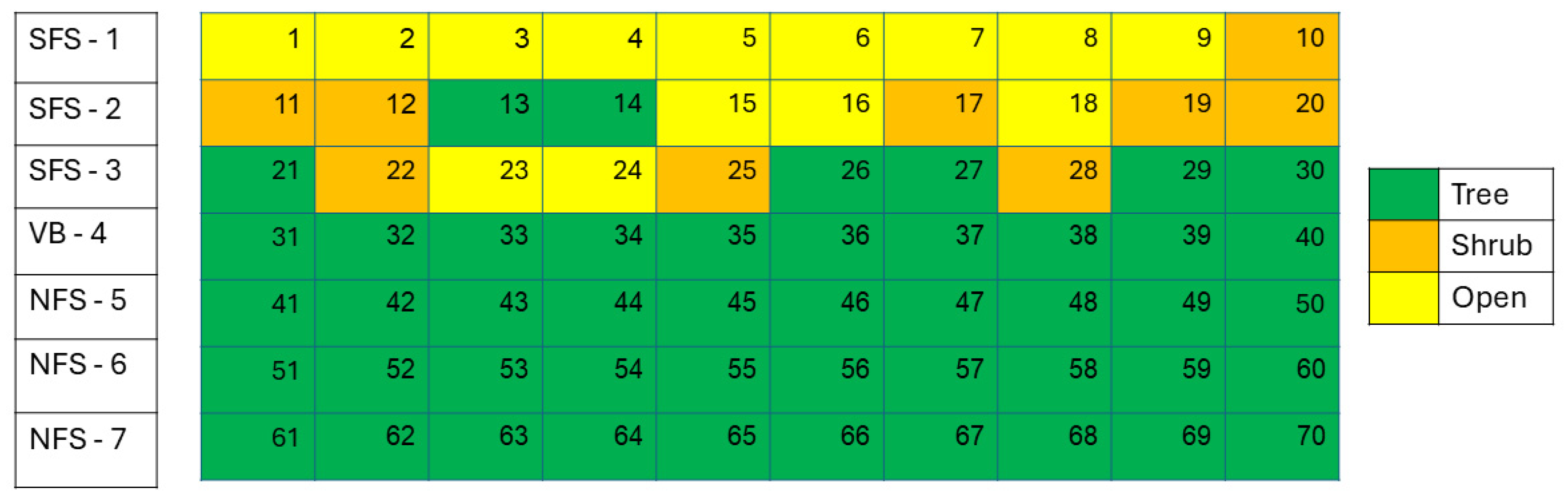
2.2. Topography and Sampling Rows
2.3. Plant Survey and Documentation
2.4. Beetle and Ant Collection and Identification
2.5. Statistical Analysis
2.6. Environmental Changes Between Periods
3. Results
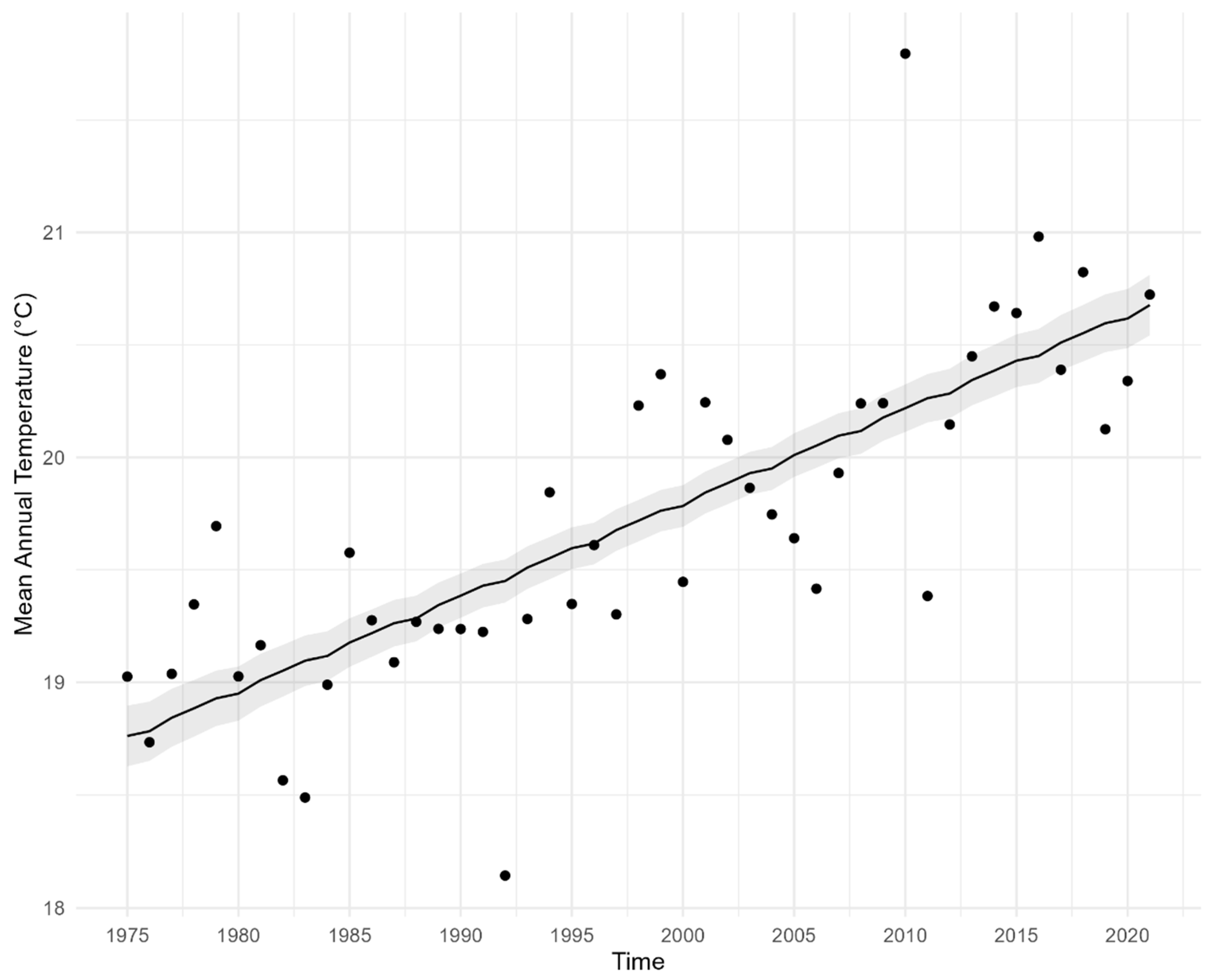
3.1. Climate Measures
3.2. Plants
3.2.1. General Findings
3.2.2. NDVI Results
3.2.3. Detailed Comparison

| Taxon | Research Period | SFS | Overlap Between Slopes | NFS | Species Richness Ratio |
|---|---|---|---|---|---|
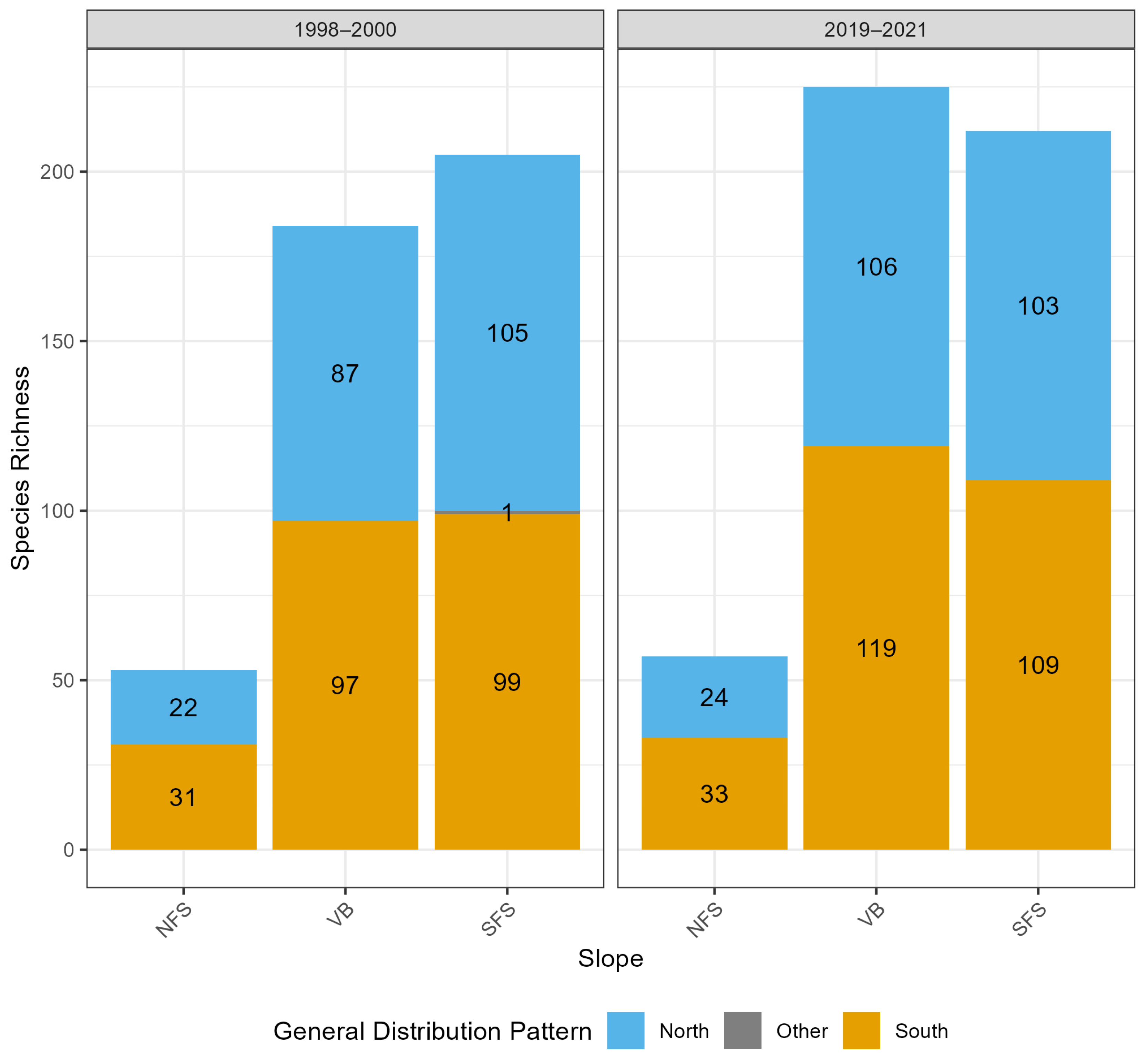
| Plants | 1998–2000 | 205 | 28 (12.2%) | 53 | 3.87 |
| 2019–2021 | 212 | 31 (13%) | 57 | 3.72 | |
| Turnover | 87/252—34.5% | 20/65—30.8% | |||
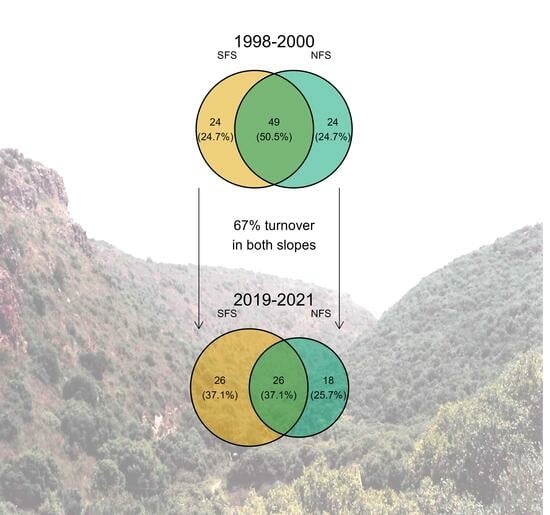
| Beetles (pitfall traps) | 1998–2000 | 73 | 49 (50.5%) | 73 | 1 |
| 2019–2021 | 52 | 26 (37.1%) | 44 | 1.18 | |
| Turnover | 63/94—67% | 59/88—67% | |||
| Beetles (net) | 1998–2000 | 105 | 19 (16.5%) | 29 | 3.62 |
| 2019–2021 | 85 | 13 (12.5%) | 32 | 2.66 | |
| Turnover | 134/162—82.7% | 43/52—82.7% | |||
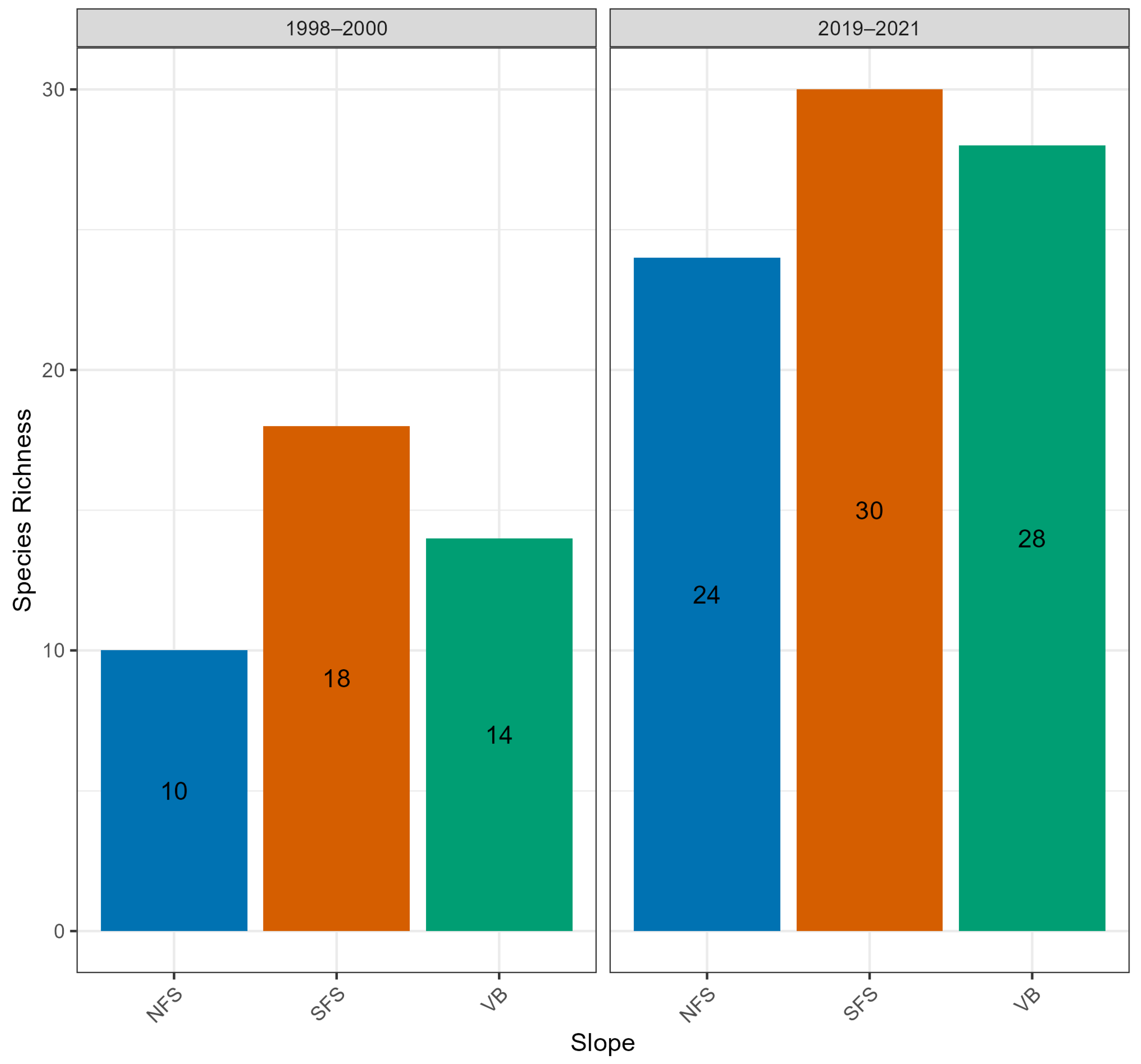
| Ants | 1998–2000 | 18 | 9 (47.4%) | 10 | 1.8 |
| 2019–2021 | 30 | 17 (45.9%) | 24 | 1.25 | |
| Turnover | 20/34—58.8% | 20/27—74.1% |
3.3. Beetles
3.4. Ants
4. Discussion
4.1. Persistence of Inter-Slope Differences Despite a High Species Turnover
4.2. Implications for Monitoring Anthropogenic Effects on Biodiversity
4.2.1. Effects of Rainfall Variation
4.2.2. Effects of Natural Stochastic Dynamics/Autonomous Turnovers
5. Conclusions
Supplementary Materials
Author Contributions
Funding
Data Availability Statement
Acknowledgments
Conflicts of Interest
Appendix A. Extended Methods
Appendix A.1. Definitions of Global Distribution Patterns
Appendix A.2. Beetle Families on Whom the Taxonomic Identification Effort Was Focused (Listed Alphabetically)
Appendix A.3. Extended Descriptions of Methods
Appendix A.4. Statistical Specifications for the Full Models per the Analyzed Index
- Taxa: Plants, beetles (separately for flying and ground-dwelling species) and ants.
- Dependent variable: Species richness per period and line combination.
- Model type: Generalized linear model (GLM).
- Distribution: We used the dispersion parameter to choose between Poisson and negative binomial distributions.
- Predictors: Period (1998–2000 vs. 2019–2021), the slope (north-facing, south-facing or valley bottom) and their interaction.
- Taxon: Plants.
- Dependent variable: Spatial mean of NDVI values from August 15th to September 30th per annum from 1984 (start of data) until 2022 (one year after the end of the second research period).
- Model type: Generalized linear mixed model (GLMM).
- Distribution: Gamma.
- Predictors: Years since 1984 (start of data), the slope (north-facing, south-facing or valley bottom) and their interaction, and the line number in the study site (1 to 7) as a random predictor.
- Dependent variable: Total annual rainfall (mm) from September to August.
- Model type: Generalized linear model (GLM).
- Distribution: Gaussian (normal).
- Predictors: Years since 1950 (start of data)/1995 (a few years before the first research period).
- Dependent variable: No. of days since September 7th (the earliest recorded rainfall event with at least 10 mm, for a rainfall season defined from September to August) until the calendar date of the first/last day of the rainfall season with at least 10 mm of rainfall.
- Model type: Generalized linear model (GLM).
- Distribution: Gaussian (normal).
- Predictors: Years since 1950 (start of data)/1995 (3 years before the first research period).
- Dependent variable: Mean daily temperature (°C).
- Predictors: Years since 1975 (start of data), sine and cosine of the radian distance between the calendar date and June 21st (one and two harmonics—i.e., allowing up to two annual peaks), all interactions between the number of years since 1975 and each trigonometric function (but not between the trigonometric functions themselves).
- Taxon: Ground-dwelling beetles.
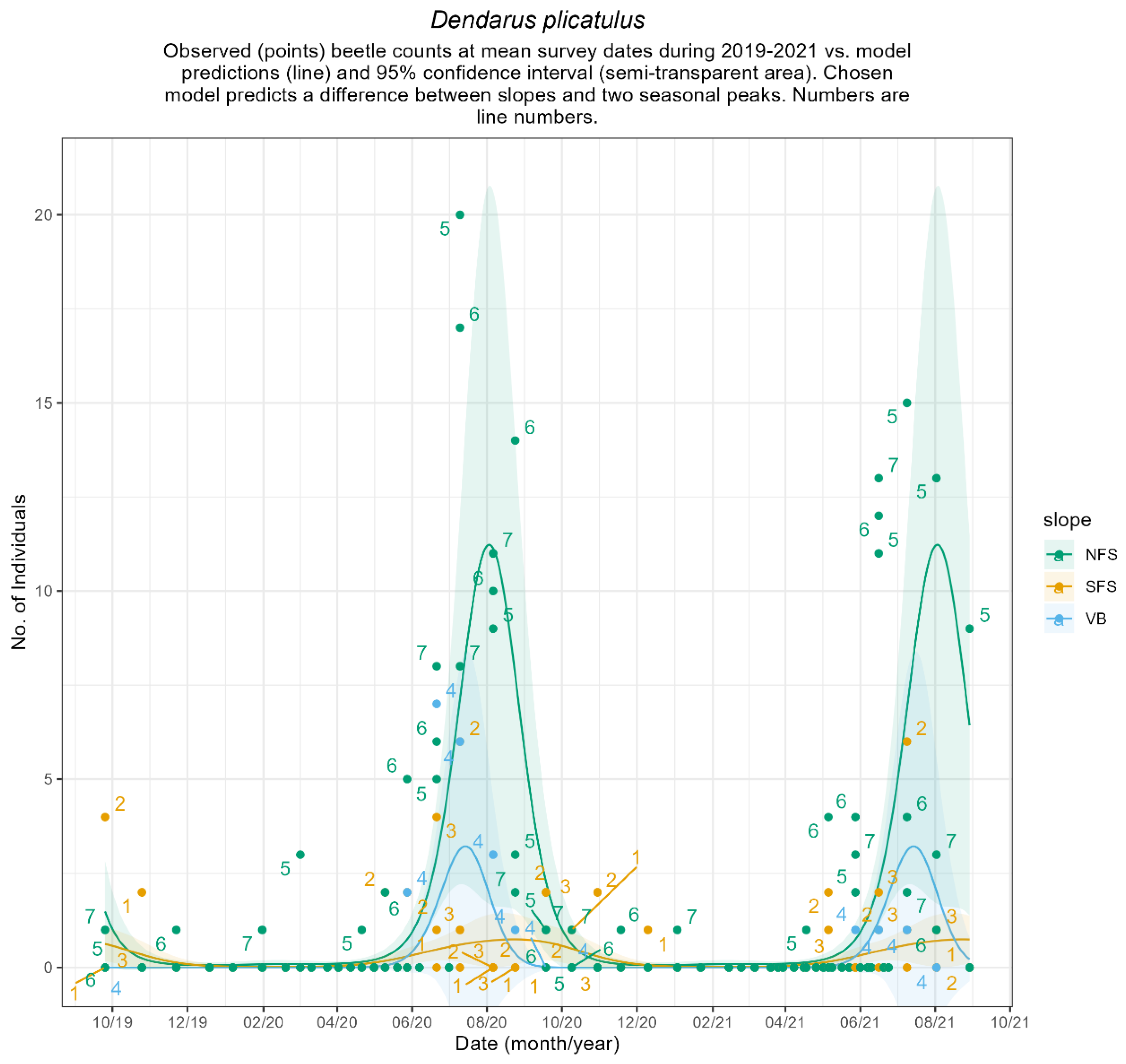
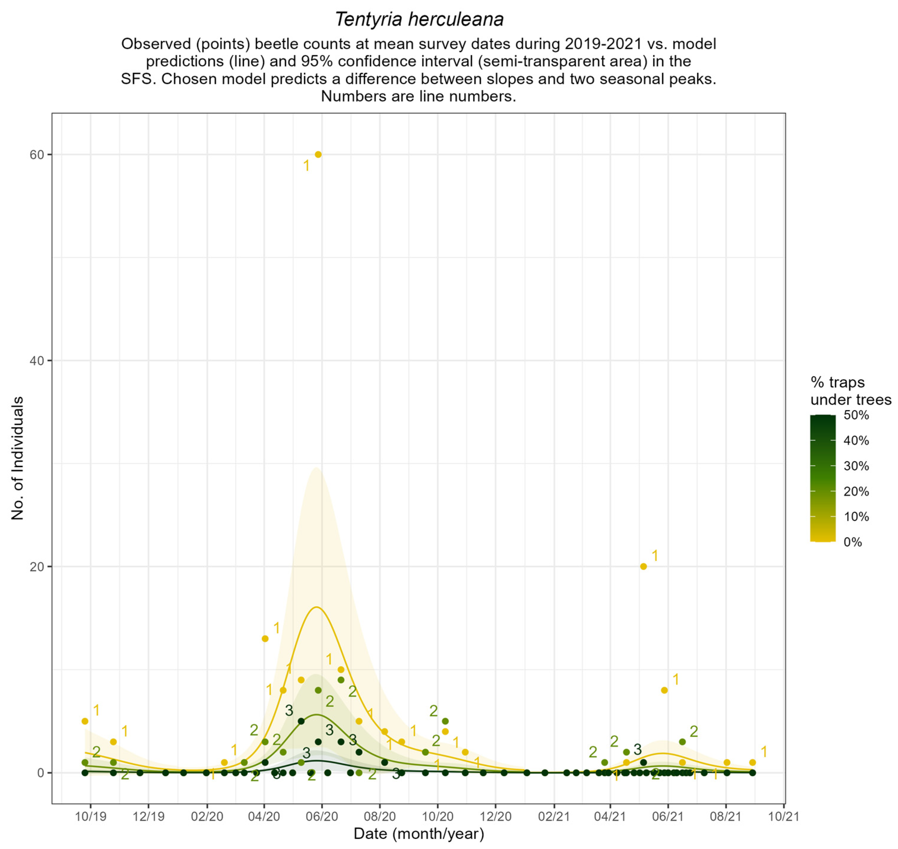
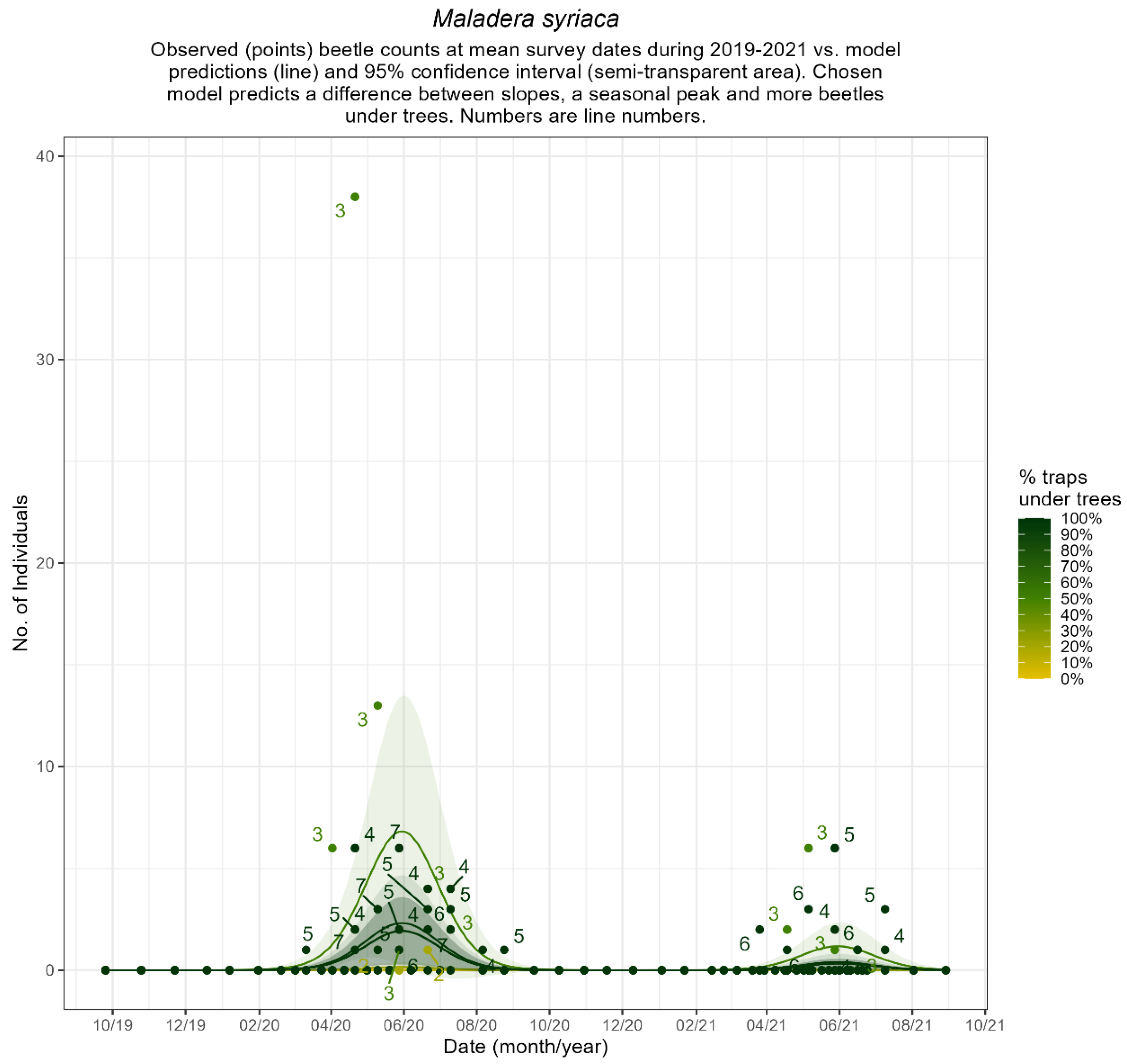
- Dependent variable: Total number of individuals per line of pitfall traps per date during the 2019–2021 research period, analyzed per species, for the 10 most common ground-dwelling beetle species.
- Model type: Cosinor generalized linear mixed model (cosinor GLMM).
- Predictors: Year as a factor (2019, 2020 or 2021), sine and cosine of the radian distance between the calendar date and June 21st (one and two harmonics—i.e., allowing up to two annual peaks), all interactions between the year and each trigonometric function (but not between the trigonometric functions themselves), the slope (north-facing, south-facing or valley bottom), (scaled) percentage of traps beneath the trees per trap line and the trap line number in the study site (1 to 7) as a random predictor.
- Taxon: Ground-dwelling beetles.
- Dependent variable: Total number of individuals per species per line (1 to 7) and period combination. Species with fewer than 10 individuals overall were omitted to avoid spurious results.
- Distribution: We used diagnostic residual plots to choose between Poisson and negative binomial distributions.
- Model type: Generalized linear latent variable model (GLLVM)
- Predictors: Period (1998–2000 vs. 2019–2021), the slope (north-facing, south-facing or valley bottom) and their interaction.
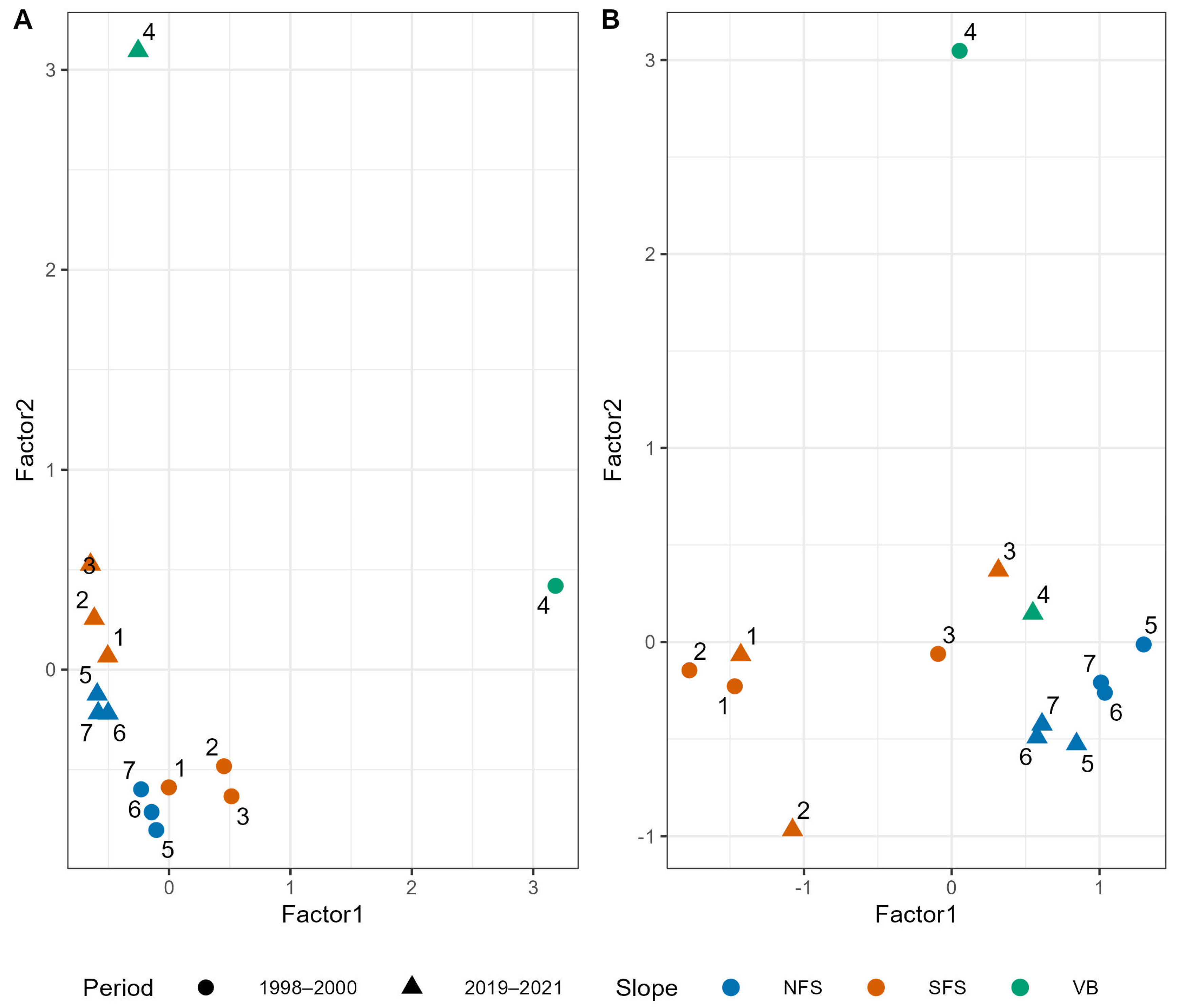
- Taxa: Plants (occurrence), ground-dwelling beetles (abundance), flying and ground-dwelling beetles combined (occurrence) and ants (occurrence).
- Dependent variable: Presence–absence/total number of individuals per species per line (1 to 7) and period combination. When analyzing abundance, species with fewer than 10 individuals overall were omitted to avoid spurious results.
- Distribution: For abundance—negative binomial. For presence–absence—binomial.
- Model type: ecoCopula.
- Predictors: None (unconstrained ordination).
Appendix B. Extended Results
Appendix B.1. Temperature
Appendix B.2. NDVI

Appendix B.3. ecoCopula Results of Net-Collected Beetle Species

Appendix B.4. Seasonal Patterns of Common Ground Beetles


References
- Sánchez-Bayo, F.; Wyckhuys, K.A.G. Worldwide Decline of the Entomofauna: A Review of Its Drivers. Biol. Conserv. 2019, 232, 8–27. [Google Scholar] [CrossRef]
- Didham, R.K.; Basset, Y.; Collins, C.M.; Leather, S.R.; Littlewood, N.A.; Menz, M.H.; Müller, J.; Packer, L.; Saunders, M.E.; Schönrogge, K. Interpreting Insect Declines: Seven Challenges and a Way Forward. Insect Conserv. Divers. 2020, 13, 103–114. [Google Scholar] [CrossRef]
- van Klink, R.; Bowler, D.E.; Gongalsky, K.B.; Swengel, A.B.; Gentile, A.; Chase, J.M. Meta-Analysis Reveals Declines in Terrestrial but Increases in Freshwater Insect Abundances. Science 2020, 368, 417–420. [Google Scholar] [CrossRef] [PubMed]
- Weisser, W.; Blüthgen, N.; Staab, M.; Achury, R.; Müller, J. Experiments Are Needed to Quantify the Main Causes of Insect Decline. Biol. Lett. 2023, 19, 20220500. [Google Scholar] [CrossRef]
- Cardoso, P.; Barton, P.S.; Birkhofer, K.; Chichorro, F.; Deacon, C.; Fartmann, T.; Fukushima, C.S.; Gaigher, R.; Habel, J.C.; Hallmann, C.A. Scientists’ Warning to Humanity on Insect Extinctions. Biol. Conserv. 2020, 242, 108426. [Google Scholar] [CrossRef]
- Wagner, D.L. Insect Declines in the Anthropocene. Annu. Rev. Entomol. 2020, 65, 457–480. [Google Scholar] [CrossRef]
- Wagner, D.L.; Grames, E.M.; Forister, M.L.; Berenbaum, M.R.; Stopak, D. Insect Decline in the Anthropocene: Death by a Thousand Cuts. Proc. Natl. Acad. Sci. USA 2021, 118, e2023989118. [Google Scholar] [CrossRef]
- Rumohr, Q.; Baden, C.U.; Bergtold, M.; Marx, M.T.; Oellers, J.; Schade, M.; Toschki, A.; Maus, C. Drivers and Pressures behind Insect Decline in Central and Western Europe Based on Long-Term Monitoring Data. PLoS ONE 2023, 18, e0289565. [Google Scholar] [CrossRef]
- Harvey, J.A.; Tougeron, K.; Gols, R.; Heinen, R.; Abarca, M.; Abram, P.K.; Basset, Y.; Berg, M.; Boggs, C.; Brodeur, J. Scientists’ Warning on Climate Change and Insects. Ecol. Monogr. 2023, 93, e1553. [Google Scholar] [CrossRef]
- Uhler, J.; Redlich, S.; Zhang, J.; Hothorn, T.; Tobisch, C.; Ewald, J.; Thorn, S.; Seibold, S.; Mitesser, O.; Morinière, J. Relationship of Insect Biomass and Richness with Land Use along a Climate Gradient. Nat. Commun. 2021, 12, 5946. [Google Scholar] [CrossRef]
- Gebert, F.; Bollmann, K.; Schuwirth, N.; Duelli, P.; Weber, D.; Obrist, M.K. Similar Temporal Patterns in Insect Richness, Abundance and Biomass across Major Habitat Types. Insect Conserv. Divers. 2024, 17, 139–154. [Google Scholar] [CrossRef]
- Aronson, J.; Shmida, A. Plant Species Diversity along a Mediterranean-Desert Gradient and Its Correlation with Interannual Rainfall Fluctuations. J. Arid Environ. 1992, 23, 235–247. [Google Scholar] [CrossRef]
- Cowling, R.M.; Samways, M.J. Predicting Global Patterns of Endemic Plant Species Richness. Biodivers. Lett. 1994, 2, 127–131. [Google Scholar] [CrossRef]
- Baselga, A. Determinants of Species Richness, Endemism and Turnover in European Longhorn Beetles. Ecography 2008, 31, 263–271. [Google Scholar] [CrossRef]
- Economo, E.P.; Narula, N.; Friedman, N.R.; Weiser, M.D.; Guénard, B. Macroecology and Macroevolution of the Latitudinal Diversity Gradient in Ants. Nat. Commun. 2018, 9, 1778. [Google Scholar] [CrossRef] [PubMed]
- Heino, J.; Alahuhta, J.; Fattorini, S. Macroecology of Ground Beetles: Species Richness, Range Size and Body Size Show Different Geographical Patterns across a Climatically Heterogeneous Area. J. Biogeogr. 2019, 46, 2548–2557. [Google Scholar] [CrossRef]
- Castro Sánchez-Bermejo, P.; deCastro-Arrazola, I.; Cuesta, E.; Davis, A.L.; Moreno, C.E.; Sánchez-Piñero, F.; Hortal, J. Aridity Drives the Loss of Dung Beetle Taxonomic and Functional Diversity in Three Contrasting Deserts. J. Biogeogr. 2022, 49, 2243–2255. [Google Scholar] [CrossRef]
- Yom-Tov, Y.; Tchernov, E. The Zoogeography of Israel. The Distribution and Abundance at a Zoogeographical Crossroad; Junk, W., Ed.; Springer: Berlin/Heidelberg, Germany, 1988; ISBN 90-6193-650-0. [Google Scholar]
- Biton, L. Israel by the Numbers—Selected Figures from the Annual Statistical Summary of Israel 2023. 2024. Available online: https://www.cbs.gov.il/he/publications/DocLib/isr_in_n/isr_in_n23h.pdf (accessed on 31 January 2025).
- Ben-Moshe, N. State of Nature Report—Israel 2022—Trends and Threats; Hamaarag—Israel’s National Ecosystem Assessment Program, Steinhardt Museum of Natural History, Tel Aviv University: Tel Aviv-Yafo, Israel, 2022; Available online: https://hamaarag.org.il/report/%d7%93%d7%95%d7%97-%d7%9e%d7%a6%d7%91-%d7%94%d7%98%d7%91%d7%a2-2022/ (accessed on 3 March 2025).
- Newbold, T.; Oppenheimer, P.; Etard, A.; Williams, J.J. Tropical and Mediterranean Biodiversity Is Disproportionately Sensitive to Land-Use and Climate Change. Nat. Ecol. Evol. 2020, 4, 1630–1638. [Google Scholar] [CrossRef]
- Zittis, G.; Almazroui, M.; Alpert, P.; Ciais, P.; Cramer, W.; Dahdal, Y.; Fnais, M.; Francis, D.; Hadjinicolaou, P.; Howari, F. Climate Change and Weather Extremes in the Eastern Mediterranean and Middle East. Rev. Geophys. 2022, 60, e2021RG000762. [Google Scholar] [CrossRef]
- Finkel, M.; Ben-Asher, A.; Shmula, G.; Armiach Steinpress, I.; Ganem, Z.; Hammouri, R.; Garcia, E.; Szűts, T.; Gavish-Regev, E. Arachnid Assemblage Composition Diverge between South-and North-Facing Slopes in a Levantine Microgeographic Site. Diversity 2024, 16, 540. [Google Scholar] [CrossRef]
- Liang, J.; Crowther, T.W.; Picard, N.; Wiser, S.; Zhou, M.; Alberti, G.; Schulze, E.-D.; McGuire, A.D.; Bozzato, F.; Pretzsch, H. Positive Biodiversity-Productivity Relationship Predominant in Global Forests. Science 2016, 354, aaf8957. [Google Scholar] [CrossRef] [PubMed]
- Dornelas, M.; Antao, L.H.; Moyes, F.; Bates, A.E.; Magurran, A.E.; Adam, D.; Akhmetzhanova, A.A.; Appeltans, W.; Arcos, J.M.; Arnold, H. BioTIME: A Database of Biodiversity Time Series for the Anthropocene. Glob. Ecol. Biogeogr. 2018, 27, 760–786. [Google Scholar] [CrossRef] [PubMed]
- van Klink, R.; Bowler, D.E.; Comay, O.; Driessen, M.M.; Ernest, S.M.; Gentile, A.; Gilbert, F.; Gongalsky, K.B.; Owen, J.; Pe’er, G. InsectChange: A Global Database of Temporal Changes in Insect and Arachnid Assemblages. Ecology 2021, 102, e03354. [Google Scholar] [CrossRef] [PubMed]
- Comay, O.; Ben Yehuda, O.; Benyamini, D.; Schwartz-Tzachor, R.; Pe’er, I.; Melochna, T.; Pe’er, G. Analysis of Monitoring Data Where Butterflies Fly Year-round. Ecol. Appl. 2020, 30, e02196. [Google Scholar] [CrossRef]
- Nevo, E. Evolution in Action across Life at “Evolution Canyons”, Israel. Trends Evol. Biol. 2009, 1, e3. [Google Scholar] [CrossRef]
- Nevo, E. “Evolution Canyon,” a Potential Microscale Monitor of Global Warming across Life. Proc. Natl. Acad. Sci. USA 2012, 109, 2960–2965. [Google Scholar] [CrossRef]
- Nevo, E. Asian, African and European Biota Meet at ‘Evolution Canyon’ Israel: Local Tests of Global Biodiversity and Genetic Diversity Patterns. Proc. R. Soc. Lond. Ser. B Biol. Sci. 1995, 262, 149–155. [Google Scholar]
- Nevo, E. Evolution in Action across Phylogeny Caused by Microclimatic Stresses at “Evolution Canyon”. Theor. Popul. Biol. 1997, 52, 231–243. [Google Scholar] [CrossRef]
- Nevo, E. Evolution of Genome–Phenome Diversity under Environmental Stress. Proc. Natl. Acad. Sci. USA 2001, 98, 6233–6240. [Google Scholar] [CrossRef]
- Shavit, A.; Griesemer, J. There and Back Again, or the Problem of Locality in Biodiversity Surveys. Philos. Sci. 2009, 76, 273–294. [Google Scholar] [CrossRef]
- Sneh, A.; Bartov, Y.; Rosensaft, M.; Weissbrod, T. Geological Map of Israel 1:200,000; Geological Survey of Israel: Jerusalem, Israel, 1998.
- Shreve, F. Conditions Indirectly Affecting Vertical Distribution on Desert Mountains. Ecology 1922, 3, 269–274. [Google Scholar] [CrossRef]
- Cottle, H.J. Vegetation on North and South Slopes of Mountains in South-Western Texas. Ecology 1932, 13, 121–134. [Google Scholar] [CrossRef]
- Stephenson, S.L. Exposure-Induced Differences in the Vegetation, Soils, and Microclimate of North-and South-Facing Slopes in Southwestern Virginia. Va. J. Sci. 1982, 33, 35–36. [Google Scholar]
- Grishkan, I.; Nevo, E.; Wasser, S.P.; Beharav, A. Adaptive Spatiotemporal Distribution of Soil Microfungi in ‘Evolution Canyon’ II, Lower Nahal Keziv, Western Upper Galilee, Israel. Biol. J. Linn. Soc. 2003, 78, 527–539. [Google Scholar] [CrossRef]
- Van Valen, L. Morphological Variation and Width of Ecological Niche. Am. Nat. 1965, 99, 377–390. [Google Scholar] [CrossRef]
- NOAA El Niño/Southern Oscillation (ENSO). Historical El Nino/La Nina Episodes (1950-Present). In Cold & Warm Episodes by Season; National Oceanic and Atmospheric Administration: Silver Spring, MD, USA, 2017. Available online: https://origin.cpc.ncep.noaa.gov/products/analysis_monitoring/ensostuff/ONI_v5.php (accessed on 3 March 2025).
- Finkel, M.; Fragman, O.; Nevo, E. Biodiversity and Interslope Divergence of Vascular Plants Caused by Sharp Microclimatic Differences at “Evolution Canyon II”, Lower Nahal Keziv, Upper Galilee, Israel. Isr. J. Plant Sci. 2001, 49, 285–296. [Google Scholar] [CrossRef]
- Finkel, M.; Chikatunov, V.I.; Nevo, E. Coleoptera of “Evolution Canyon” II: Lower Nahal Keziv, Western Upper Galilee, Israel; Pensoft Publishers: Sofia, Bulgaria, 2002; Volume 2, ISBN 954-642-157-X. [Google Scholar]
- Finkel, M.; Ofer, J.; Beharav, A.; Nevo, E. Species Interslope Divergence of Ants Caused by Sharp Microclimatic Stresses at ‘Evolution Canyon’ II, Lower Nahal Keziv, Western Upper Galilee, Israel. Isr. J. Entomol. 2015, 44, 63–73. [Google Scholar]
- Whittaker, R.H. Evolution and Measurement of Species Diversity. Taxon 1972, 21, 213–251. [Google Scholar] [CrossRef]
- Danin, A. Flora of Israel and Adjacent Areas. Available online: https://flora.org.il/en/en/ (accessed on 1 March 2024).
- Cane, J.H.; Minckley, R.L.; Kervin, L.J. Sampling Bees (Hymenoptera: Apiformes) for Pollinator Community Studies: Pitfalls of Pan-Trapping. J. Kans. Entomol. Soc. 2000, 73, 225–231. [Google Scholar]
- Montgomery, G.A.; Belitz, M.W.; Guralnick, R.P.; Tingley, M.W. Standards and Best Practices for Monitoring and Benchmarking Insects. Front. Ecol. Evol. 2021, 8, 579193. [Google Scholar] [CrossRef]
- Brooks, M.E.; Kristensen, K.; Van Benthem, K.J.; Magnusson, A.; Berg, C.W.; Nielsen, A.; Skaug, H.J.; Machler, M.; Bolker, B.M. glmmTMB Balances Speed and Flexibility among Packages for Zero-Inflated Generalized Linear Mixed Modeling. R J. 2017, 9, 378–400. [Google Scholar] [CrossRef]
- Yan, L. Ggvenn: Draw Venn Diagram by “Ggplot2”, R Package Version 0.1.10. 2023. Available online: https://github.com/vaninlin82 (accessed on 31 January 2025).
- Wickham, H. Ggplot2: Elegant Graphics for Data Analysis; Springer: New York, NY, USA, 2009. [Google Scholar]
- Popovic, G.C.; Warton, D.I.; Thomson, F.J.; Hui, F.K.; Moles, A.T. Untangling Direct Species Associations from Indirect Mediator Species Effects with Graphical Models. Methods Ecol. Evol. 2019, 10, 1571–1583. [Google Scholar] [CrossRef]
- Popovic, G.C.; Hui, F.K.; Warton, D.I. Fast Model-Based Ordination with Copulas. Methods Ecol. Evol. 2021, 13, 194–202. [Google Scholar] [CrossRef]
- Niku, J.; Hui, F.K.; Taskinen, S.; Warton, D.I. Gllvm: Fast Analysis of Multivariate Abundance Data with Generalized Linear Latent Variable Models in r. Methods Ecol. Evol. 2019, 10, 2173–2182. [Google Scholar] [CrossRef]
- Niku, J.; Brooks, W.; Herliansyah, R.; Hui, F.K.C.; Taskinen, S.; Warton, D.I. Gllvm: Generalized Linear Latent Variable Models, R Package Version 1.1.7; 2023. Available online: https://cran.r-project.org/web/packages/gllvm/gllvm.pdf (accessed on 31 January 2025).
- Akaike, H. A New Look at the Statistical Model Identification. IEEE Trans. Autom. Control 1974, 19, 716–723. [Google Scholar] [CrossRef]
- Barto, K. MuMIn: Multi-Model Inference, R Package Version 1.48.4. 2024. Available online: https://cran.r-project.org/web/packages/MuMIn/index.html (accessed on 1 March 2024).
- U.S. Geological Survey Earth Resources Observation and Science (EROS) Center. Landsat 4-5 Thematic Mapper Level-2, Collection 2; U.S. Geological Survey Earth Resources Observation and Science (EROS) Center: Sioux Falls, SD, USA, 2020.
- U.S. Geological Survey Earth Resources Observation and Science (EROS) Center. Landsat 8-9 Operational Land Imager/Thermal Infrared Sensor Level-2, Collection 2 [Dataset]; U.S. Geological Survey Earth Resources Observation and Science (EROS) Center: Sioux Falls, SD, USA, 2020.
- Platts, P.J.; Mason, S.C.; Palmer, G.; Hill, J.K.; Oliver, T.H.; Powney, G.D.; Fox, R.; Thomas, C.D. Habitat Availability Explains Variation in Climate-Driven Range Shifts across Multiple Taxonomic Groups. Sci. Rep. 2019, 9, 15039. [Google Scholar] [CrossRef]
- Belmaker, M. The Southern Levant during the Last Glacial and Zooarchaeological Evidence for the Effects of Climate-Forcing on Hominin Population Dynamics. In Climate Change and Human Responses; Springer: Berlin/Heidelberg, Germany, 2017; pp. 7–25. [Google Scholar]
- Hoekman, D.; LeVan, K.E.; Gibson, C.; Ball, G.E.; Browne, R.A.; Davidson, R.L.; Erwin, T.L.; Knisley, C.B.; LaBonte, J.R.; Lundgren, J. Design for Ground Beetle Abundance and Diversity Sampling within the National Ecological Observatory Network. Ecosphere 2017, 8, e01744. [Google Scholar] [CrossRef]
- Timm, A. Diversity of Ground Beetles and Saproxylic Beetles (Coleoptera: Carabidae + Div. Saproxylic) in East Mediterranean Ecosystems (Israel): Dispersal, Habitat, Activity and Reproduction. Ph.D. Thesis, Leuphana University of Lüneburg, Lüneburg, Germany, 2010. [Google Scholar]
- Ramírez-Hernández, A.; Micó, E.; Galante, E. Temporal Variation in Saproxylic Beetle Assemblages in a Mediterranean Ecosystem. J. Insect Conser. 2014, 18, 993–1007. [Google Scholar] [CrossRef]
- Errouissi, F.; Labidi, I.; Nouira, S. Seasonal Occurrence and Local Coexistence within Scarabaeid Dung Beetle Guilds (Coleoptera: Scarabaeoidea) in Tunisian Pasture. Eur. J. Entomol. 2009, 106, 85–94. [Google Scholar] [CrossRef]
- Cheng, Z.; Aakala, T.; Larjavaara, M. Elevation, Aspect, and Slope Influence Woody Vegetation Structure and Composition but Not Species Richness in a Human-Influenced Landscape in Northwestern Yunnan, China. Front. For. Glob. Change 2023, 6, 1187724. [Google Scholar] [CrossRef]
- Zhao, L.; Gao, R.; Liu, J.; Liu, L.; Li, R.; Men, L.; Zhang, Z. Effects of Environmental Factors on the Spatial Distribution Pattern and Diversity of Insect Communities along Altitude Gradients in Guandi Mountain, China. Insects 2023, 14, 224. [Google Scholar] [CrossRef]
- Hochman, A.; Mercogliano, P.; Alpert, P.; Saaroni, H.; Bucchignani, E. High-resolution Projection of Climate Change and Extremity over Israel Using COSMO-CLM. Int. J. Climatol. 2018, 38, 5095–5106. [Google Scholar] [CrossRef]
- Brooks, D.R.; Bater, J.E.; Clark, S.J.; Monteith, D.T.; Andrews, C.; Corbett, S.J.; Beaumont, D.A.; Chapman, J.W. Large Carabid Beetle Declines in a United Kingdom Monitoring Network Increases Evidence for a Widespread Loss in Insect Biodiversity. J. Appl. Ecol. 2012, 49, 1009–1019. [Google Scholar] [CrossRef]
- Donoso, D.A. Tropical Ant Communities Are in Long-Term Equilibrium. Ecol. Indic. 2017, 83, 515–523. [Google Scholar] [CrossRef]
- Basset, Y.; Butterill, P.T.; Donoso, D.A.; Lamarre, G.P.; Souto-Vilarós, D.; Perez, F.; Bobadilla, R.; Lopez, Y.; Silva, J.A.R.; Barrios, H. Abundance, Occurrence and Time Series: Long-Term Monitoring of Social Insects in a Tropical Rainforest. Ecol. Indic. 2023, 150, 110243. [Google Scholar] [CrossRef]
- Schowalter, T.D.; Pandey, M.; Presley, S.J.; Willig, M.R.; Zimmerman, J.K. Arthropods Are Not Declining but Are Responsive to Disturbance in the Luquillo Experimental Forest, Puerto Rico. Proc. Natl. Acad. Sci. USA 2021, 118, e2002556117. [Google Scholar] [CrossRef]
- Høye, T.T.; Loboda, S.; Koltz, A.M.; Gillespie, M.A.; Bowden, J.J.; Schmidt, N.M. Nonlinear Trends in Abundance and Diversity and Complex Responses to Climate Change in Arctic Arthropods. Proc. Natl. Acad. Sci. USA 2021, 118, e2002557117. [Google Scholar] [CrossRef]
- O’Sullivan, J.D.; Knell, R.J.; Rossberg, A.G. Metacommunity-scale Biodiversity Regulation and the Self-organised Emergence of Macroecological Patterns. Ecol. Lett. 2019, 22, 1428–1438. [Google Scholar] [CrossRef]
- O’Sullivan, J.D.; Terry, J.C.D.; Rossberg, A.G. Intrinsic Ecological Dynamics Drive Biodiversity Turnover in Model Metacommunities. Nat. Commun. 2021, 12, 3627. [Google Scholar] [CrossRef]
- Yosef, Y.; Aguilar, E.; Alpert, P. Changes in Extreme Temperature and Precipitation Indices: Using an Innovative Daily Homogenized Database in Israel. Int. J. Clim. 2019, 39, 5022–5045. [Google Scholar] [CrossRef]
- R Core Team. R: A Language and Environment for Statistical Computing; R Core Team: London, UK, 2023. [Google Scholar]
- Flury, B.D.; Levri, E.P. Periodic Logistic Regression. Ecology 1999, 80, 2254–2260. [Google Scholar] [CrossRef]
- Cornelissen, G. Cosinor-Based Rhythmometry. Theor. Biol. Med. Model. 2014, 11, 16. [Google Scholar] [CrossRef] [PubMed]
- van der Veen, B.; Hui, F.K.; Hovstad, K.A.; Solbu, E.B.; O’Hara, R.B. Model-based Ordination for Species with Unequal Niche Widths. Methods Ecol. Evol. 2021, 12, 1288–1300. [Google Scholar] [CrossRef]
- van der Veen, B.; Hui, F.K.; Hovstad, K.A.; O’Hara, R.B. Concurrent Ordination: Simultaneous Unconstrained and Constrained Latent Variable Modelling. Methods Ecol. Evol. 2023, 14, 683–695. [Google Scholar] [CrossRef]


Disclaimer/Publisher’s Note: The statements, opinions and data contained in all publications are solely those of the individual author(s) and contributor(s) and not of MDPI and/or the editor(s). MDPI and/or the editor(s) disclaim responsibility for any injury to people or property resulting from any ideas, methods, instructions or products referred to in the content. |
© 2025 by the authors. Licensee MDPI, Basel, Switzerland. This article is an open access article distributed under the terms and conditions of the Creative Commons Attribution (CC BY) license (https://creativecommons.org/licenses/by/4.0/).
Share and Cite
Finkel, M.; Friedman, A.L.L.; Leschner, H.; Cohen, B.; Inbar, H.; Gelbert, S.; Rozen, A.; Barak, E.; Livne, I.; Renan, I.; et al. Assessing Natural Variation as a Baseline for Biodiversity Monitoring: The Case of an East Mediterranean Canyon. Ecologies 2025, 6, 24. https://doi.org/10.3390/ecologies6010024
Finkel M, Friedman ALL, Leschner H, Cohen B, Inbar H, Gelbert S, Rozen A, Barak E, Livne I, Renan I, et al. Assessing Natural Variation as a Baseline for Biodiversity Monitoring: The Case of an East Mediterranean Canyon. Ecologies. 2025; 6(1):24. https://doi.org/10.3390/ecologies6010024
Chicago/Turabian StyleFinkel, Meir, Ariel Leib Leonid Friedman, Hagar Leschner, Ben Cohen, Hoshen Inbar, Shai Gelbert, Agam Rozen, Eitan Barak, Ido Livne, Ittai Renan, and et al. 2025. "Assessing Natural Variation as a Baseline for Biodiversity Monitoring: The Case of an East Mediterranean Canyon" Ecologies 6, no. 1: 24. https://doi.org/10.3390/ecologies6010024
APA StyleFinkel, M., Friedman, A. L. L., Leschner, H., Cohen, B., Inbar, H., Gelbert, S., Rozen, A., Barak, E., Livne, I., Renan, I., Ben-Zvi, G., & Comay, O. (2025). Assessing Natural Variation as a Baseline for Biodiversity Monitoring: The Case of an East Mediterranean Canyon. Ecologies, 6(1), 24. https://doi.org/10.3390/ecologies6010024