Investigation of Different Load Characteristics, Component Dimensioning, and System Scaling for the Optimized Design of a Hybrid Hydrogen-Based PV Energy System

Abstract

The realization of a carbon-neutral civilization, which has been set as a goal for the coming decades, goes directly hand-in-hand with the need for an energy system based on renewable energies (REs). Due to the strong weather-related, daily, and seasonal fluctuations in supply of REs, suitable energy storage devices must be included for such energy systems. For this purpose, an energy system model featuring hybrid energy storage consisting of a hydrogen unit (for long-term storage) and a lithium-ion storage device (for short-term storage) was developed. With a proper design, such a system can ensure a year-round energy supply by using electricity generated by photovoltaics (PVs). In the energy system that was investigated, hydrogen (${\mathrm{H}}_2$) was produced by using an electrolyser (ELY) with a PV surplus during the summer months and then stored in an ${\mathrm{H}}_2$ tank. During the winter, due to the lack of PV power, the ${\mathrm{H}}_2$ is converted back into electricity and heat by a fuel cell (FC). While the components of such a system are expensive, a resource- and cost-efficient layout is important. For this purpose, a Matlab/Simulink model that enabled an energy balance analysis and a component lifetime forecast was developed. With this model, the results of extensive parameter studies allowed an optimized system layout to be created for specific applications. The parameter studies covered different focal points. Several ELY and FC layouts, different load characteristics, different system scales, different weather conditions, and different load levels—especially in winter with variations in heating demand—were investigated.

1. Introduction

Alternative and environmentally friendly technologies have come into focus to reduce the emission of greenhouse gases into the atmosphere, which causes a rapid increase in global warming [1]. Therefore, the energy grid will have to be transformed into an environmentally friendly energy system with high shares of renewable energies (REs) in the foreseeable future. Many sectors, such as the heating and mobility sector, need to undergo transformations, as they have traditionally used a high proportion of fossil fuels. So-called sector coupling aims at the electrification of such sectors, since high shares of renewable energies can be generated and used efficiently in electrical form. However, there are some hurdles in this transformation, such as the large seasonal and daily changes in energy generation with REs and the burden on power grids due to the presence of high loads at some times (e.g., on sunny days in midsummer due to the high PV output). In order to nevertheless achieve a rapid transformation, the load of renewable energy on the power grid should be delimited. A significant level of residential self-consumption of self-produced PV energy could be one way to deal with these issues.

Hydrogen, when produced with REs, is seen as one of the most promising means of transforming the energy system into a climate-friendly one, since the low irradiance levels during the winter in some parts of the world (e.g., Germany) lead to high seasonal storage requirements [2]. However, the conversion of an energy system into a renewable energy system by using ${\mathrm{H}}_2$ still requires the clarification of some important issues. Regarding safety issues when utilizing ${\mathrm{H}}_2$, most people working with or studying hydrogen have concluded that it can be used safely [2]. However, the production, storage, and subsequent reconversion of ${\mathrm{H}}_2$ into electricity require an extensive system. On the one hand, an electrolysis system is needed to produce ${\mathrm{H}}_2$ with REs. This is followed by a storage unit. A fuel cell (FC) is used for reverse power generation, while the waste heat can be used immediately in a heating system. Increasing lifetimes, reducing the use of resources, and increasing efficiency are current research priorities related to ${\mathrm{H}}_2$ components. Furthermore, investment and operating costs play a relevant role in the implementation of such a system. To achieve an optimal outcome, the system has to be well balanced while considering all parameters. With regard to the two factors of capital investment and resource usage, the use of components should be dimensioned as precisely as possible for the designated use case [3,4]. For this purpose, it is crucial to work out recommendations concerning the dimensioning of such an energy system based on the capital investment, resource usage, and lifetime [3]. Therefore, the energy system model was extended by a lifetime prediction model which was presented in detail in our previous paper [3]. The energy system model together with a verification has been presented in another paper [5].

To comply with the framework conditions of an intended use case, the coordinated design of the components prior to practical implementation is crucial. For this purpose, knowledge of the use case and its influence on the suitability of an energy system’s behavior is of fundamental importance. However, the dependence of different partial system layouts on other components is also important. Several factors are to be emphasized here: first, the load profile distribution or the load characteristic of the considered household; second, the intended installation site with the prevailing climatic conditions; third, the influence of the PV system’s orientation; fourth, the partial energy system efficiencies; fifth, the share of the seasonal storage effort, the temporary storage effort, and the direct use of PV energy; and sixth, the lifetimes of the main components in different designs. Our aim is to gain knowledge and conclusions about all of these factors, which, in turn, can be used for optimal system design and future installations of such energy systems. Such findings can be obtained in a targeted manner on the basis of a simulation. This study aims to show the results that were generated, and recommendations for the design of future systems will be given.

The usage of ${\mathrm{H}}_2$ in energy systems is gaining more and more interest. In the literature, some research has already been carried out on this topic, but little research has been conducted specifically on the optimal design of such ${\mathrm{H}}_2$-based energy systems. In most cases, the focus is on optimization with regard to power dispatching and the security of the supply based on isolated daily scenarios. In terms of the load distribution over an entire year, such systems are often designed very uniformly for any given application. This creates the risk of an inadequate system layout in the case of unusual energy utilization. Therefore, systems are usually oversized to ensure sufficient safety margins for covering extreme events. This, however, results in an additional demand for resources, which is uneconomical due to the high system costs. Therefore, it is of crucial importance to find an optimal system layout that is as application-oriented as possible and still provides a high level of supply coverage reliability, with the secondary goals of conserving resources and increasing components’ lifetimes. The system design and the coordination of the components are especially crucial for off-grid microgrids, for which a closed system must be designed according to the demand and with a high degree of coverage of supply.

The energy system considered in this study included a PV system as the main energy source, which achieved high energy surpluses during the summer. The excess energy was first used to charge the lithium-ion battery (LIB). When the LIB was fully charged, the energy was used for ${\mathrm{H}}_2$ production with a proton-exchange membrane (PEM) electrolyser (ELY). The ${\mathrm{H}}_2$ was compressed and stored for usage in an FC, where the hydrogen was reconverted on demand into electricity and heat. The ${\mathrm{H}}_2$ system was used for long-term storage, while the LIB was used for short-term energy demand. Even during the winter, the LIB was also heavily used, since it served as a short-term energy buffer for the energy generated by the FC because the LIB could better deal with rapid load peaks compared to the FC. Therefore, a high level of self-sufficiency could be guaranteed. In the analysis of the model, a holistic approach that included the water heating and space heating demand was chosen. The waste heat from the FC was used in the space heating system, since its use coincided with the season. The waste heat from the ELY, on the other hand, was used for water heating, since this part also occurred in the summer during the period of operation of the ELY. The remaining energy demands were met with electrical heat pumps, and the operation principle is presented in [6].

Matlab/Simulink [7] has been used for modelling the energy system. The model was designed for the analysis of a real data series with a time resolution of 15 min spanning an entire year. The model was designed to provide results that were as close to reality as possible. All major efficiency losses were integrated into the system. The parameterization of the ELY was performed by using a datasheet of a real ELY; the ${\mathrm{H}}_2$ production rate was matched, and the plausibility was checked. The same procedure was carried out for the FC. A detailed description of the model is provided in a previous paper [5]. As input data, irradiance and temperature profiles with a time resolution of one hour were used; these were provided by the German Weather Service (Deutscher Wetterdienst—DWD) [8]. The datasets refer to the year 2015 and were recorded in Wuerzburg (Germany).

This study presents results for different system layouts, system sizes, energy demand variations, and load characteristics. First, the results with different system layouts with a constant energy demand are presented. The focus is on the effects of different ELY and FC layouts. In the second step, a system solution designed on a household level is compared with an urban quarter solution in which 20 households were connected to an energy system in a network. The use of one large ELY as opposed to two ELYs half the size is also discussed. Finally, energy demand variations are analyzed. On the one hand, the effects of different load characteristics are discussed, and on the other hand, the variation in the level of the space heating demand is investigated.

For the analysis of the influences of different ELY and FC layouts, a real and representative dataset recorded in Switzerland in 2012 was used as a domestic electricity load profile [9]. A simulation of the heat demand variation was also performed with this load profile. For the study of the load profiles of different household types, however, synthetically generated load profiles were used; these originated from the Load Profile Generator (LPG) [10]. The different load profiles represented different load characteristics of different household constellations. The main criteria here were the number and kind (children, adults) of people living in the household and their attendance behavior according to their employment status.

The paper is organized as follows: Section 2 introduces the input data used for the parameter studies and describes the system architecture of the model. In Section 3, the outcomes of the different parameter studies, the key indicators investigated in the simulations, and insights into the energy and ${\mathrm{H}}_2$ balance are described. In Section 4, the results of the findings are discussed.

2. Materials and Methods

2.1. Input Data

In Figure 1, the weather data recorded by the DWD for the location of Wuerzburg (Germany) (49°47′28.68 N 9°57′12.24 E) in the year 2015 as input for the simulation are shown. In Figure 1a, the curves of the global and diffuse horizontal irradiance are shown. The ambient temperature (with an arithmetic mean of 11.07 °C and a standard deviation of 7.44 °C) and wind speed profile (with an arithmetic mean of 3.26 m/s and a standard deviation of 1.76 m/s) considered are shown in Figure 1b.

A synthetic heat demand profile with a 15 min time resolution was used for the simulation, which mainly depends on the actual ambient temperature. This profile was generated by using an Excel tool created by Hessen [11], which is based on the VDI 6455 standard. This standard provides reference load profiles for single-family and multi-family houses for the use of combined heat and power (CHP) systems [12]. For the generation of the heat demand profile, the actual ambient temperature within the same time frame of 15 min was used. Since the ambient temperature profile from the DWD was only provided with a resolution of 1 h, linear interpolation had to be used to achieve a resolution of 15 min.

The heating demand curve for the year can be seen in Figure 2a. The heating demand for a single household ranged from 26.72 kWh per day (typically during the winter period) to 0 kWh (during the summer period). The daily water heating demand profile is shown in Figure 2b. The diagram exemplarily shows the annual heat demand profile with a total demand of 4000 kWh for space heating and 1000 kWh for water heating, which had to be covered with electrical heat pumps.

Figure 3a shows a real load profile of a household recorded in Switzerland. However, the recorded load profile was only available for the months of June to January. Therefore, a load profile for a whole year was first generated from it by taking the load profile twice. The phases with low energy consumption could be traced back to vacations, during which essentially only the base load of the household had to be covered. The household load profile had a standard deviation of 396.15 W and a coefficient of variation of 134.4%.

In contrast, Figure 3b shows the load profile envisaged for the quarter solution, which was composed of 20 individual household load profiles. The figure shows that this load profile was much more evenly distributed compared to the single household load profile in Figure 3a. The load profile had a standard deviation of 1335.6 W and a coefficient of variation of 58.5%.

Next, we describe the synthetic load profiles provided by [10], which were used to analyze the influences of different load characteristics. In order to increase the significance of the results, no vacation periods were included in the synthetically generated load profiles. Altogether, four meaningful load profiles with load characteristics that were as different as possible were selected. In Figure 4, heat maps of the different load profiles are shown, and Figure 5 shows the associated load curves for an average day. The load profiles had the following determinative characteristics:

• Load profile (Figure 4a): High load peaks in the morning and evening and somewhat higher consumption at night. In the LPG, this was defined as a shift worker couple with standard deviation: 161.03 W and coefficient of variation: 141.06%.
• Load profile 2 (Figure 4b): Slightly higher load peaks in the morning, at midday, and in the evening. In the LPG, this was defined as one at work, one work at home, and 3 children with standard deviation: 142.30 W and coefficient of variation: 124.65%.
• Load profile 3 (Figure 4c): Slightly higher load in the morning with an otherwise quite balanced load profile. In the LPG, this was defined as couple under 30 years old, neither of whom work, with standard deviation: 153.32 W and coefficient of variation: 134.31%.
• Load profile 4 (Figure 4d): Very high load peak in the early morning with some high load peaks at varying times. In the LPG, this was defined as retired couple, neither or whom work or cook, with standard deviation: 184.13 W and coefficient of variation: 161.30%.

All four load profiles were normalized to a year-round energy demand of 2500 kWh in order to better compare the results. Accordingly, the difference in the load profiles was only in the different load characteristics.

2.2. System Architecture

In this section, the overall architecture of the hybrid energy system is qualitatively described. The main model and a detailed explanation of the functions describing the partial component models were presented in one of our previous papers [5]. Another paper [3] presenting a lifetime prediction model that was added to the energy system model was published. This lifetime prediction model can be used to make lifetime predictions for the LIB, FC, and ELY based on system data, the operating parameters, and the control behavior. The control of the system was extended by an FC power adjustment according to certain state-of-charge (SOC) thresholds of the LIB presented in the second paper on the lifetime model. A water heating system model was also newly added. Otherwise, the system layout and energy management system remained identical to those of the model presented in the first paper.

Figure 6 shows the architecture of the proposed energy system in which the PV system was used as the main energy source. The energy system layout and the function principle are already presented in detail in the previous papers [3,5]. An inverter was used for directly using the produced solar energy for feeding the electrical loads in the household (direct consumption). The surplus energy was stored with priority in the LIB, since energy losses via the LIB are considerably lower than via the hydrogen system. In this context, further investigation of optimal energy flow control in terms of efficiency and energy balance is recommended, possibly also using demand side management and load and weather forecast. The LIB was integrated into the side of the AC and a charge/discharge controller was integrated between the LIB and the household grid. If the energy demand is higher than the energy generation, the energy stored inside the LIB is transferred back to the household grid. The ${\mathrm{H}}_2$ production starts if the LIB is fully charged, the PV still generates surplus energy, and the minimum power for the ELY is exceeded. Compressed hydrogen is selected as type of storage. Therefore, a compressor and a storage tank model are integrated. If the electricity demand exceeds the energy generated by PV and the LIB is close to being at minimum SOC, the FC is switched on. The FC is operated by three power levels which are switched in relation to the LIB SOC. The grid serves as a backup in the designated use case.

For every inverter in the energy system, a constant efficiency of 95% was assumed, since the efficiency is in the range of 90–97% using high-quality inverters [15]. The slight dependency on the output power [15] has been neglected in this work. Since LIBs generally have a round-trip efficiency of more than 90% [16], a change and discharge efficiency of 95% each was assumed within this energy system. For the PV system, constant losses of 10% were assumed, which considered pollution, conduction losses, etc., and are part of the performance ratio (PR). According to a test of almost 100 systems by Reise [17], the PR was 84% on average, but also takes into account other factors, such as the module temperature [18], which are considered elsewhere in this energy system model. The efficiencies of the ELY stack and FC stack were coordinated with the characteristics of the technology types used and are determined on an ongoing basis from the current operating state. A proton-exchange membrane (PEM) ELY was used due its intrinsic ability to cope with fast transient electrical power variations, such as the PVs in the designated use case [19]. Because of its low operating temperatures and low power consumption, this type is well suited for small-scale applications [20]. For the FC, a PEM FC was also used.

The waste heat from both the FC and the ELY was integrated via heat exchangers into the heating system and the hot water heating system, respectively. It was assumed that 25% of the waste heat was lost due to piping, inadequate heat transfer, etc. The energy system model that was used is shown in Figure 7 and was created in Simulink by using the Matlab/Simulink version R2021b.

2.3. System Layout

First, a suitable layout of the energy system had to be found for each new investigation if the load profile or system size changed. Here, it was of fundamental importance that system layouts that were to be subjected to a direct comparison were as identical as possible, with core parameters of the energy balance also as identical as possible. An important criterion was that the degrees of self-sufficiency of the systems to be compared needed to be as identical as possible. However, the degree of self-sufficiency could be adjusted with a number of parameters. The results of a previous paper [3] have already shown that the degree of self-sufficiency can essentially be controlled by the layout of the PV system, as well as by the FC layout and the LIB layout. The layouts of these three components and especially the orientation and alignment of the PV system also have a significant influence on ${\mathrm{H}}_2$ demand and production as shown in the previous study. Therefore, care had to be taken to ensure that the layouts of the partial components were as uniform as possible with an increase or decrease in the load.

The system design started with a rough estimate of the required PV system size. For this, we examined the partial storage system efficiencies. Roughly, the (electrical) system efficiencies of the partial systems in the application considered here can be assumed as follows:

• Direct PV use: Inverter; overall efficiency of approximately 95%.
• Intermediate LIB storage use: Bidirectional converter and LIB in-system charging and discharging efficiency with an overall efficiency of approximately 81%.
• Hydrogen system use: DC/DC converter, ELY system efficiency, compressor efficiency, FC system efficiency, and DC/AC converter with an overall efficiency of approximately 31%.
• Hydrogen system use with LIB buffer: DC/DC converter, ELY system efficiency, compressor efficiency, FC system efficiency, DC/AC converter, bidirectional converter, and LIB in-system charging and discharging efficiency with an overall efficiency of approximately 25%.

By using this extrapolation, the PV system size could be determined as a first approximation based on the energy demand to be covered. For this purpose, it was first necessary to estimate the percentage of energy to be covered by direct PV use, by intermediate battery storage use, and by ${\mathrm{H}}_2$ system use. As expected, the energy use pattern had an impact on this and was investigated with a simulation study that is presented in this paper. If a significant portion of the energy demand occurred during sunny hours, the direct PV use percentage increased, which was expected to impact the overall energy generation demand. In turn, it could be expected that as the share of the heat demand to be met in winter increased, the share of ${\mathrm{H}}_2$ system use increased, provided that the heat demand was met electrically via a heat pump, as in the use case considered here.

3. Results

This section presents the results of the respective parameter studies. In some cases, other system layouts needed to be selected, since the framework conditions were to ensure that the energy system had a high self-sufficiency of almost 100%. For this purpose, the PV system size, the nominal power of the ELY and FC, the LIB storage capacity, and the maximum LIB charging and discharging power needed to be adjusted.

The reference household that was used for the ELY and the FC parameter study consists of a 700 W FC, an LIB with a storage capacity of 20 kWh (65% usable capacity), and a PV system with 24 modules of 310 ${\mathrm{W}}_{\mathrm{p}}$ each, which produced 8508 kWh in total without considering conversion losses. Furthermore, the energy demand of the household was 4754 kWh in total and was composed of the following:

• An amount of 2356 kWh/a of domestic electricity from the real load profile measured in Switzerland;
• A 4000 kWh/a space heating demand that was reduced by about 700 kWh/a with the help of FC waste heat recovery and was then reduced to about 1416 kWh/a of pure electrical energy demand by a heat pump with an average Coefficient of Performance (COP) value of about 2.3;
• A real 1000 kWh/a energy demand for water heating. Here, it was assumed that there was a permanent heat loss of 100 W in the hot water system, which increased the real energy demand to 1876 kWh/a. The waste heat provided by the ELY reduced this heat demand by approximately 200 kWh/a to 1676 kWh/a. This energy demand was then reduced to about 559 kWh/a of pure electrical energy demand by a heat pump with an assumed average COP value of about 3.0;
• Around 420 kWh/a of energy demand for ${\mathrm{H}}_2$ compression, which was dependent on the overall ${\mathrm{H}}_2$ production.

First, the parameter studies on the variations in the nominal power of the ELY and FC are presented based on the real load profile recorded in Switzerland. This is followed by a parameter study on different load characteristics and their effects on certain system variables. For this purpose, the load profiles that are described in Section 2.1 and provided by the LPG are used. Two different LIB storage capacities were investigated while assuming, on the one hand, no heat demand and, on the other hand, a layout with a heat demand of 4000 kWh for space heating and a 1000 kWh water heating demand. In a further parameter study, the effects of the installation of such an energy system in an urban quarter consisting of 20 households instead of individual installations in individual private households were examined. Finally, a parameter study was carried out on the effects of increasing the heat demand in the winter. The real load profile recorded in Switzerland was taken as a basis again.

3.1. Results of the ELY Parameter Study

The ELY is a central part of the ${\mathrm{H}}_2$-based energy system. The layout of the ELY needed to be matched with the application as well as possible in order to guarantee the highest possible ${\mathrm{H}}_2$ production in summer and, thus, to be able to fully cover the ${\mathrm{H}}_2$ demand in winter with the ${\mathrm{H}}_2$ produced. This was already evident from a short parameter study in the previous paper [3]. Here it was found that a PV system tilted for higher PV energy yields in winter (60°) resulted in a significant hydrogen deficit of 23%, while a PV system tilted for higher PV energy yields in summer (30°) achieved a hydrogen surplus of 1.7%. The layout of an ELY when fed by a PV system mainly depends on the following factors:

• The nominal power of the PV system (or the dimensioning of the PV system);
• The orientation of the PV plant (the elevation angle and orientation);
• The location of the PV system (the energy yield per year for the selected location);
• The load to be covered by the household (here, the load during the summer months is particularly relevant);
• If applicable, the energy management concept of the LIB in combination with the ELY.

On the other hand, the PV system size heavily depends on the overall energy demand of the household. Since the ELY dimensioning heavily depends on the PV system, the ELY is indirectly dependent on the energy demand as well.

The highest operating power of the ELY can be expected in the summer months, since the PV power is highest, and the expected load is lowest in the considered household at this time. Since the solar irradiance of the selected location had a decisive influence on the layout of the ELY, an analysis of the irradiance profile was performed. The irradiation profile of the underlying PV system was calculated from the irradiation data related to a horizontal plane provided by the DWD. The diffuse and direct components were considered separately. For the model household, an elevation angle of 45 degrees with a southern orientation was assumed. This resulted in the irradiation distribution shown in Figure 8.

The chosen approach aimed to design the ELY based on the percentiles, i.e., the frequencies of certain irradiation levels occurring during the day, of the irradiation distribution. From this, the layout for which the percentile represented an optimal layout for this application in terms of both resources and lifetime was determined. For this purpose, only the daytime irradiation values during the months of May to September were considered. In Figure 8, the percentiles are shown in different colors, starting with the 65th percentile (red) and continuing in steps of 5%. The 70th percentile was 295.42 W/m², indicating that 70% of the irradiance values were below this value. Based on this irradiance, the expected real PV power $P_{PV,real}$ was calculated by using the following formula:

$$P_{PV,real}=E_{percentile} · n_{modules} · A_{module} · {\eta }_{STC} · PR$$

where $E_{percentile}$ is the irradiance that is present with consideration of the respective percentile, $n_{modules}$ is the number of PV modules that should be installed, $A_{module}$ is the size of the post-modeled PV module, and ${\eta }_{STC}$ is the module efficiency under standard test conditions (STCs). In addition, the performance ratio (PR) is a measure of the quality of a PV system and is derived from [18]:

$$PR=\frac{W_{PV,real}}{W_{irradiation} · {\eta }_{STC}}$$

$W_{irradiation}$ is the solar energy that is irradiated onto the surface of the PV system in one year. $W_{PV,real}$ is the actual losses in energy generated by the PV system. With a determined PR of 0.84 for the modeled PV system (with $A_{module}=1.658 \mathrm{m} · 1.005 \mathrm{m}$, $n_{modules}=24$, ${\eta }_{STC}=18.6\%$), the PV system’s power for the 70th percentile was $P_{PV,real}=2290 \mathrm{W}$. During the typical months of ELY operation (May to September), the average household load occurring during the daytime was 350.41 W. The layout of the ELY based on the 70th percentile was then set based on the PV output with the household load subtracted, which resulted in a power of 1939.45 W. Accordingly, a nominal ELY power of 2000 W was selected based on this percentile. In the parameter study, ELY layouts were made according to the 70th, 75th, 80th, 85th, 90th, and 95th percentiles. The results of the parameter study for the ELY layout are listed in

Table 1. Results of the parameter study of the variations in the ELY layout according to usage in a household energy system.

	Nominal Power of the Electrolyser
	5 kW	4.2 kW	3.6 kW	3 kW	2.5 kW	2 kW
Layout of the ELY based on percentiles of sun irradiance	95th percentile	90th percentile	85th percentile	80th percentile	75th percentile	70th percentile
Maximum power of electrolyser (in kW)	7.830	6.577	5.638	4.699	3.915	3.132
Energy towards electrolyser (with conversion losses) (in kWh)	3622	3724	3803	3848	3704	3352
${\mathrm{H}}_2$ produced in 1 year (in kg)	78.36	78.58	78.37	77.05	72.64	64.76
Energy demand for 1 kg of ${\mathrm{H}}_2$ (in kWh/kg)	54.12	55.36	56.57	58.07	59.14	59.89
Average conversion efficiency	72.25%	70.48%	68.82%	66.87%	65.50%	64.52%
Degree of utilization in relation to operation at maximum power while the ELY is turned on	39.91%	46.31%	52.56%	61.08%	68.59%	75.23%
Operation hours during the one year of simulation	1159	1222	1283	1340	1379	1423
Overall years until end of life (EOL)	19.17	17.18	14.88	10.77	8.17	6.63
Initial costs for the ELY in 2022 (in EUR) (according to [22])	9000	7560	6480	5400	4500	3600
Overall ${\mathrm{H}}_2$ production in kg (considering degradation in production)	1367.89	1229.80	1063.46	758.46	544.12	394.28
Costs per kg of ${\mathrm{H}}_2$ during overall years of operation (in EUR/${\mathrm{k}\mathrm{g}}_{{\mathrm{H}}_2}$)	6.58	6.15	6.09	7.12	8.27	9.13
Net hydrogen utilization (positive value means ${\mathrm{H}}_2$ deficit)	−4.39%	−4.99%	−4.73%	−3.36%	2.37%	15.58%
Net self-sufficiency (with ${\mathrm{H}}_2$ deficit compensation by grid)	99.39%	99.43%	99.38%	99.40%	98.72%	95.34%

.

For the end of life (EOL) of the ELY, a maximum voltage degradation of 20% was assumed. In Table 1, “Overall years until end of life (EOL)” indicates how many years the ELY would achieve a maximum voltage degradation of 20%. During every year of operation, the voltage degradation results in a less hydrogen production, which is considered in the row “Overall ${\mathrm{H}}_2$ production (including degradation in production)”.

From the layout based on the 80th percentile to that based on the 95th percentile, there was no significant increase in ${\mathrm{H}}_2$ production. Due to the lower utilization, the 5 kW ELY had the highest average efficiency, resulting in the lowest energy demand per kilogram of ${\mathrm{H}}_2$ produced. In terms of energy use, this layout was, therefore, the most meaningful. When designed according to the 80th percentile rather than the 85th percentile, a significant lifetime reduction of 27.62% occurred, with the estimated purchase price from 2022 according to [23] being 16.66% lower. For better classification, it is useful to consider the cost per kg of ${\mathrm{H}}_2$ produced. For this purpose, it was assumed that the ELY operates the same way as it did in the simulation year until its EOL, but produces less hydrogen with every year. During operation, degradations in efficiency and thus in hydrogen production also occur due to the continuous degradation [23]. This effect was taken into account by considering a hydrogen production drop for each year of operation within its lifetime. The assumption was made that the ELY reaches its EOL at a voltage degradation of 20%.

Accordingly, the cost for the 3 kW ELY (80th percentile) was 7.12 EUR/${\mathrm{k}\mathrm{g}}_{{\mathrm{H}}_2}$, which was 16.9% higher than for the 3.6 kW ELY (85th percentile) with 6.09 EUR/${\mathrm{k}\mathrm{g}}_{{\mathrm{H}}_2}$. So the lowest costs per kg of ${\mathrm{H}}_2$ were reached with the 3.6 kW ELY according to the 85th percentile. Therefore, from an economic point of view, the layout designed according to the 85th percentile was the most meaningful in comparison with all other considered layouts and is, therefore, recommended for the considered model household.

An over-dimensioned layout should also be avoided. While the net ${\mathrm{H}}_2$ utilization continuously increased from the 2 kW ELY to the 4.2 kW ELY, resulting in an ${\mathrm{H}}_2$ surplus of 4.99%, the overproduced amount of ${\mathrm{H}}_2$ again slightly decreased to only 4.39% when using the 5 kW ELY. This was due to the fact that with greater dimensioning, the minimum operating power of the ELY also increased, and thus, more excess PV power was required to operate the ELY.

In addition to the investigations mentioned above, the question of whether it was reasonable to switch on the ELY not when the LIB was fully charged, but rather as soon as it reached 70% SOC, was analyzed. The ELY would then initially only be operated at minimum power, but the LIB was fully charged first. This meant that less energy had to be fed into the grid. In the event that the excess power of the PV system fell below the minimum power of the ELY and the ELY had to be switched off, the excess power, which was still too low, could still be used to charge the LIB and did not have to be fed into the grid. For this purpose, the layout of the ELY with 5 kW of nominal power was taken as a basis. This arrangement meant that only 370.79 kWh had to be fed into the grid instead of 621.69 kWh. In turn, ${\mathrm{H}}_2$ production increased by 6.91 kg to 85.27 kg, and the average efficiency increased to 70.13%. However, the lifetime significantly dropped by 3.89 years to 15.28 years. The cost per kg of ${\mathrm{H}}_2$ produced increased from 6.58 EUR/${\mathrm{k}\mathrm{g}}_{{\mathrm{H}}_2}$ to 7.58 EUR/${\mathrm{k}\mathrm{g}}_{{\mathrm{H}}_2}$. So, while the regulation resulted in a significant increase in the ${\mathrm{H}}_2$ production rate, this regulation is not favorable from the points of view of the lifetime and economics. This example shows once again the importance of including a lifetime prediction and economic analysis.

As can be seen in Figure 9, the costs per kg of hydrogen over the entire period under consideration are the lowest at a degree of utilization of approx. 50%. At higher utilization rates, the costs increase significantly, which is due to the shortening of the lifetime. On the other hand, at lower utilization rates due to oversizing, the costs also increase gradually.

3.2. Results of the FC Parameter Study

Another subject of investigation was the optimal layout of the FC. This depended primarily on the load to be covered in the household. Here, the winter months had to be explicitly considered, since the FC was mainly operated during this period. With the intention of a system that is as self-sufficient in terms of energy as possible, the energy yield to be expected during the winter months via PVs was not considered, since, at the latitude of the intended installation site, only low energy yields can be expected in winter, with the possibility of falling close to zero at times—even during the daytime.

The layout of the FC based on the household load was based on certain percentiles of the power distribution. The power distribution showed the frequency of certain power outputs during the winter months of November through February. The layouts based on the power distribution approach or the distribution approach based on the daily household energy demand during the winter months and the resulting daily average power did not show any significant differences. As part of the parameter study, FC layouts were made according to the 25th, 50th, 75th, 90th, and 99.8th percentiles. The results of this parameter study are shown in

Table 2. Results of the parameter study of the variations in the FC layout according to usage in a household energy system.

	Nominal Power of the Fuel Cell
	530 W	680 W	820 W	890 W	1200 W
Layout of the FC based on percentiles of the load distribution during the winter	25th percentile	50th percentile	75th percentile	90th percentile	99.8th percentile
Electrical energy production (in ${\mathrm{k}\mathrm{W}\mathrm{h}}_{\mathrm{e}\mathrm{l}}$)	1140.73	1379.80	1408.04	1461.72	1503.80
Required ${\mathrm{H}}_2$ (in kg)	61.79	74.82	74.86	77.26	76.27
Average efficiency	47.24	47.84	48.93	49.30	51.23
Degree of utilization in relation to operation at nominal power while the FC is turned on	79.53%	76.06%	67.12%	64.42%	52.22%
FC—operation hours (in hours)	2706	2591	2574	2564	2399
FC—overall years until EOL	16.85	16.64	16.82	16.86	16.74
FC—overall operation hours until EOL (in hours)	45,606	43,113	43,296	43,233	40,169
Initial cost for the FC (in EUR) (according to [24])	4981.62	6767.48	7660.41	8318.36	11,279.13
Costs per ${\mathrm{k}\mathrm{W}\mathrm{h}}_{\mathrm{e}\mathrm{l}}$ during overall years of operation (in EUR/${\mathrm{k}\mathrm{W}\mathrm{h}}_{\mathrm{e}\mathrm{l}}$)	0.26	0.29	0.32	0.34	0.45
LIB—overall years until EOL	9.224	9.194	9.197	9.210	9.234
LIB—maximum full cycles until EOL	911.4	967.4	972.9	971.2	998.9
Net ${\mathrm{H}}_2$ utilization (negative values indicate ${\mathrm{H}}_2$ surplus)	−20.23%	−4.92%	−4.87%	−0.30%	−2.31%
Net self-sufficiency (incl. ${\mathrm{H}}_2$ deficit compensation by grid)	94.88%	99.44%	99.68%	99.80%	99.99%

.

The results show that in the considered model house, the layout according to the 50th percentile already enabled extensive self-sufficiency, with a self-sufficiency level of 99.44% (grid purchase of 26.76 kWh). Only the layout according to the 99.8th percentile would enable complete self-sufficiency, with a grid consumption of only 0.39 kWh. In terms of the cost per ${\mathrm{k}\mathrm{W}\mathrm{h}}_{\mathrm{e}\mathrm{l}}$, however, this layout would be 55% higher than the cost of using the 680 W FC.

With regard to the lifetime of the FC, the layout hardly had any influence, and no significant dependence on the lifetime of the LIB could be determined.

The 1200 W FC exhibited the highest efficiency because the use of power throttling based on the LIB SOC meant that this FC ran at a partial load for the longest time because the SOC boundaries were reached faster, which led to increased efficiencies. The power throttling stages are as follows:

• 30% SoC → $P_{FC}=1{·P}_{FC,nominal}$
• 45% SoC → $P_{FC}=0.6·P_{FC,nominal}$
• 55% SoC → $P_{FC}=0.3·P_{FC,nominal}$
• 70% SoC → FC switched off

Furthermore, the influence of using power throttling based on the LIB SOC was investigated. For this purpose, a simulation was performed by using the 680 W FC once with and once without power throttling. This showed that the ${\mathrm{H}}_2$ surplus from the use of the FC with power throttling was reversed into an ${\mathrm{H}}_2$ deficit. While the FC with power throttling still produced an ${\mathrm{H}}_2$ surplus of 4.92%, the FC without power throttling produced an ${\mathrm{H}}_2$ deficit of 0.39%, which was largely due to its lower efficiency of 44.99%. The cost per ${\mathrm{k}\mathrm{W}\mathrm{h}}_{\mathrm{e}\mathrm{l}}$ increased by 10.34%, and the lifetime decreased by about 10%. This was mainly due to the more frequent starts and stops because the LIB SOC charge limits were reached more quickly. For the 1200 W FC, the lifetime reduction was 20.6% when power throttling was not used. The results illustrate that power throttling in the FC is recommended for covering fluctuating consumption. However, in terms of lifetime, the power throttling should be smooth and less frequent, and an LIB should be used as an energy buffer.

3.3. Results of the Parameter Study of the Load Characteristics

When evaluating the simulation results for different load characteristics with otherwise identical system layouts, some differences became apparent. For this purpose, the layout with the 6 kWh LIB is discussed first. The heat demand (space heating and water heating) was initially neglected. The total energy demand of the household was, thus, 2500 kWh of household electricity plus approximately 240 kWh for ${\mathrm{H}}_2$ compression.

The different load characteristics had a notable effect on the ${\mathrm{H}}_2$ demand and ${\mathrm{H}}_2$ production. While household 1 (H1) (increased energy demand at night) had the highest ${\mathrm{H}}_2$ demand with 46.01 kg, household 2 (H2) had the lowest ${\mathrm{H}}_2$ demand with 37.67 kg, resulting in a difference of 18.13%. Accordingly, the ${\mathrm{H}}_2$ demand was lowest for the load profile that had the highest energy demand at midday compared to the other load profiles. On the other hand, the quite balanced load profile (H3) had a slightly higher ${\mathrm{H}}_2$ demand than that of H2. In terms of the ${\mathrm{H}}_2$ production rate, the households diverged by only 4%, although it should be noted here that the load profile with the highest ${\mathrm{H}}_2$ demand also had the highest ${\mathrm{H}}_2$ production at the same time. Nevertheless, this load profile resulted in an ${\mathrm{H}}_2$ deficit of 1.38 kg, while H2 was the best with an ${\mathrm{H}}_2$ surplus of 5.16 kg.

Another difference was found in the grid usage. Here, the load profile with the highest energy demand deficiency (H4) was the worst with 96.88 kWh. In contrast, the balanced load profile was the best here with only 14.73 kWh. These results show that, with all else being equal, the degree of self-sufficiency can be significantly increased by shifting the load towards a more balanced load profile.

The different load characteristics also had an effect on the lifetime of the FC. Here, it was the frequency of starts and stops—rather than the hours of operation—that was the key factor. While the FC had to be switched on and off 191 times for H1, it was only 112 times for H2, 127 times for H3, and 179 times for H4. The frequency could be significantly reduced by increasing the LIB’s capacity from 6 kWh to 10 kWh, which significantly increased the FC’s lifetime.

The different load characteristics had a significant effect on the usage shares of the energy storage forms. While only 30.88% of the energy demand was met directly by PVs for H1, it was 40.43% for H3 and as high as 44% for H2. On the other hand, for H1, 22.57% of the energy demand was directly covered by the FC, while for H2, the proportion was only 18.44%. Compared to H4, in H2, almost 10% more energy was directly covered by PVs; this difference was mainly compensated by intermediate LIB storage.

The last step was to carry out a parameter study for all four load characteristics, for which the heat demand was also considered. Therefore, a new system layout had to be used with a 24-module PV system, a 3.6 kW ELY, a 700 W FC, and an LIB with a capacity of 20 kWh (usable capacity: 65%). A space heating demand of 4000 kWh and a water heating demand of 1000 kWh were assumed. As shown in

Table 3. Results of the parameter study for different load characteristics. The LIB has a usable capacity of 65%.

	H1	H2	H3	H4	H1	H2	H3	H4	H1	H2	H3	H4
System layout	ELY: 3 kW nominal power				ELY: 3 kW nominal power				ELY: 3.6 kW nominal power
	FC: 530 W nominal power				FC: 530 W nominal power				FC: 700 W nominal power
	PV: 13 modules (45°, South)				PV: 13 modules (45°, South)				PV: 24 modules (45°, South)
	LIB Cap.: 6 kWh				LIB Cap. 10 kWh				LIB Cap.: 20 kWh
	Heating Demand: 0 MWh				Heating Demand: 0 MWh				Heating Demand: 4 MWh
	Water Heating Dem.: 0 MWh				Water Heating Dem.: 0 MWh				Water Heating Dem.: 1 MWh
Overall PV energy generation (in kWh)	4609				4609				8509
Overall energy demand (in kWh)	2744	2736	2736	2743	2716	2723	2719	2719	4800	4815	4810	4810.2
Required ${\mathrm{H}}_2$ (in kg)	46.01	37.67	39.26	41.34	34.06	31.99	31.99	33.25	73.13	72.84	72.57	72.38
Produced ${\mathrm{H}}_2$ (in kg)	44.63	42.83	42.82	44.15	39.08	40.20	39.62	39.67	74.38	77.32	76.39	75.12
Net ${\mathrm{H}}_2$ utilization (in kg) (+ means ${\mathrm{H}}_2$ deficit)	1.38	−5.16	−3.56	−2.80	−5.02	−8.22	−7.63	−6.42	−1.26	−4.48	−3.82	−2.74
Grid feed-in (in kWh)	232.0	231.2	208.2	230.6	231.3	219.3	203.	217.7	559.9	472.5	479.4	524.3
Grid purchase (in kWh)	43.84	32.94	14.73	96.88	15.60	16.00	3.49	35.93	27.47	22.61	14.87	42.10
ELY—Overall years until EOL	19.65	19.88	20.34	19.81	22.45	21.20	22.00	22.06	15.61	15.18	15.27	15.48
ELY—Overall operation hours until EOL (in 1000 h)	22.6	23.0	22.7	22.7	22.6	23.0	22.7	22.7	18.7	19.3	18.9	18.6
FC—Overall years until EOL	8.40	11.85	11.02	8.98	16.62	19.31	18.94	16.71	16.95	16.96	16.79	16.63
FC—Overall operation hours until EOL (in 1000 h)	24.2	32.0	30.0	24.2	37.1	43.2	41.6	37.9	44.1	44.1	43.8	43.1
LIB—Overall years until EOL	7.68	8.29	8.16	7.74	8.78	9.24	9.17	8.82	9.13	9.32	9.29	9.13
LIB—Overall full cycles in one year	224	181	200	215	148	116	128	143	114	99	104	111
Share of direct PV use	30.9%	44.0%	40.4%	34.1%	34.3%	45.3%	42.3%	36.6%	37.3%	42.1%	41.0%	38.9%
Share of direct FC use	22.6%	18.4%	18.7%	19.1%	15.1%	15.0%	14.4%	13.8%	18.8%	19.7%	19.2%	17.9%
Share of LIB use (charged by PV)	35.9%	28.5%	31.7%	34.0%	41.5%	31.8%	35.2%	39.1%	34.7%	30.0%	31.4%	33.1%
Share of LIB use (charged by FC)	8.8%	7.7%	8.4%	9.00%	8.3%	7.2%	7.7%	9.00%	8.5%	7.5%	7.9%	8.9%

, the ${\mathrm{H}}_2$ demand and ${\mathrm{H}}_2$ production rates of all households were very similar. The predictions of the lifetimes of the ELY, FC, and LIB were also very similar in all variants. The percentage of direct PV use was also much more consistent than when the heat demand was not considered, and there was a maximum deviation of 4.86%.

The comparison of the results obtained by using a 6 kWh LIB and a 10 kWh LIB without including the heat demand showed that an increase in LIB storage capacity was accompanied by an increasing standardization of ${\mathrm{H}}_2$ demand (see Figure 10). While there was a difference of up to 18.13% between households for the 6 kWh LIB, there was only a 6.1% difference for the 10 kWh LIB, and beyond that, the ${\mathrm{H}}_2$ demand decreased by an average of 19.8%. Consequently, a balance in the diversity of the load characteristics could be achieved by increasing the LIB’s capacity and thus, despite the various differences, a fairly uniform system layout could be realized. However, this only applies to pure household electricity, which is quite balanced throughout the year. With seasonal shifts in the energy demand, however, this approach can no longer be maintained, since this is accompanied by a significant change towards covering the energy demand via the ${\mathrm{H}}_2$ system. With the inclusion of the heat demand, there was an increased balancing of the portion covered via direct PV use. The FC’s lifetime was also almost standardized in all four cases.

3.4. Results of the Parameter Study of the Urban Quarter Solution

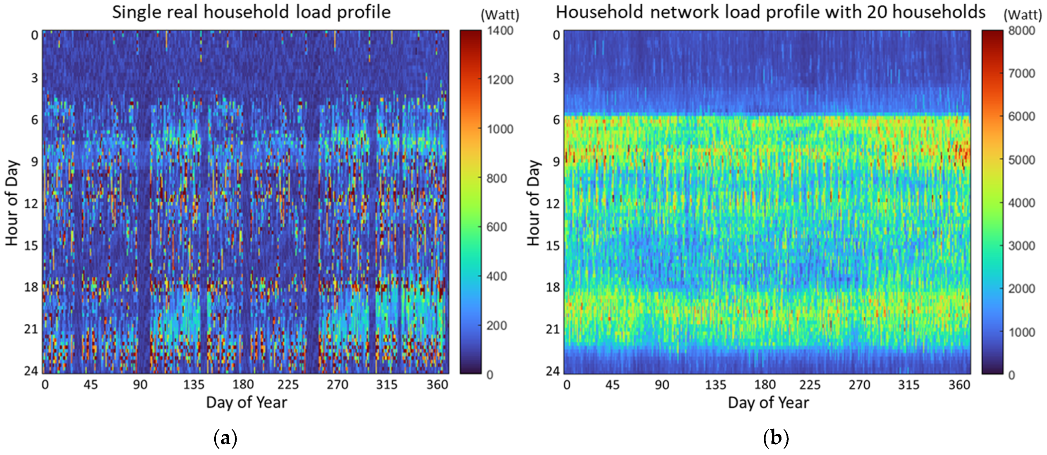
The load profile describing the load characteristics of the urban quarter solution is shown in Figure 3b. As seen in this figure, the load profile for the quarter solution, which included 20 households, was more consistent or even balanced in comparison with the load profile of a single household. This resulted in the necessity of a smaller dimensioning of the components, rather than building an energy system for every household on its own.

The aim of the urban quarter solution was to ensure a considerable degree of self-sufficiency in the households. For the PV system layout, it was assumed that all households in the district had the same PV system that faced south and was installed with an elevation angle of 45°; thus, the PV systems were installed under the same conditions and installation regulations as those of the individual households.

In order to make the urban quarter solution comparable with the private household solution, standardization was performed. The basic conditions were defined as each household having an energy demand for household electricity of 2500 kWh, a heat demand of 4000 kWh, and a hot water demand of 1000 kWh. The quarter solution had 20 times the energy demand. Thus, the urban quarter solution differed from the private household solution only in that there was a different energy distribution with more uniform energy consumption. For the load profiles of the private households, synthetically generated load profiles were used, which were created by using the LPG. The different load profiles represented different energy use behaviors of different household constellations. The key criteria were the numbers and types (children or adults) of people living in the household and their attendance behavior, which depended on their employment status. A total of 10 different household types were used, duplicated, and then offset by one week to achieve 20 different households.

In order to perform a comparison between the quarter solution and the household solution, the determined annual simulation results of the key parameters (grid feed-in, grid purchase, H2 utilization, energy towards the ELY, etc.) of the 20 private households were summed up and then compared with the annual values of the simulation results of the quarter solution. The simulation results are shown in

Table 4. Results of the parameter study for the urban quarter solution.

	Sum of All Individual Household Solutions	Urban Quarter Solution with One ELY	Urban Quarter Solution with Two ELYs
Overall energy demand (in kWh)	99,180	98,125	97,964
Electrical energy production by FC (in kWh)	28,760	27,457	27,347
Energy towards ELY (in kWh)	76,309	75,875	77,533
Grid feed-in (in kWh)	7294	7380	5735
Grid purchase (in kWh)	1055.09	58.98	59.64
Required ${\mathrm{H}}_2$ (in kg)	1559.70	1458.6	1450.9
Produced ${\mathrm{H}}_2$ (in kg)	1676.3	1671.7	1650.10
ELY—Operation hours during one year	1536.9	1559.7	1909.20|715.57
ELY—Overall years until EOL	15.28	15.41	11.74|32.89
ELY—Overall operation hours until EOL	23,481	24,042	22,416|23,535
FC—Operation hours in one year	2711	2645	2664
FC—Overall years until EOL	16.00	15.98	16.01
FC—Overall operation hours until EOL	43,393	42,267	42,653
LIB—Overall full cycles in one year	104.82	96.09	96.17
LIB—Overall years until EOL	9.18	9.34	9.35

.

The simulation calculated an ${\mathrm{H}}_2$ production quantity of 1671.71 kg for the quarter solution and, thus, an almost identical production quantity to that of the household solution. The ELY’s voltage efficiency was nearly the same in both cases. However, typically, a larger ELY system such as that in the quarter solution can also be expected to have a higher voltage efficiency (efficiency of the ELY stack). After modeling an ELY with an average efficiency of 75%, as opposed to the average efficiency of 70.14% for the household system, there was a 5.5% increase in the adjusted ${\mathrm{H}}_2$ production from 1676.3 kg to 1768.6 kg. In this context, the adjusted ${\mathrm{H}}_2$ production quantity is used not only because the production quantity is increased by the factor of the increase in efficiency, but also because there is increased energy consumption by the compressor, which, in turn, results in a lower energy available for the ELY. This lowers the ${\mathrm{H}}_2$ production quantity of the ELY. Neglecting economies of scale, there was, consequently, no apparent difference in the ${\mathrm{H}}_2$ production quantity between the quarter and household solutions.

The situation was different, however, for the ${\mathrm{H}}_2$ demand for the FC. The FC was modeled here under a constant power and efficiency behavior for the quarter and household solutions. Overall, the ${\mathrm{H}}_2$ demand for the quarter solution was 6.5% lower.

Next, the results of the simulation with two smaller ELYs instead of a large one are presented. It turned out that the first smaller ELY, which was in operation often, had a lower average efficiency compared to that of the large ELY. This was mainly due to the higher degree of utilization. The second ELY was turned on as soon as the first ELY reached the nominal power, which was already an adjustment because the utilization up to the maximum power in the simulation led to an intense decrease in the lifetime. As expected, the feed-in to the power grid was lower when two ELYs were used instead of one large ELY; though it was 22.3% lower, the proportion was less significant than expected. Overall, the amount of ${\mathrm{H}}_2$ produced even decreased by 1.3% from 1676.27 kg to 1650.07 kg when compared with that when using a single ELY. The use of two ELYs, in which the first ELY experienced a higher degree of utilization, was accompanied by a lower efficiency, resulting in this slight decrease in ${\mathrm{H}}_2$ production.

The most important comparative parameter was the lifetime of the ELYs. When using two ELYs, the first ELY had an expected lifetime of 11.74 years, while the second ELY had a theoretical lifetime of 32.89 years, neglecting standstill aging and calendar aging. The second ELY was in operation for only 715.57 h with an average current density of 1.46 A/cm². In contrast, the first ELY was in operation for 1909.15 h, with 612.95 h having an average current density of 1.69 A/cm². In contrast, the lifetime of the 100 kW ELY was 15.89 years. In summary, there were no significant positive effects when using two smaller ELYs instead of one large ELY. It was the lower expected lifetime of the first small ELY that called the benefit into question, although something can probably be gained here with a more sophisticated control system in which the two ELYs are operated in a more balanced manner with lower current densities.

3.5. Results of the Parameter Study of Weather Variations

In another study, the influence of weather data was investigated. For this purpose, weather data from four different years were used. In addition to the weather data (temperature, wind speed, and irradiation), a different heat demand profile was also taken into account in each case, as this is directly related to the temperature curve. The location (Würzburg, Germany) and the level of energy demand (household electricity and heat demand) remained identical. The years 2014 to 2017 were investigated. The energy requirements correspond to those of the standard household, as described in Section 3.

Figure 11 shows the hydrogen demands (a) and hydrogen productions (b) of the four simulations by month. According to this figure, production and demand varied slightly by month. The overall yearly hydrogen demand was lowest in 2014 with 67.93 kg and highest in 2016 with 79.87 kg (a difference of 17.6%). Hydrogen production, on the other hand, varied by only 7.6%: 78.52 kg in 2014 and 84.52 kg in 2015. The solar irradiance for the respective years, on the other hand, diverged only marginally, but showed differences when considered on a month-by-month basis (see Figure 11c).

Figure 12 shows the monthly hydrogen demand (a) and hydrogen production (b) as a function of the monthly solar irradiance. With a coefficient of determination of 0.9219 for (a) and 0.9539 for (b), the curves show a very good approximation to the measurement points. The deviations between the course of the curves and the measuring points are mainly due to variations in the energy demand of the corresponding months, but also the temporal availability of energy production in relation to the energy demand plays a role. The solar irradiance corresponds to the irradiance actually received by the PV system surface when the module is tilted by 45°. The values to be read can thus be applied to any surface, provided that the actual expected monthly solar irradiation on the surface is known. From a solar irradiation of about 143 kWh/m² per month, hardly any hydrogen demand can be expected, while below 25 kWh/m² per month, hardly any hydrogen production takes place. The curve of the hydrogen demand depends on the energy demand, whereas mainly the heat demand plays a role. The size and power of the PV system play a major role in hydrogen production. In this example, 26 modules with 310 W_p each were used with a conversion efficiency of 18.6% under STC and a southern orientation with an angle of inclination of 45°.

3.6. Results of the Parameter Study for Variations in Heat Demand

For this parameter study, a standard real measured domestic electricity load profile was considered. The focus of this parameter study was on variations in the heating demand; only the space heating demand was varied, and the water heating demand was not. The water heating demand was assumed to be constant at 1000 kWh per year, while the space heating demand was increased in 4000 kWh increments from 4000 kWh to 20,000 kWh. As a result, the entire system layout had to be redesigned as the heat demand increased. The increase in heat demand led to a shift in energy demand towards the winter, which resulted in an increase in the energy to be provided via the ${\mathrm{H}}_2$ chain.

The results of this parameter study are shown in

Table 5. Results of the parameter study of variations in heat demand.

	Gross Heat Demand in kWh
	4000	8000	12,000	16,000	20,000
Electrolyser nominal power	3.6 kW	5 kW	7 kW	9 kW	10 kW
Fuel cell nominal power	700 W	1200 W	2000 W	3000 W	3500 W
PV system size (orientation towards South; ${\gamma }_E=45°$)	24 modules	34 modules	44 modules	54 modules	64 modules
LIB capacity	20 kWh	20 kWh	25 kWh	30 kWh	35 kWh
Overall PV energy generation (in kWh)	8508.64	12,053.90	16,308.22	19,144.43	22,689.70
Overall energy demand (in kWh)	4754.45	6394.07	8115.28	9909.51	11,547.24
Electrical energy demand for space heating with a heat pump (in kWh)	1416.72	2948.96	4503.25	6052.58	7588.37
Electrical energy generation by the fuel cell (in kWh)	1377.54	2213.04	3007.20	3952.05	4743.45
Heat demand savings by fuel cell waste heat (in kWh)	707.74	1141.32	1522.53	1923.19	2348.76
Required ${\mathrm{H}}_2$ (in kg)	74.67	117.53	157.78	203.56	245.52
Produced ${\mathrm{H}}_2$ (in kg)	78.37	118.60	159.62	207.14	242.06
Net hydrogen utilization (in kg) (a positive value indicates ${\mathrm{H}}_2$ deficit)	−3.71	−1.07	−1.83	−3.58	3.46
Share of direct PV use	38.73%	35.74%	33.73%	32.21%	31.55%
Share of direct FC use	19.96%	27.27%	30.36%	33.09%	33.83%
Share of battery storage use (charged by PV energy)	32.39%	29.95%	29.58%	28.28%	27.77%
Share of battery storage use (charged by FC energy)	8.13%	6.63%	6.04%	6.13%	6.54%

. The heat demand was mainly covered by a heat pump, in addition to a small part that was covered by the FC via waste heat recovery, resulting in a reduction in the absolute electrical energy demand. The usable waste heat fraction increased quite proportionally with increasing heat demand and the increase in the FC nominal power.

However, as the heat demand increased, the fraction of energy directly supplied by the PV system decreased from 38.73% to 31.55%. In turn, the percentage that was directly covered by the FC significantly increased from 19.96% to 33.83%. This was due to the fact that with an increasing proportion of heat demand in the total energy demand, a stabilization of the load to be covered occurred, which could then be directly covered to a higher extent at a constant FC output.

Overall, the hydrogen demand significantly increased, but it did so linearly with the increase in the heat demand from 74.67 kg to 245.52 kg. The coefficient of determination here was 0.9997. The following formula for the hydrogen demand $m_{H_2}$ was obtained as a function of the heat demand:

$$f\left(x\right)=0.0107x+31.5$$

The hydrogen demand was divided by month for the different heat demands, as shown in Figure 13.

Following to principle of Figure 12, Figure 14 shows the hydrogen demand and production curves under different heat demands and PV system designs, respectively. For the hydrogen demand (a), there is a largely uniform upward shift in the curve as the heat demand increases, while the hydrogen production curve (b) shifts largely uniformly as the PV system size increases. The amount of PV modules was selected according to the minimum required for self-sufficiency. If fewer PV modules were used, this resulted in a larger increase in the hydrogen demand at a low solar irradiance, as well as a less steep increase in hydrogen production.

If both space heating and water heating requirements were neglected, the linear relationship between the hydrogen demand and household electricity shown in Figure 15 was determined. The measurement points were made by further simulations with a gradual increase in the household electricity, choosing the lowest possible design that ensured self-sufficiency. The data were simulated using the input data for 2015 for the location of Würzburg (Germany).

4. Discussion

This section discusses the findings described in Section 3 regarding the optimal system design and the influences of various load characteristics, system scaling, and heat demand variations. In Section 3.2, it was shown that complete self-sufficiency of the power system was only achieved if the FC was designed according to the 99.8th percentile of the load distribution. In contrast, however, a self-sufficiency of 99.44% was achieved with the design according to the 50th percentile, when used with an appropriate short-term storage unit. This suggests that the larger FC should be dispensed with and that appropriate energy management system measures should be taken in the event of a short-term energy deficit, e.g., by operating the FC above the rated power for a short time, by load balancing, or by shifting the load.

The ELY should also be adapted to the application at hand, the intended installation site, the size of the PV system, and the expected load, especially during the summer months. It was shown that if the design is inadequate—either too large or too small—the production costs per kg of ${\mathrm{H}}_2$ can quickly increase. In addition, if the layout is too large, the degree of self-sufficiency of the energy system also decreases again, since a larger layout is also accompanied by an increase in the minimum power, which can affect the ${\mathrm{H}}_2$ production. If the layout is too small, the same effect occurs, but here, the ${\mathrm{H}}_2$ production is limited by the maximum power. In the case of the ELY in particular, further investigations are advisable, especially with regard to optimized power control, which is possibly also in combination with intermediate battery storage. In particular, with the combination of a lifetime and economic analysis, more meaningful statements can be achieved.

Particularly when using a small LIB, it was shown that the load characteristics had a significant influence on the ${\mathrm{H}}_2$ demand and production, as well as on the utilization shares of the forms of energy storage. In contrast, with an increase in the LIB storage capacity, the difference in ${\mathrm{H}}_2$ demand and production significantly decreased. This showed that with the adjustment of the LIB storage capacity, increased unification of the system design becomes possible despite the different load characteristics. The results from Section 3.3 also show the advantages of hybrid energy storage consisting of short-term storage and long-term storage with regard to the required ${\mathrm{H}}_2$ storage demand. With all else being equal, the ${\mathrm{H}}_2$ demand significantly decreased by an average of 19.8% when the LIB storage capacity was increased from 6 kWh to 10 kWh. This also increased the predicted FC lifetime by an average of 80%.

The investigation of the quarter solution with a comparison of the use of two small ELYs instead of one large ELY did not reveal any significant positive effects, but rather revealed negative effects related to the overall stack lifetimes. It was found that a significant increase in lifetime could be achieved by utilizing the first ELY not at its maximum power, but only at its rated power. Having an appropriate load control was also advantageous here. With the energy demand of the household network being otherwise assumed to be the same, compared with the sum of all separate households, a higher energy coverage reliability was shown due to the more evenly distributed load curve. The ${\mathrm{H}}_2$ demand also somewhat decreased. Otherwise, the advantageousness of the quarter solution could only be supported by economies of scale, e.g., in the system efficiencies.

The inclusion of the heat demand significantly increased the hydrogen demand, even for small heat demands. Even at an increase of about 2000 kWh of electric energy demand for the heat pumps, the hydrogen demand was more than double of that when meeting only the domestic electricity demand. For every increase of 1000 kWh of electrical energy demand for space heating, the hydrogen demand increased by approximately 28 kg for the designated location.

5. Conclusions

When designing the ELY and the FC, their lifetime should always be taken into account. An economic analysis showed considerable differences when the lifetime of the components related to sizing and the system layout is considered. At an average utilization of about 50% during operation, the specific costs per kilogram of hydrogen produced were the lowest in the application case considered here. In this case, no power control was used, but the ELY was started at the moment when an energy surplus was available, and the minimum power of the ELY was exceeded. Consequently, even with an average utilization of about 50%, high power records of the ELY could occur. In this context, a further increase in lifetime is achievable by means of power control, which supplies the ELY more evenly.

The storage capacity increase in the LIB does not allow an unlimited reduction in the hydrogen demand. A previous paper [3] has already showed that in a design to cover 4000 kWh in heat demand, an increase in the LIB capacity from 20 kWh to 40 kWh no longer had a large effect (a reduction from 77.64 kg to 69.72 kg in hydrogen demand). In contrast, with an LIB capacity of 5 kWh, a much higher hydrogen demand of 105.07 kg occurred.

An FC designed according to the 50th percentile of the power distribution showed a very high degree of self-sufficiency of 99.44%. In contrast, complete self-sufficiency was only achieved with a design according to the 99.8th percentile. In particular, the combination with a sufficiently large LIB proved to be useful in order to save costs for the FC.

The hydrogen demand increased from 74.67 kg at 4000 kWh of annual heat demand to 245.52 kg at 20,000 kWh of heat demand when the heat demand was covered by a heat pump and waste heat. Hereby the percentage that was directly covered by the FC significantly increased from 19.96% to 33.83%. Neglecting the heat demand, the hydrogen demand to cover the household electricity consumption of 2500 kWh annually was about 31.5 kg. However, this value strongly depends on the capacity of the short-term LIB storage, as shown in the study of different load characteristics. If the LIB capacity chosen is too small, the hydrogen demand varies significantly depending on the load characteristics: for an LIB capacity of 6 kWh (65% usable), it varied between 46.01 and 37.67 kg. With an LIB capacity of 10 kWh (65% usable), it varied only between 34.06 and 31.99 kg and thus showed a high consistency despite different load characteristics. A second effect became apparent: with the increase in the LIB storage capacity, the hydrogen demand dropped considerably, by an average of 19.8%.

Depending on the year under consideration, differences in the hydrogen demand and hydrogen production became apparent. In the four years considered, 2014 to 2017, the hydrogen demand diverged by 17.6%, while hydrogen production diverged by only 7.6%. Accordingly, a safety margin should always be estimated when designing the system, especially the hydrogen storage system, the PV system, and the ELY, if full self-sufficiency is the goal. A high correlation between the solar irradiance and hydrogen demand with respect to hydrogen production was found, as shown in Figure 12 and Figure 14. The solar irradiance in relation to the hydrogen demand showed a relationship similar to an exponential function with a negative exponent with a coefficient of determination of 0.9219. The solar irradiance in relation to hydrogen production showed a correlation approximating a power function with a coefficient of determination of 0.954.

These results provide insight that a targeted layout tailored to an application is important and can be simulated very realistically with the developed model. In addition to the dimensioning of the components, the load characteristics and the load distribution over a year (expressed by heat demand variations) play a decisive role and should, therefore, be considered. Our results confirmed that the lifetime of the components depends significantly on their layout and the energy management system. In the context of further investigations, it is necessary to integrate an economic efficiency analysis as a further evaluation criterion and, thus, to make different system designs comparable in terms of costs. Further studies with a larger simulation scope and a different focus for our investigation are also planned.