Drone Polariscopy—Towards Remote Sensing Applications ^†

Abstract

Remote sensing is critical for a wide range of applications, including ocean and wave monitoring, planetary exploration, agriculture, and astronomy. We demonstrate a polariscopy concept that is able to determine orientation of patterns below the optical resolution limit of a system. This technique relies on measuring at least four different polarisation angles and calculating the orientation from this set of intensity information. It was initially demonstrated on the Infrared Microspectroscopy Beamline at the Australian Synchrotron using IR light in transmission. Using a monochrome polarising camera mounted onto a drone as a remote sensing platform analogue, orientation information was extracted from 3D-printed targets in reflection. The images were taken at an altitude where conventional imaging could not resolve the test patterns. The system had a 3.33 mm ground resolution. Patterns consisting of 0.5 mm lines spaced 0.5 mm apart were detected using the method, demonstrating the capability of detecting features over six times smaller than the resolution limit. In the interest of moving towards high-speed data acquisition and processing, two methods for processing the image are compared—an analytical and a curve fitting method.

1. Introduction

The ability to detect periodic features below the resolution limit of a system is valuable to all forms of imaging. This is especially important in areas such as remote sensing, where the cost of launching a satellite is dependent on its mass. Polarisation information adds an additional dimension to image data and has shown value in machine vision, where it is utilised for analysis of reflections [1]. In remote sensing, the orientation detection of waves is studied using synthetic aperture radar (SAR). The polarisation orientation has been used on an existing resolved image [2,3]. These satellites need large, heavy antennas to achieve their resolutions. However, in such a contexts, polarisation has not been used for diffraction-limited imaging of anisotropy. A method using Fourier transform infrared spectroscopy was developed and transferred to the Infrared Microspectroscopy Beamline at the Australian Synchrotron, which demonstrated anisotropy recognition and mapping below the spatial resolution limit for the first time [4,5]. The method described—the 4-pol method—involves measuring the sample at four polarisation angles (0${}^{\circ }$, 45${}^{\circ }$, 90${}^{\circ }$, and 135${}^{\circ }$ ($-{45}^{\circ }$)). In addition to molecular anisotropy, the orientation of a circular grating with a 200 nm pitch and 100 nm line width was detectable with a system resolution of 5 $\mathsf{\mu }$m, a 25 × difference [6]. To demonstrate the ability of the 4-pol method to move beyond the IR wavelengths and microscopy scale, a 4-pol visible light camera was used to show orientation detection in the visible wavelength range [7]. In this preliminary study, we extended the method even further and mounted the camera on a drone, which functioned as a remote sensing platform analogue and operated in reflection mode.

2. Materials and Methods

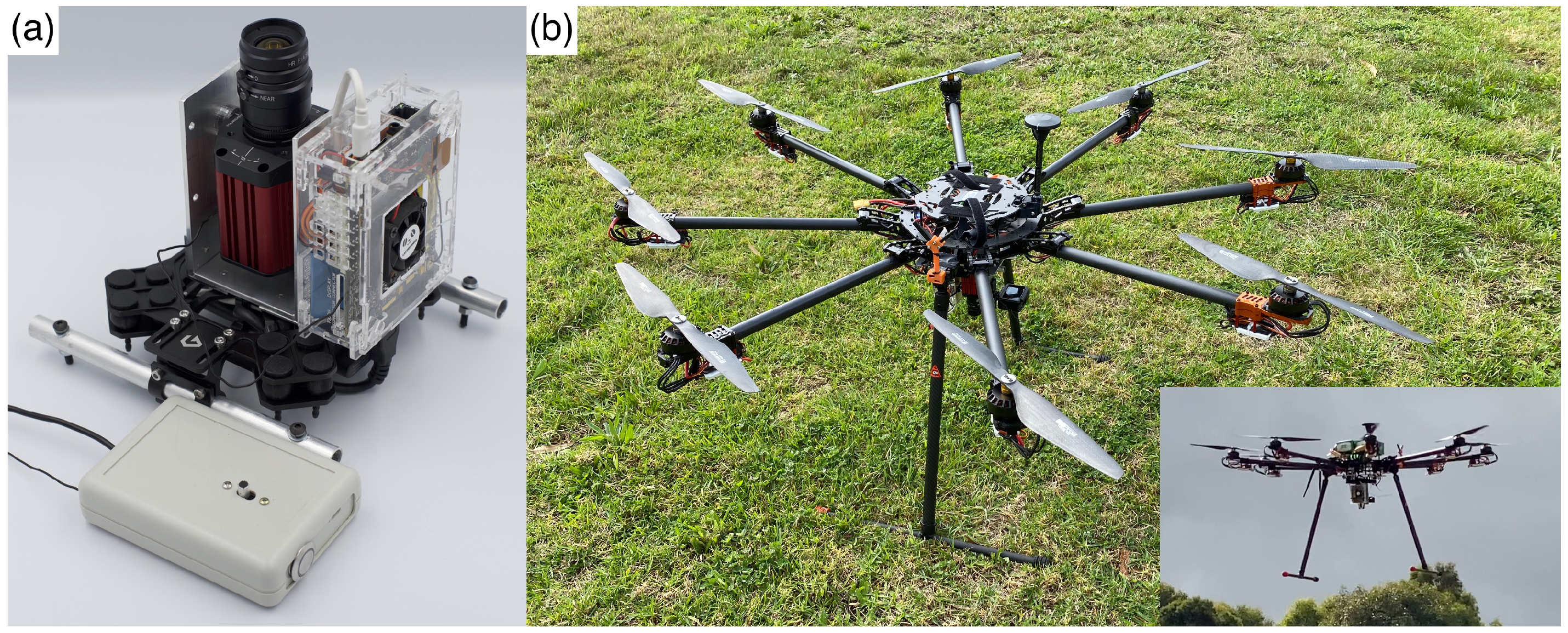
2.1. Drone Flight with Polarisation Camera

The CS505MUP monochrome polarisation camera (Thorlabs Inc.) has a 2448 × 2048 pixel sensor with micro-polarisers directly over each 3.5 $\mathsf{\mu }$m pixel. Each 2 × 2 group of pixels provides 0${}^{\circ }$, 45${}^{\circ }$, 90${}^{\circ }$, and 135${}^{\circ }$ intensity information for a total of 1224 × 1024 for each polarisation angle. A Navitar MVL8M23 f/1.4, 8 mm lens was attached to the camera, which was then mounted on a custom mounting rig which provided vibration damping, a battery, a LattePanda computer with a receiver, and a GoPro video camera (Figure 1a). This rig was then bolted under a Kraken 130V2 octocopter drone platform (Figure 1b). After takeoff, the acquisition was remotely triggered to conserve power and storage space. To account for different lighting conditions, the camera was programmed to record a bursts of 10 images at varying exposure times, every 30 s. The drone was flown up in steps of 20 m and hovered for 1 min to ensure a full set of images were acquired at each altitude. 3D-printed targets (Figure 2) consisting of 0.5 mm lines with a 1 mm pitch (one circular with an Archimedean spiral and one rectangular with different orientations in each quadrant) were set up on the ground as points of known orientation. The diameter of the circle was 20 cm and the dimensions of the rectangle were 24 × 20 cm.

2.2. Data Processing

The data were subsequently converted to intensity and orientation information using two methods—analytical and curve fitting [4,8]. For the analytical solution, the intensity is given by

$$I=\frac{I_{0^{\circ }}+I_{{45}^{\circ }}+I_{{90}^{\circ }}+I_{{135}^{\circ }}}{2},$$

(1)

where I is the image intensity and $I_{{\theta }^{\circ }}$ is the intensity at a specific polarisation angle. The orientation (azimuth) is given by

$$\psi =\frac{1}{2}\arctan 2\left(\frac{I_{{45}^{\circ }}-I_{{135}^{\circ }}}{I_{0^{\circ }}-I_{{90}^{\circ }}}\right),$$

(2)

where arctan2 is the four-quadrant inverse tangent. The equation used for fitting was

$$I\left(\theta \right)=Acos(2\theta -2\psi )+c,$$

(3)

where $I\left(\theta \right)$ is the intensity at a specific polariser angle, A is a factor proportional to the degree of polarisation, $\theta$ is the polariser angle, $\psi$ is the azimuth, and c is a factor proportional to I. The bounds of the fit were $0<A<5$, $-\frac{\pi }{2}<\psi <\frac{\pi }{2}$, and $-5<c<5$. The initial guesses were $A=1$, $\psi =0$, and $c=1$. In all cases, these were the values used for all pixels.

3. Results and Discussion

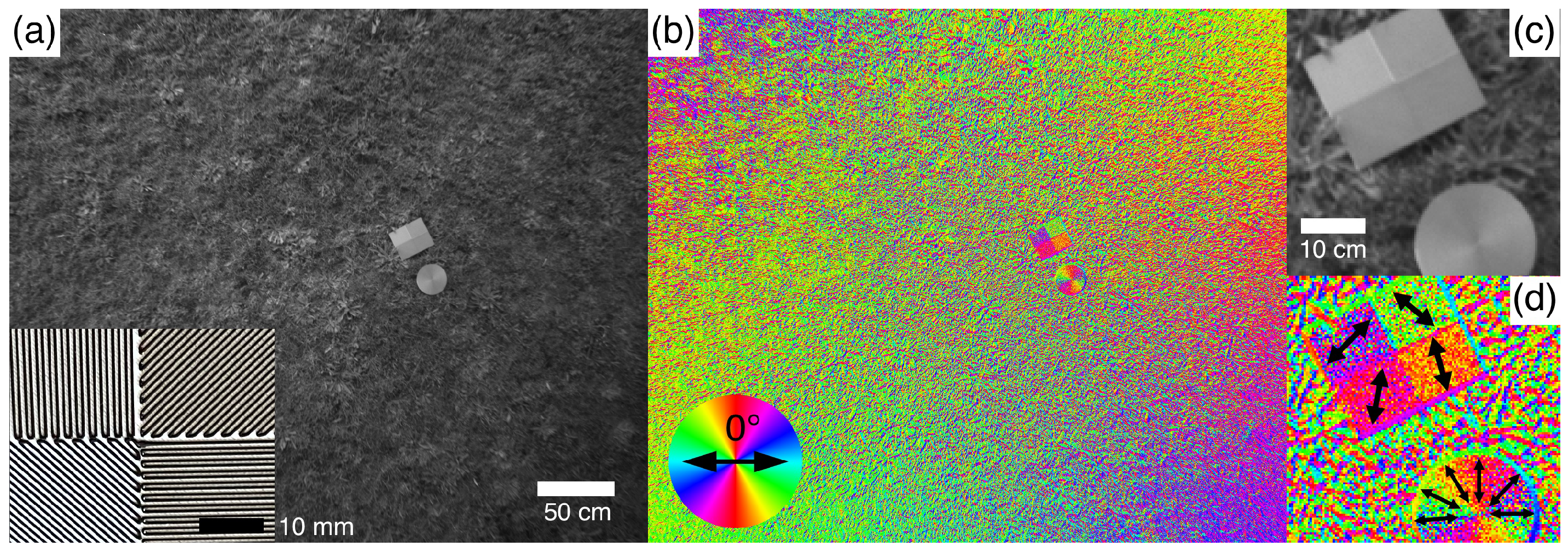
3.1. Orientation Determination

Figure 2a shows an intensity image, calculated with Equation (1), at an altitude of approximately 4 m, and the inset shows a photo of 3D-printed lines on the rectangular target. This height is equivalent to 3 pixels/cm in the image or 6 pixels/cm over the full sensor (calculated using the 20 cm diameter circle as a reference). The highest theoretical resolution of a sensor is when two points are imaged onto separate neighbouring pixels. Naively for the above sensor with a pixel size of 3.5 $\mathsf{\mu }$m, the sensor resolution $R_{\mathrm{sensor}}$ can be considered 3.5 $\mathsf{\mu }$m, although physical limitations preclude this. The polarisation image (equivalent pixel size of 6.9 $\mathsf{\mu }$m) has half the resolution of the full sensor. The magnification factor

$$m=\frac{\mathrm{Sensor}\mathrm{width}}{\mathrm{Image}\mathrm{width}}$$

between the object space and sensor can be used to calculate the maximum object resolution $R_{\mathrm{object}}$. For the image in Figure 2a,

$$m=\frac{8.445\mathrm{mm}}{4080\mathrm{mm}}=0.00207.$$

Hence,

$$R_{\mathrm{object}}=\frac{3.45\mathsf{\mu }\mathrm{m}}{0.00207}=1.67\mathrm{mm}$$

for the full sensor and 3.33 mm for the polarisation intensity image.

Since the spaces between the lines were 0.5 mm, the lines could not be resolved in the image. Applying Equation (2) resulted in Figure 2b, which shows colours representing the azimuth angle with 0${}^{\circ }$ defined as shown in the bottom left. It is evident that each quadrant of the rectangular target shows a different orientation, and the circular target shows radial changes. Figure 2c,d shows enlarged versions of the region of interest. Arrows in Figure 2d show approximate azimuth orientation. The azimuth is orthogonal to the orientation of the printed lines for both rectangular and circular targets. This is in contrast to transmission mode, where the calculated azimuth is parallel to the alignment [6]. However, the fact that the azimuth is consistent still indicates that the 4-pol method detects orientation that cannot be resolved by the optics in reflection. This system, with a theoretical 3.33 mm resolution, was able to determine the orientation of 0.5 mm lines spaced 0.5 mm apart, demonstrating detection of patterns over six times smaller than the resolution limit. It also shows that it works in cases where either the detected features are much smaller or much larger than the wavelength of the probing light. The difference in azimuth alignment might have been due to the illumination from the sky, since polarisation varies with angle from the sun [9].

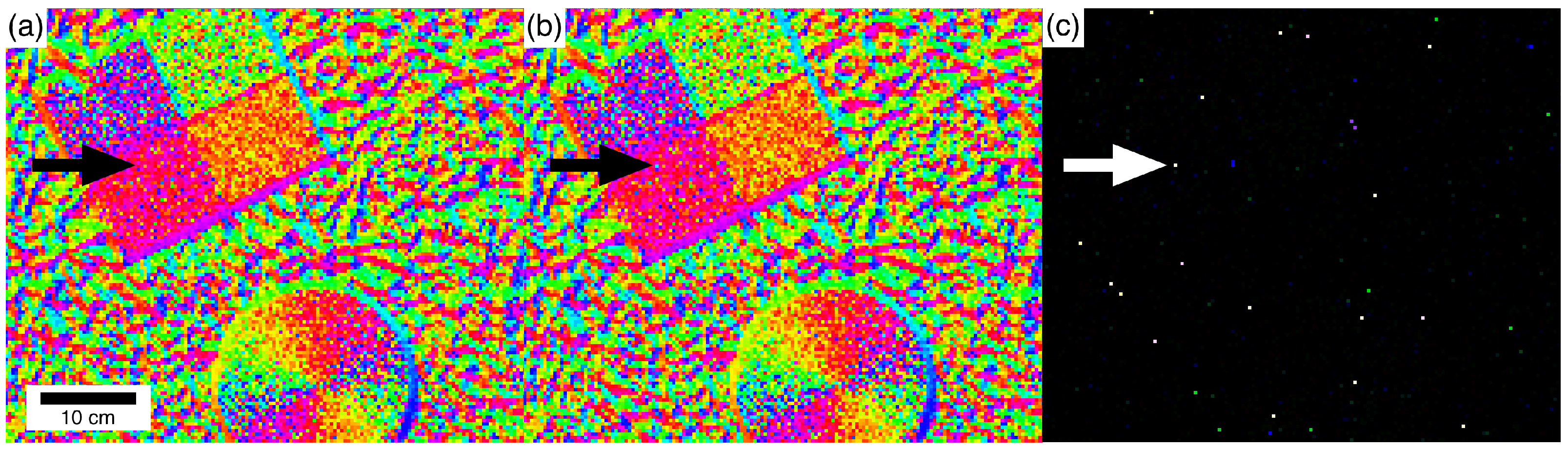
3.2. Data Processing Method

There are cases wherein there is a low signal-to-noise ratio, the angle of a polariser cannot be set precisely, or the polarisation combinations are not 45${}^{\circ }$ apart. The analytical method cannot accommodate these, and so curve fitting can be used to determine the azimuth and intensity. This comes at a time cost, however. While Equations (1) and (2) can be vectorised so the calculation can be performed on an entire image at once, curve fitting needs to be done for each pixel. As a single-thread process, the analytical method takes <1 s to process 1 frame. The same frame using curve fitting takes over 3 h.

While the fitting method is slow, it ultimately returns the very similar results to the analytical method, when the bounds are set correctly. Figure 3a shows an enlarged cropped section from Figure 2b, and Figure 3b shows the same area but calculated by fitting each pixel. At a glance, they are indistinguishable; however, Figure 3c shows that there are several pixels which are different. These differences are not very significant, as the number of pixels that do not agree are few. The time disparity demonstrates that the fitting method should only be used when a great number of polarisation measurements are needed—when the signal-to-noise ratio is low.

4. Conclusions

The 4-pol method was successfully transferred from the Infrared Microspectroscopy Beamline to a drone platform. It was shown that orientation could be determined even when the aligned features (0.5 mm lines 0.5 mm apart) could not be spatially resolved (3.33 mm resolution). This demonstrated that patterns over six times smaller than the system’s resolution limit could be extracted from the image. The calculated azimuth was orthogonal to the alignment direction, and the reason for this requires further study. This is a stepping stone towards satellite-based remote sensing using the same technique, and opens up possibilities for ocean monitoring, planetary observation, and astronomy, where orientation information is important.

References

1. Atkinson, G.A.; Ernst, J.D. High-sensitivity analysis of polarization by surface reflection. Mach. Vis. Appl. 2018, 29, 1171–1189. [Google Scholar] [CrossRef] [Green Version]
2. Schuler, D.L.; Lee, J.S.; Kasilingam, D.; Pottier, E. Measurement of ocean surface slopes and wave spectra using polarimetric SAR image data. Remote. Sens. Environ. 2004, 91, 198–211. [Google Scholar] [CrossRef]
3. Viana, R.D.; Lorenzzetti, J.A.; Carvalho, J.T.; Nunziata, F. Estimating energy dissipation rate from breaking waves using polarimetric SAR images. Sensors 2020, 20, 6540. [Google Scholar] [CrossRef] [PubMed]
4. Hikima, Y.; Morikawa, J.; Hashimoto, T. FT-IR Image Processing Algorithms for In-Plane Orientation Function and Azimuth Angle of Uniaxially Drawn Polyethylene Composite Film. Macromolecules 2011, 44, 3950–3957. [Google Scholar] [CrossRef]
5. Ryu, M.; Balčytis, A.; Wang, X.; Vongsvivut, J.; Hikima, Y.; Li, J.; Tobin, M.J.; Juodkazis, S.; Morikawa, J. Orientational Mapping Augmented Sub-Wavelength Hyper-Spectral Imaging of Silk. Sci. Rep. 2017, 7, 1–10. [Google Scholar] [CrossRef] [PubMed] [Green Version]
6. Honda, R.; Ryu, M.; Moritake, M.; Balčytis, A.; Mizeikis, V.; Vongsvivut, J.; Tobin, M.J.; Appadoo, D.; Li, J.L.; Ng, S.H.; et al. Infrared Polariscopy Imaging of Linear Polymeric Patterns with a Focal Plane Array. Nanomaterials 2019, 9, 732. [Google Scholar] [CrossRef] [PubMed] [Green Version]
7. Ng, S.H.; Anand, V.; Duffy, A.; Babanin, A.; Ryu, M.; Morikawa, J.; Juodkazis, S. Remote-sensing concept using polariscopy for orientation determination below the spatial resolution limit. In Photonic Instrumentation Engineering VIII; Soskind, Y., Busse, L.E., Eds.; SPIE: Bellingham, WA, USA, 2021; Volume 1169306, p. 4. [Google Scholar] [CrossRef]
8. Ryu, M.; Nishijima, Y.; Morimoto, S.; To, N.; Hashizume, T.; Matsubara, R.; Kubono, A.; Hu, J.; Ng, S.H.; Juodkazis, S.; et al. Hyperspectral Molecular Orientation Mapping in Metamaterials. Appl. Sci. 2021, 11, 1544. [Google Scholar] [CrossRef]
9. Coulson, K.L. Polarization and Intensity of Light in the Atmosphere; A. Deepak: Hampton, VA, USA, 1988. [Google Scholar]
Figure 1. (a) Photograph of the polarisation camera in its mounting rig along with a remote control. (b) Preflight photo of the octocopter with camera module attached underneath. Inset shows the drone and camera just after takeoff.
Engproc 11 00046 g001
Figure 2. (a) Intensity image of 3D-printed targets on a grass field at an altitude of ∼4 m. Inset shows a photo of the centre of the rectangular target showing the orientation in each quadrant. (b) Corresponding azimuth map with the colours indicating azimuth angle. (c) Enlarged intensity image of the targets. (d) Enlarged azimuth image of the targets with black arrows indicating approximate calculated azimuth orientation.
Engproc 11 00046 g002
Figure 3. (a) Azimuth image calculated using Equation (2). (b) Azimuth image calculated by fitting Equation (3). (c) Images (a,b) overlaid with the difference image blend mode showing pixels that are different in colour and pixels which are the same as black. Arrows are eye guides to one pixel which is different.
Engproc 11 00046 g003
Publisher’s Note: MDPI stays neutral with regard to jurisdictional claims in published maps and institutional affiliations.