Comparing New Wireless Sensor Network Protocols through Simulation and Data Analysis ^†

Abstract

The resource-constrained nature of wireless sensor networks (WSNs) creates a number of difficulties in their operation and design that lower their performance. However, distinct applications with unique constraints in their nature make it more difficult for such resource-constrained networks to meet application objectives. These issues can be observed at various WSN layers, from the physical layer up to the application layer. Routing protocols are primarily focused on WSN functioning at the routing layer. These obstacles make routing protocols perform worse, which lowers the performance of WSNs as a whole. This study’s objective is to pinpoint WSN performance issues and examine how they affect routing protocol performance. To this end, a detailed literature review was conducted to determine the problems influencing the performance of the routing protocols. Then, an actual investigation was carried out by simulating various routing protocols, taking into consideration these issues, in order to validate the impact of the discovered challenges from the literature. The findings are shown. On the basis of the findings from the empirical study and the literature review, suggestions are offered for a better protocol choice in light of the application nature and the problems that need to be addressed.

1. Introduction

There are many benefits to wireless communication over traditional wired networks, including the ability to create compact, affordable, low-power, and multi-functional sensing devices. These tiny sensors are characterized as sensors because they are capable of sensing, computing, self-organization, and communication. A sensor is a small device that senses the ambient conditions in its environment, collects data, and processes it to provide useful information that may be used to identify occurrences in the surrounding area. Using mesh networking protocols, these sensors can be joined together to create a network that communicates wirelessly across radio frequency channels. Wireless sensor network (WSN) is the term used to describe the grouping of these homogeneous or heterogeneous sensor nodes [1]. Sensor nodes can be placed in large numbers in an area that has to be explored due to their low cost, small size, and ease of deployment [2]. Weirdly, unlike other networks that get weaker and perform worse as their size increases, WSNs get stronger and perform better as the number of nodes increase. Additionally, the number of nodes in a network can be increased without any complicated settings. As a result, it is claimed that connectivity employing mesh networking will use node-to-node hoping to occupy any available communication link in pursuit of the destination. Due to all these important benefits, WSNs have a wide range of applications, including real-time tracking, weather forecasting, health care applications, military operations, transportation, and security.

WSN is a network made up of hundreds or thousands of tiny sensor nodes that can sense, compute, and communicate with one another and the base station. The four components that make up a sensor node’s functional architecture are the sensor, CPU, radio, and power. Three of these four units are in charge of completing a task, while the power unit provides energy for the entire operation. The sensing unit’s job is to measure environmental variables like temperature, humidity, and pressure [3,4]. The processing unit’s main duty is to process data (signals), and the communication unit’s job is to transmit data from the sensor unit to the user via the base station (BS) [5]. These tiny sensor nodes are dispersed around the study area to gather environmental data, process it, and send it to the base station [6].

One can assume that WSNs operate similarly to conventional wired or wireless networks by looking at their application domain. But in practice, things are very different since conventional wired or wireless networks have sufficient resources, including boundless power, memory, fixed network topologies, adequate communication ranges, and computing capabilities [7,8]. On the other hand, WSNs are resource-constrained in terms of their ability to use energy, compute, and store data [9,10]. Unfortunately, we have the same expectations for the WSNs as we have for regular computer networks despite the limited resources available.

Because WSNs have limited resources, several difficulties in their design and operation affect how well they work. Communication management, unattended operations, network longevity, and fault tolerance rank highly among these difficulties [11]. Therefore, these problems are subject to research in order to enhance WSN performance. On the other hand, effective resource utilization can considerably improve WSN performance. By concentrating on the elements involved in WSN operations, resource consumption can be improved. The resources of WSNs are undoubtedly influenced by communication. Node-to-node, node-to-BS, and BS-to-node communication are all part of the WSN communication pattern. For this communication, the best route is used.

2. Research Methodology

This portion of the essay presents the methods we chose for this study. Additionally, the rationale for choosing certain approaches is explained, as Figure 1. For this research, a mixed-method approach was adopted. A mixed-method methodology is a research approach that incorporates both qualitative and quantitative approaches, according to [8].

3. Simulation and Empirical Study

3.1. Simulation and Simulation Model

The first step in the simulation process is the creation of a model that represents either a theoretical or an actual system. The second step involves running the model through its paces on a digital computer, and the third step involves evaluating the results of running the model through its paces. Learning through simulation is the same as learning by doing, which means that in order to comprehend or learn about any system, we must first create a model for it and then run it. To begin with, we need to be familiar with the concepts of systems and models in order to comprehend a simulation model. A system is an entity that exists and acts in time, and a model is the representation of that system. This streamlined illustration of systems was utilized for it allows for a better understanding. The process of developing a simulation is iterative, and the end result is appropriate information and comprehension. The simulation process can be broken down into three distinct subfields: model design, model execution, and model analysis [10]. These subfields are depicted in the figure below.

3.1.1. Simulation Tool (OPNET)

The Optimized Network Engineering Tool (OPNET version 14.5) modeler is a network simulator that offers solutions for managing networks and applications. Some of these solutions include network engineering, research and development, operation, planning, and performance management. It can represent communication devices, protocols, and technologies, and it can mimic the performance of these technologies in a dynamic virtual network environment. These are some of its uses. Academic research in the field of OPNET technology offers support for wireless protocols, Mobile Ad hoc network protocols, and core network technologies [12].

3.1.2. Network Entities and Functions

The wireless local area network (WLAN) is the network that was created specifically for this simulation. This network is comprised of fundamental network entities, such as sensor nodes (both fixed and mobile) and a base station. Objects pertaining to application configuration, profile configuration, and mobility configuration are added and configured in order to facilitate application configuration and mobility of the nodes, as Figure 2.

Nodes perform some sort of processing and then send the results either directly to the base station or to an intermediate node in a hierarchy. These nodes are referred to as submission nodes, and their number might vary based on the task that is intended for them.

4. Results and Analysis

The outcomes of our simulations are the topic of discussion and investigation in this paper. We have described our findings in light of the situations that we selected in two networks consisting of both stationary and mobile nodes. In a WSN, a data collection application is represented by a fixed node network, and an object-tracking application is depicted by mobility nodes. We have investigated two distinct possibilities with regard to both of these networks. Scalability was one of the features we included in the first scenario, whereas node failure was part of the second. The analysis of a fixed node network with scalability and subsequently with the existence of node failure was the first analysis we performed when we started talking about this topic. In addition to this, we analyzed the behavior of the protocols in each of these cases based on a set of performance measures. After that, we performed an analysis of mobile networks for the identical scenario, evaluating the protocols against the identically chosen metrics. We will draw a conclusion after conducting a comparison.

4.1. Fixed Nodes Scenarios with Network Size (Scalability) and Node Failure

We worked on two primary scenarios while using a network with fixed nodes. In the first scenario, we raised the number of fixed nodes in order to test how the protocols behaved as the size of the network changed. We achieved this by analyzing the WLAN metrics and the routing overhead. In the second scenario, we tested a small network consisting of 25 nodes and a large network consisting of 50 nodes for the same metrics while there was a random failure. Both of these hypothetical situations were devised with the intention of illustrating the data-gathering applications. As a result, all of the participating nodes in both sets of circumstances were judged to be fixed and submitting nodes, which meant that they communicated with the sink node at predetermined intervals. FTP was the application that was utilized for each and every scenario. The packet size that was utilized was 512 bytes, and the packet rate that was utilized was four packets per second, as

Table 1. Parameter vs. Value for 1st case.

Parameter	Value
Environment size	1000 × 1000 m
Number of nodes	25 and 50
Traffic type	Constant bit rate
Nodes type	Fixed
Packet rate	4 Packets/s
Packet size	512 byte
Number of Flows	25 and 50
Simulation time	3600 s
Number of submission hosts	25 and 50
Number of receivers	One

.

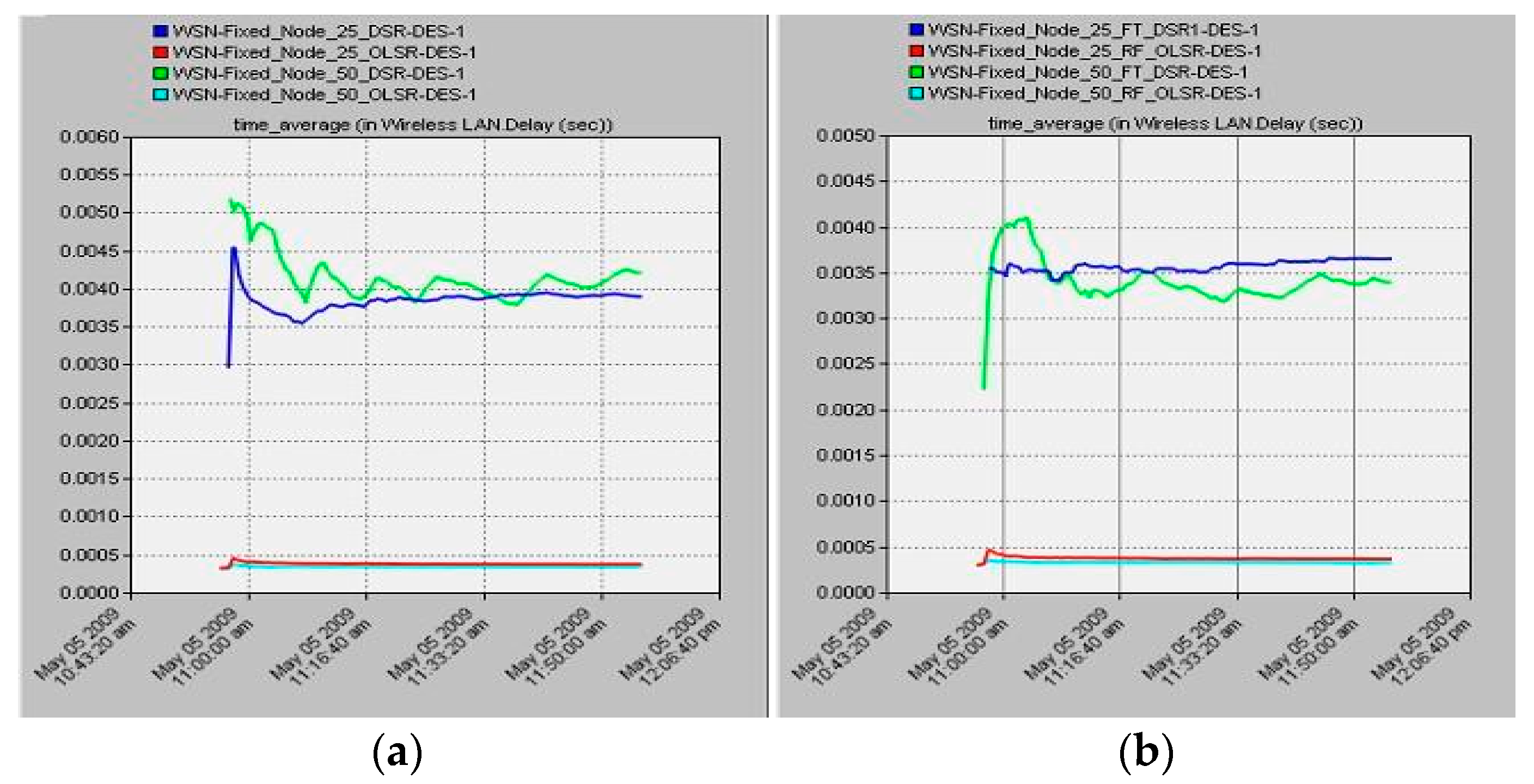
4.2. End-to-End Delay

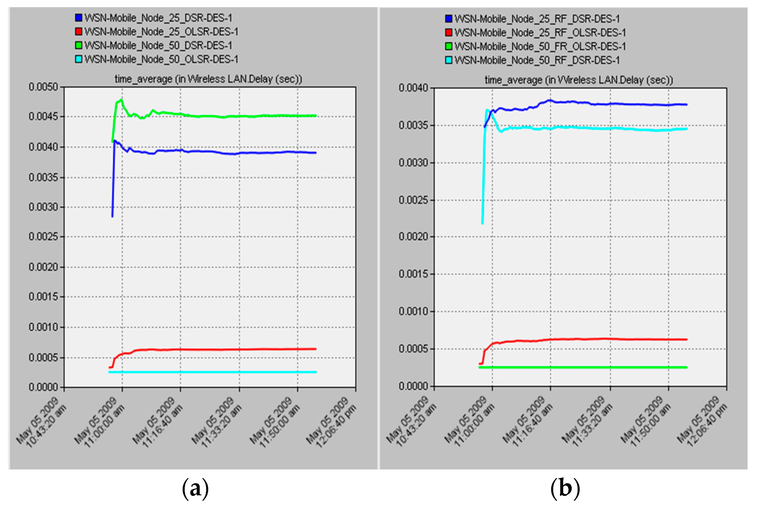
During the transmission phase of WLAN, the data (packets) are sent from the submitting nodes (senders) to the recipient nodes (receivers). The recipient nodes receive these data at their MAC layer, and they are then sent to higher levels. When we talk about end-to-end delay, we are referring to the amount of time it takes for an entire packet to be received at the WLAN MAC layer by all the nodes in the network and then transmitted to a higher layer. This encompasses the individual reception of all fragments and frames, transmission of frames through access point delay if enabled, and medium access delay at the source MAC.

Following the dissemination of this information, the proactive nature of the path toward every node ensures that it is always prepared, resulting in the lowest and most consistent delay. This indicates that there is no route discovery process in OLSR that is pre-computed, which guarantees the lowest possible latency, as Figure 3.

This is also demonstrated by the fact that the scenario with 50 nodes yields the same results for delay as the case with 25 nodes. This indicates that it performs well in vast networks, and the reason is, once again, the predetermined routing table entries for all of the nodes in the network. The amount of time needed to calculate the shortest path is not required, but the number of control messages will increase in large networks. In the instance of 50 nodes, not only did its rate drop to half of what it was at the beginning of the experiment, but it also took significantly more time to sustain a rate that was only marginally unstable. This suggests that the amount of time required for routing to reach all of the nodes and route maintenance will increase proportionally with the number of nodes in the network.

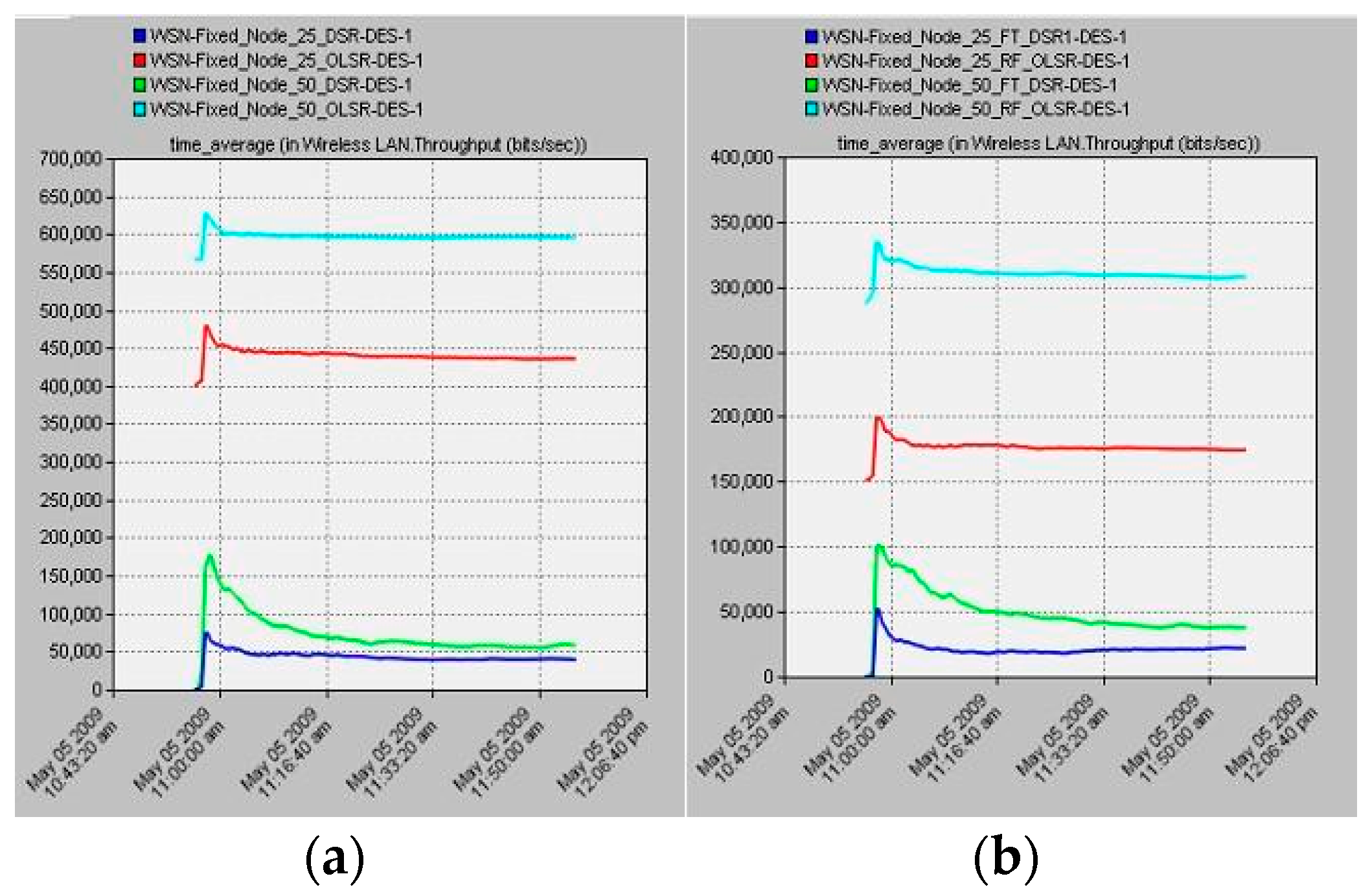
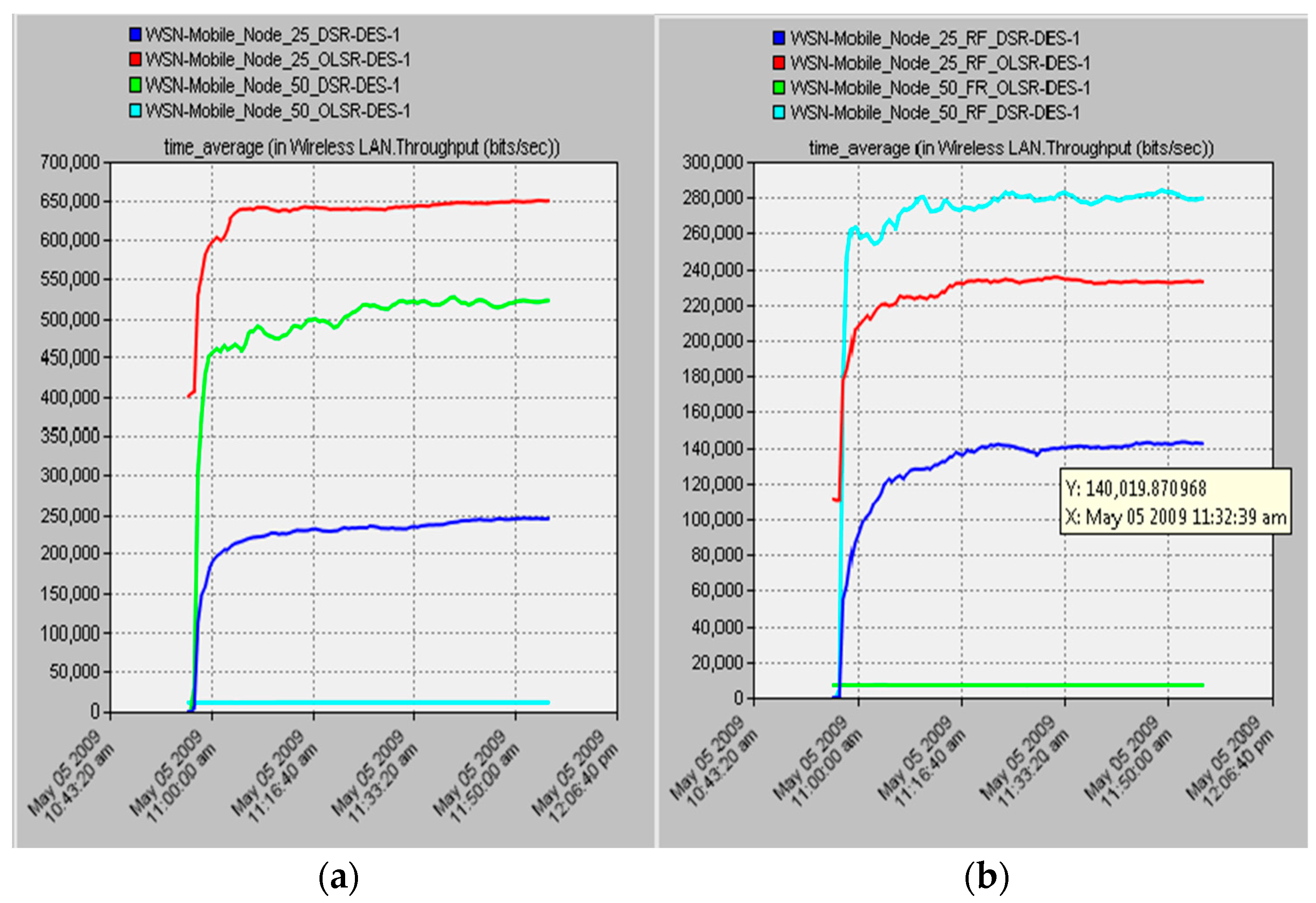
When looking at the node failure scenario for both 25 and 50 nodes, the 25-node scenario showed that the performance of DSR lowers from 50,000 bit/s to 20,000 bit/s, and in the 50-node scenario, it dropped significantly with a bigger ratio, from 100,000 bits/s to 40,000. This again suggests that the occurrence of random node failure will have a significantly more negative impact on densely populated networks in comparison to smaller networks. The reason for this is that when there are failed nodes present in a large network, it becomes extremely difficult to find a path from the source to the destination due to the consumption of resources (memory and energy), as well as the complexity of the overhead processes. On the other hand, if we take a look at the behavior of OLSR, we can see that it has a proactive routing nature, which results in the consistent nature of the routing overhead. This indicates that the paths to all of the nodes have already been calculated and established. The periodic updates of routing information are the sole overhead that is created at the network level, and their frequency is rather minimal. Even though the size of the network will have an impact on the routing overhead, it will still be reliable and consistent.

In both cases, the input parameters that were used were the same as those indicated in

Table 2. Parameter vs. Value for 2nd case.

Parameter	Value
Environment size	1000 × 1000 m
Number of nodes	25 and 50
Traffic type	Constant bit rate
Nodes type	Mobile
Packet rate	4 Packets/s
Packet size	512 byte
Number of Flows	25 and 50
Simulation time	3600 s
Number of submission hosts	25 and 50
Number of receivers	One

, with the exception of the number of nodes that were used. The outcomes of each statistic are depicted in Figure 4, Figure 5 and Figure 6 with regard to the various situations below.

4.3. End-to-End Delay

We will examine each scenario and compare both protocols with regard to the number of nodes and the kind of scenario in order to study the findings for end-to-end delay of the selected protocols in both scenarios with varied numbers of nodes. When we consider the scenario in Figure 4a, in which there is no failure of any of the nodes, we find that the DSR performs quite similarly whether there are 25 or 50 nodes present.

The availability of fewer alternate routes causes a lower increase in time in this case, but node mobility has no impact on the pattern of delay. The existence of numerous routes is the cause of this because it is evident from looking at the 50-node scenario that it provides a smaller delay with a constant rate.

There are few ROUTE ERROR messages and ROUTE REQUEST messages (route requests do not need to spread around the network). However, when a network expands, the proportion of ROUTE ERROR messages rises, which has an impact on the throughput rate, as evidenced by an unstable curve over time.

When compared to DSR, OLSR performs better in the case of 25 nodes, but as the network gets larger, it drastically reduces its rate. This is because of the way it operates. All paths are calculated in advance; however, because the nodes move around, its routing table entries are ineffective in larger networks. While it is possible to compute pathways at runtime in smaller networks, this is not viable in bigger networks, as Figure 7.

When examining the node failure scenario shown in Figure 5b, we can observe the throughput behavior of DSR in the 25-node example.

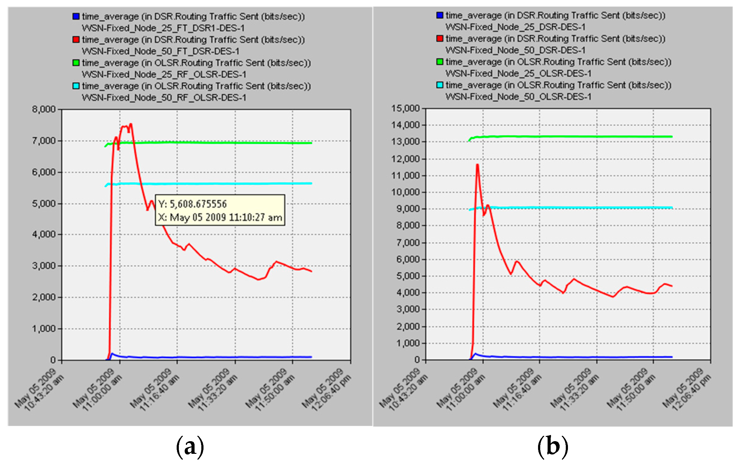
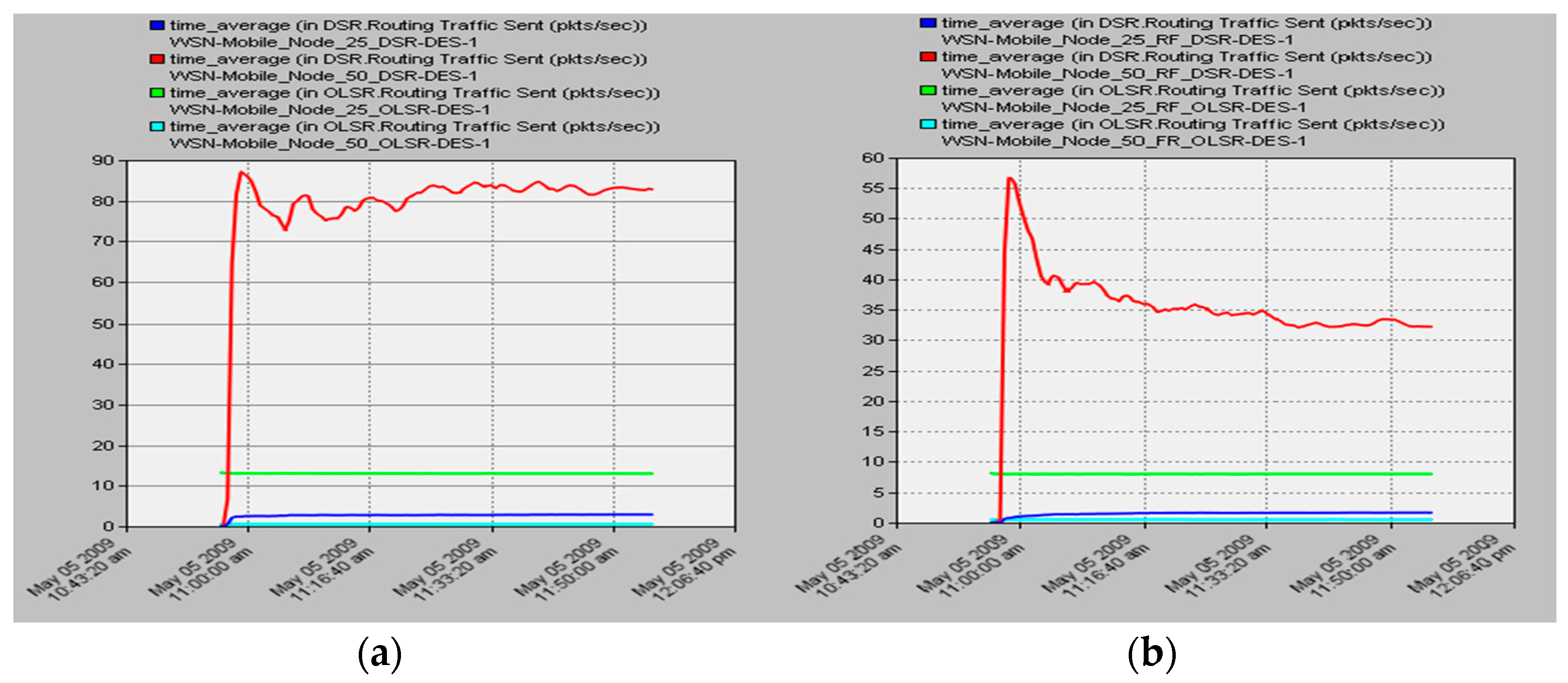
4.4. Routing Overhead

We will look at each scenario and compare both protocols with regard to the number of nodes and the kind of scenario in order to examine the findings for the routing overheads of DSR and OLSR in both scenarios with varied numbers of nodes. When we take into account the situation depicted in Figure 6a, which does not involve any nodes failing, we see that the DSR operates very differently in the case of 25 nodes compared to the case of 50 nodes. Because it uses source routing, the routing overhead for a smaller network, which consists of control messages, is low. This is also owing to the fact that it operates in a proactive manner. A ROUTE REQUEST message is sent whenever a route is required, and the ratio of ROUTE ERROR messages is low. However, as the size of the network expands, the routing overhead for the protocols that perform real-time routing (on time) undoubtedly increases. As a result, this caused a comparatively bigger overhead in the case of the 50-node scenario. When considering OLSR’s performance, it becomes immediately apparent that the protocol excels in both small and big networks. This is because it uses predetermined routes for each destination (node), which is why we have come to this conclusion. So, the only overhead that it shows are routing updates, topology control messages, and hello messages that are used to communicate that network, link, and node conditions have lowered after failure, which causes it to show a greater overhead to identify routes to different nodes. After a certain amount of time, the overhead continues to decrease due to a decrease in the number of executions of ROUTE REQUEST and ROUTE ERROR messages. Keeping route cache assists in overlooking the dead nodes, which in turn leaves retransmission to a higher tier.

In this paper, we have examined the simulated outcomes and performed some analyses on them. We ran simulations on wireless sensor networks with a variety of topologies and degrees of complexity and then reviewed the metrics obtained from those simulations. The primary metrics that have been taken into consideration throughout this paper are end-to-end delay, throughput, and routing overheads. We have simulated different network scenarios, including scalability and the failure of individual nodes, using both fixed and mobile node networks. For the purposes of the simulation, we have established specific parameters, and the results of the simulation have been displayed. In each of the test cases, the DSR and OLSR protocols were each given a separate implementation (simulation) so that their performance could be evaluated in relation to the proposed network in the context of scalability and the loss of nodes, as Figure 8.

5. Conclusions

The following is a conclusion that can be drawn based on the network type and routing challenges:

When it comes to delay, OLSR is more advantageous than DSR for both mobile and fixed nodes in a network. Additionally, node failure and network size do not have any significant effects on the performance of OLSR with regard to latency, but they do have such effects on DSR.

When it comes to throughput in networks with fixed nodes, OLSR outperforms DSR in both small and big networks, and a failed node has a much smaller impact on OLSR than it does on DSR. However, in mobile node networks, OLSR performs better for small networks, while DSR performs well for large networks. Additionally, the effect of a node failure affects the network in a different way depending on the size of the network; specifically, the influence on DSR is smaller in large networks, while the effect on OLSR is lesser in small networks.