A Python Module for Implementing Cointegration Tests with Multiple Endogenous Structural Breaks ^†

Abstract

Testing for long-run relationships between time series variables with short-run adjustments is an integral part of many empirical studies nowadays. Allowing for structural breaks in the estimations is a pertinent issue within this context. The purpose of this paper is to provide a consumer-friendly module that is created in Python for implementing three residuals-based cointegration tests with two unknown regime shifts. The timing of each shift is revealed endogenously. The software is easy to use via a Graphical User Interface (GUI). In addition to implementing cointegration tests, the software also estimates the underlying parameters along with the standard errors and the significance tests for the parameters. An application is also provided using real data to demonstrate how the software can be used. To our best knowledge, this is the first software component created in Python that implements cointegration tests with structural breaks.

1. Introduction

Cointegration analysis is an integral part of the tool kit for empirical analyses of time series data. The idea was introduced by Granger [1]. Testing for cointegration is an important issue because if the variables in a regression model have a unit root but the linear combination is not stationary, then the underlying regression relationship is spurious. However, if the linear relationship is stationary, it means the variables have a joint stochastic trend that cancel each other out in the long run, and the resulting relationship is genuine. It is also possible to combine the long-run relationship with the short-run adjustment when testing for cointegration. Tests for cointegration were developed by, among others, Engle and Granger [2], Johansen [3], Johansen and Juselius [4], Phillips [5], Phillips and Ouliaris [6], and Stock and Watson [7]. The next classes of tests for cointegration account for potential structural breaks that can take place during the sample period. These structural breaks can be caused by a number of factors such as tectological progress, organizational evolution, financial crises, natural crises, conflicts, and so on. Accounting for structural breaks when tests for cointegration are conducted not only results in more informative empirical findings but also increases the precision of the underlying inference since tests for cointegration have lower power if the impact of significant structural breaks is not taken into account. Standard tests for cointegration have low power if there are structural breaks during the sample period but are disregarded in the estimations. There are several logical reasons behind structural breaks (such as technological advancements, natural catastrophes, human-made catastrophes, organizational evolutions, or system modifications, among others). Gregory and Hansen [8] introduced three residual-based tests for cointegration that account for one unknown structural break. Hatemi-J [9] developed three tests for cointegration that account for two unknown regime shifts. The purpose of this work is to introduce a software component written in Python (https://www.python.org/) to implement these tests with two unknown regime shifts. To our best knowledge, statistical software components for implementing these cointegration tests are missing in Python, which is an open-source program. Thus, the objective of the current article is to introduce and demonstrate a module created by the authors in Python for implementing three residual-based tests of Hatemi-J [9] for cointegration. The module is consumer-friendly, and it can easily be utilized via a Graphical User Interface (GUI). It should be mentioned that a procedure for implementing these tests in Gauss was developed by Aptech Systems [10]. The Gauss code created by Hatemi-J [11] is also available online.

The rest of this article is organized as follows. In Section 2, an example is provided to demonstrate how cointegration can take place between two variables that have a unit root each. Section 3 presents the test methods that can be used for testing for cointegration with two unknown regime shifts. Section 4 describes the software component that is created in Python and presents the estimation results. The Section 5 offers conclusions.

2. A Simple Example of Cointegration

In this example, we demonstrate explicitly when cointegration takes place between two variables that each have one unit root or are integrated in the first order, denoted by I(1). Observe two I(1) variables that have the following data-generating process (DGP):

$$V_t=V_{t-1}+{\epsilon }_{1,t}$$

(1)

$$W_t=V_{t-1}+{\epsilon }_{2,t}$$

(2)

Here, ${\epsilon }_{1,t}$ and ${\epsilon }_{2,t}$ represent two IID (independent and identically distributed) error terms. Suppose that the initial value is zero in each case; by using the continuous substitutions method, each variable has the following solution:

$$V_t={\displaystyle \sum }_{j=1}^t {\epsilon }_{1,j}$$

(3)

$$W_t={\displaystyle \sum }_{j=1}^{t-1}{\epsilon }_{1,j}+{\epsilon }_{2,t}$$

(4)

Next, obtain the change in each variable as below:

$$\Delta V_t=V_t-V_{t-1}={\displaystyle \sum }_{j=1}^t{\epsilon }_{1,j}-{\displaystyle \sum }_{j=1}^{t-1}{\epsilon }_{1,j}={\epsilon }_{1,t}$$

(5)

$$\Delta W_t=W_t-W_{it-1}={\displaystyle \sum }_{j=1}^t{\epsilon }_{i1,j}+{\epsilon }_{i2,t}-\left({\displaystyle \sum }_{j=1}^{t-1}{\epsilon }_{i1,j}+{\epsilon }_{i2,t-1}\right)={\epsilon }_{i1,t}+{\epsilon }_{i2,t}-{\epsilon }_{i2,t-1}$$

(6)

The symbol $\Delta$ is representing the first difference operator. Thus, each I(1) time series converts to a stationary process in the first difference format. An important question within this context is whether these two I(1) variables are cointegrated or not. Let K_t represent the difference between V_t and W_t. Therefore, we have the following result:

$$K_t=W_t-V_t={\displaystyle \sum }_{j=1}^t{\epsilon }_{1,j}-\left({\displaystyle \sum }_{j=1}^{t-1}{\epsilon }_{1,j}+{\epsilon }_{2,t}\right)={\epsilon }_{1,t}-{\epsilon }_{2,t}$$

(7)

The difference defined above is evidently a stationary process. A linear relationship between the two integrated processes is stationary. The implication of this outcome is that V_t and W_t are cointegrating and their cointegrating vector is (1.00, −1.00) in this case. It is important to notice that the reason for the variables V_t and W_t cointegrating is the fact that they have a joint stochastic trend in the long run that cancels each other out. That is why cointegration takes place in this particular case (for more on unit roots and cointegration inference, see Hatemi-J [12,13]).

3. Tests for Cointegration with Two Structural Breaks

Consider the following model that is considered for application in an empirical study using time series data:

$$y_t={\alpha }_0+{\alpha }_1{D}_{1t}+{\alpha }_2{D}_{2t}+{\beta }_0{x}_t+{\beta }_1{D}_{1t}{x}_t+{\beta }_2{D}_{2t}{x}_t+u_t$$

(8)

where y_t is the dependent variable and x_t is a vector of the independent variables. The parameter ${\alpha }_0$ is the intercept, ${\alpha }_1$ is the first change, and ${\alpha }_2$ is the second change in the intercept. The vector ${\beta }_0$ represents the slopes. ${\beta }_1$ is the first change and ${\beta }_2$ is the second change in the slope vector. D_1t and D_2t are dummy variables that are identified as

$$D_{1t}=\left\{\begin{array}{c}0,\hspace{1em}if t\le \left[n{\tau }_1\right]\\ 1,\hspace{1em}if t>\left[n{\tau }_1\right]\end{array}\right.$$

(9)

$$D_{2t}=\left\{\begin{array}{c}0,\hspace{1em}if t\le \left[n{\tau }_2\right]\\ 1,\hspace{1em}if t>\left[n{\tau }_2\right]\end{array}\right.$$

(10)

with the unknown parameters ${\tau }_1$ ∈ (0, 1) and ${\tau }_2$ ∈ (0, 1) signifying the relative timing of each structural break.

To test for the null hypothesis of no cointegration in the presence of two unknown regime shifts, the following regression can be estimated:

$$\Delta {\widehat{u}}_t={\gamma }_0+\rho {\widehat{u}}_{t-1}+{\displaystyle \sum }_{l=1}^L{\mathrm{c}}_l\Delta {\widehat{u}}_{t-l}+e_t$$

(11)

where ${\widehat{u}}_t$ represents the estimated error term via the ordinary least squares (OLS) method. The lag order L needs to be determined by minimizing an information criterion. For more information on the selection of optimal lag orders in a dynamic model, see Hatemi-J [14], Hacker and Hatemi-J [15], and Mustafa and Hatemi-J [16]. There are three test methods that can be used for this purpose. The first one is the modified augmented Dickey–Fuller (ADF) [17] test statistic that is estimated as the following:

$$ADF=\frac{\widehat{\rho }}{SE\left(\widehat{\rho }\right)}$$

(12)

where $\widehat{\rho }$ is the estimated value of $\rho$ and $SE\left(\widehat{\rho }\right)$ represents its standard error. The other two test methods are the modified tests of Phillips and Ouliaris [6] denoted as $Z_{\alpha }$ and $Z_t$. These tests are defined as

$$Z_{\alpha }=n\left({\widehat{\rho }}^{*}-1\right)$$

(13)

and

$$Z_t=\frac{\left({\widehat{\rho }}^{*}-1\right)}{\left(\widehat{\gamma }\left(0\right)+2{{\displaystyle \sum }}_{j=1}^B\omega \left(j/B\right)\widehat{\gamma }\left(j\right)\right)/{{\displaystyle \sum }}_1^{n-1}{\widehat{u}}_t^2}$$

(14)

where

$${\widehat{\rho }}^{*}=\frac{{{\displaystyle \sum }}_{t=1}^{n-1}\left({\widehat{u}}_t{\widehat{u}}_{t+1}-{{\displaystyle \sum }}_{j=1}^B\omega \left(j/B\right)\widehat{\gamma }\left(j\right)\right)}{{{\displaystyle \sum }}_{t=1}^{n-1}{\widehat{u}}_t^2}$$

(15)

and

$$\widehat{\gamma }\left(j\right)=\frac{1}{n}{\displaystyle \sum }_{t=j+1}^T\left({\widehat{u}}_{t-j}-\widehat{\rho }{\widehat{u}}_{t-j-1}\right)\left({\widehat{u}}_t-\widehat{\rho }{\widehat{u}}_{t-1}\right)$$

(16)

Hatemi-J [9] suggests finding the optimal test values with two unknown structural breaks as the following:

$$AD{F}^{*}=\underset{\left({\tau }_1,{\tau }_2\right)\in T}{\inf }ADF\left({\tau }_1,{\tau }_2\right)$$

(17)

$$Z_t^{*}=\underset{\left({\tau }_1,{\tau }_2\right)\in T}{\inf }{Z}_t\left({\tau }_1,{\tau }_2\right)$$

(18)

$$Z_{\alpha }^{*}=\underset{\left({\tau }_1,{\tau }_2\right)\in T}{\inf }{Z}_{\alpha }\left({\tau }_1,{\tau }_2\right)$$

(19)

These tests have non-standard distributions. Hatemi-J [9] created critical values using simulations and the surface response method. The size and power properties of these modified tests are also investigated by the mentioned author, which shows that the tests have an accurate size and much higher power accuracy compared to the standard tests.

4. The Phyton Module

In this section, our module created in Python for estimating the tests for cointegration with two regime shifts is presented.

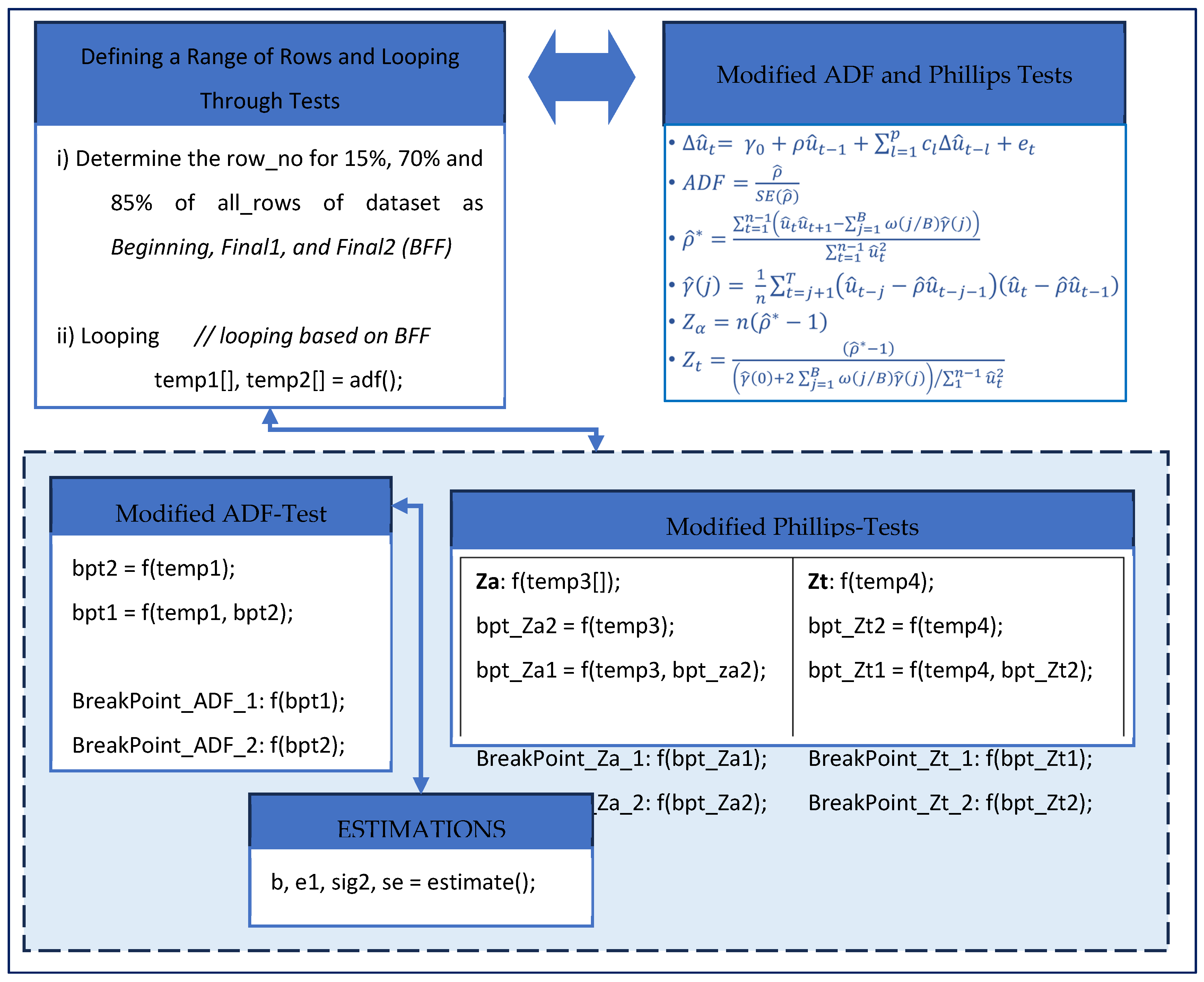
4.1. Pseudocode for the Module

The module comprises five major sections. The overall structure of the module which controls the flow of data between the sub-sections of the module is entitled “Defining a range of rows and looping through tests”, with the collection of mathematical rules being stored in the “ADF and Philips Tests” section, and both tests of “Modified ADF-Test” and “Modified Phillips-Tests” will calculate their different methods used and backed by the mathematical algorithms designed in the earlier section. The last sub-section is named “Estimations”, which provides a series of estimated values to support the calculation of “Modified ADF-Test”. A view of this pseudocode is provided in Figure 1.

4.2. The Graphical User Interface and a Numerical Application

Figure 2 shows a Graphical User Interface (GUI) for the module to help interact with the algorithms designed in this research. The data were collected from the Bloomberg database. Two indices were used for gold and the World Stock Price Index covering periods of [1 February 2018] until [25 May 2023]. The number of observations is 1404. Each variable is transformed to natural logarithmic values before entering them into the module. Thus, each estimated slope represents elasticity. The Python code that is used for conducting the estimations is produced by [18], which is available online.

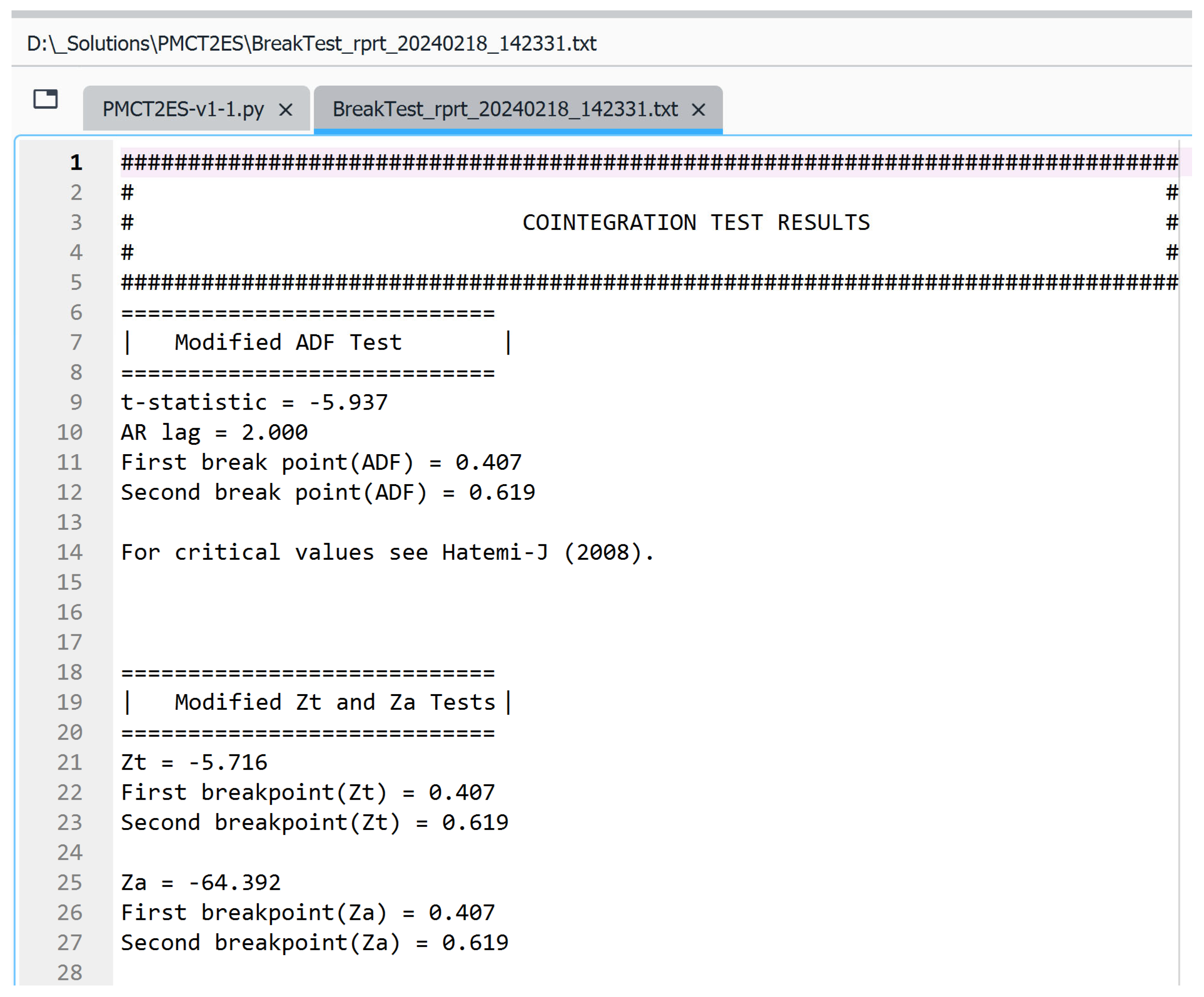
4.3. Outputs of the Module

Several outputs are created by the module to provide the user with accessibility to the outcome of the process, as shown in Figure 3.

In Figure 3, the estimation results of all three tests are provided along with the timing of each unknown structural break. The estimated value of each test needs to be compared to the critical values provided by Hatemi-J [9] (Table 1 on page 501). In this particular case, in which we have only one independent variable in the model, the critical values for the modified ADF-Test and the modified $Z_{\alpha }$ test are −6.503, −6.015, and −5.653 at the 1%, 5%, and 10% significance levels, respectively. The critical values for the modified $Z_t$ test are −90.794, −76.003, and −52.232, respectively. Thus, the null hypothesis of no cointegration, against the alternative hypothesis of cointegration in the presence of two regime shifts, can be rejected at the 10% significance level only by each test. Via multiplying the value of each break by the number of observations, the exact timing of each break can be determined. Thus, the first structural break takes place at observation 572 (i.e., 0.407 × 1404), which corresponds to 11 March 2020. Similarly, the second break occurs at observation 870 (i.e., 0.619 × 1404), which corresponds to 4 May 2021.

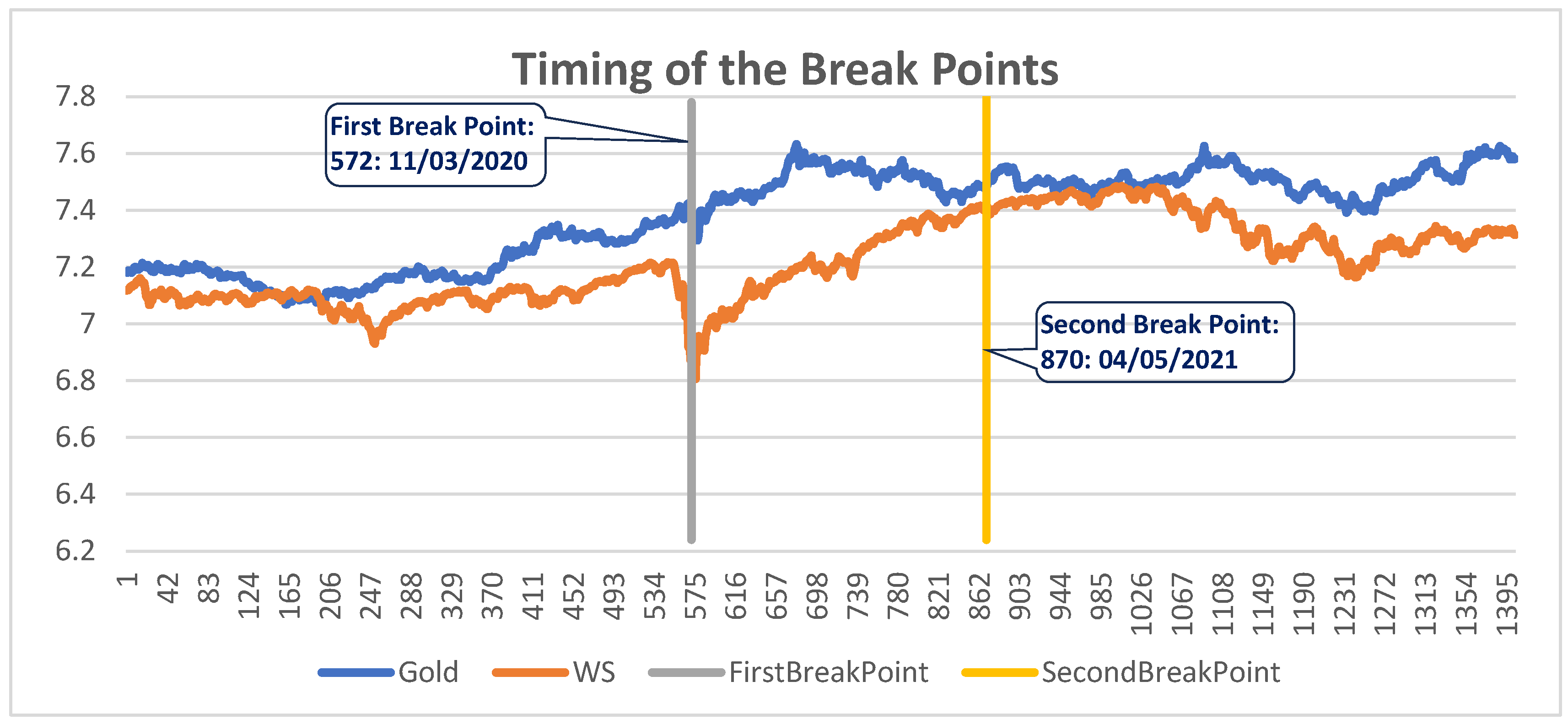
4.4. Chart Created Based on the Output of the Module

As part of the visual presentation of the outcome, it is commonly known that charts can present a better clarification of how data stand, as demonstrated in Figure 4.

Based on the estimation results presented in Figure 3 in the previous sub-section, the first structural break took place on 11 March 2020 and the second break occurred on 4 May 2021. These results seem to depict the three regimes that took place before, during, and after the COVID-19 pandemic.

The estimation results of the underlying parameters are presented in

Table 1. Estimation results.

Parameters	Estimated Parameters	Standard Errors	t-Statistics
${\alpha }_0$	1.345052	0.356620	3.771663
${\alpha }_1$	4.784411	0.403131	11.868144
${\alpha }_2$	0.510514	0.298069	1.712736
${\beta }_0$	0.825965	0.050246	16.438452
${\beta }_1$	−0.636381	0.056591	−11.245172
${\beta }_2$	−0.071286	0.040834	−1.745746

, which show that there are two significant shifts in both the intercept and the slope. Based on these results, it can be concluded that the stock prices in the world market have a positive effect on gold prices. If the stock prices increase by 1%, then the gold prices will increase by 0.825965%, ceteris paribus. However, this value decreases by 0.636381% during the pandemic period, and it decreases by 0.071286% for the period after the pandemic.

5. Conclusions

Implementing tests for cointegration when time series data are used in empirical investigations is important to avoid the spurious regression problem. Allowing for structural breaks improves the inference. This work introduced our software component created in Python for this purpose. To our best knowledge, this is the first attempt to provide an open-source software component that implements tests for cointegration with two unknown structural breaks. The timing of each break is determined by the software component endogenously. The software uses a Graphical User Interface, which makes its operation straightforward. The software also estimates the unknown timing of each break and the parameters. A numerical application is provided in order to demonstrate step-by-step how the software can be utilized and how the estimation output can be interpreted by practitioners.

References

1. Granger, C.W. Some properties of time series data and their use in econometric model specification. J. Econom. 1981, 16, 121–130. [Google Scholar] [CrossRef]
2. Engle, R.; Granger, C.W. Cointegration and error correction: Representation, estimation and testing. Econometrica 1987, 35, 251–276. [Google Scholar] [CrossRef]
3. Johansen, S. Statistical analysis of cointegration vectors. J. Econ. Dyn. Control 1988, 12, 231–254. [Google Scholar] [CrossRef]
4. Johansen, S.; Juselius, K. Maximum likelihood estimation and inference on cointegration—With applications to the demand for money. Oxf. Bull. Econ. Stat. 1990, 52, 169–210. [Google Scholar] [CrossRef]
5. Phillips, P.C. Time series regression with a unit root. Econometrica 1987, 5, 277–301. [Google Scholar] [CrossRef]
6. Phillips, P.C.; Ouliaris, S. Asymptotic properties of residual based tests for cointegration. Econometrica 1990, 58, 165–193. [Google Scholar] [CrossRef]
7. Stock, J.H.; Watson, M.W. Testing for common trends. J. Am. Stat. Assoc. 1988, 83, 1097–1107. [Google Scholar] [CrossRef]
8. Gregory, A.W.; Hansen, B.E. Residual-based tests for cointegration in models with regime shifts. J. Econom. 1996, 70, 99–126. [Google Scholar] [CrossRef]
9. Hatemi-J, A. Tests for cointegration with two unknown regime shifts with an application to financial market integration. Empir. Econ. 2008, 35, 497–505. [Google Scholar] [CrossRef]
10. Aptech Systems. GAUSS Platform. 2024. Available online: https://www.aptech.com/ (accessed on 10 January 2024).
11. Hatemi-J, A. CItest2b: GAUSS Module to Implement Tests for Cointegration with Two Unknown Structural Breaks, Statistical Software Components G00006, Boston College Department of Economics. 2009. Available online: https://ideas.repec.org/c/boc/bocode/g00006.html (accessed on 5 February 2023).
12. Hatemi-J, A. Essays on the Use of VAR Models in Macroeconomics. Ph.D. Thesis, Econometrics, Department of Economics, Lund University, Lund, Sweden, 1999. [Google Scholar]
13. Hatemi-J, A. Time-Series Econometrics Applied to Macroeconomic Issues. Ph.D. Thesis, Internationella Handelshögskolan, Jonkoping University, Jönköping, Sweden, 2001. [Google Scholar]
14. Hatemi-J, A. A new method to choose optimal lag order in stable and unstable VAR models. Appl. Econ. Lett. 2003, 10, 135–137. [Google Scholar] [CrossRef]
15. Hacker, R.; Hatemi-J, A. Optimal lag-length choice in stable and unstable VAR models under situations of homoscedasticity and ARCH. J. Appl. Stat. 2008, 35, 601–615. [Google Scholar] [CrossRef]
16. Mustafa, A.; Hatemi-J, A. A VBA module simulation for finding optimal lag order in time series models and its use on teaching financial data computation. Appl. Comput. Inform. 2022, 18, 208–220. [Google Scholar] [CrossRef]
17. Dickey, D.A.; Fuller, W.A. Distribution of the estimators for autoregressive time series with a unit root. J. Am. Stat. Assoc. 1979, 74, 427–431. [Google Scholar]
18. Mustafa, A.; Hatemi-J, A. PMCT2ES: Python Module for Cointegration Tests with Two Endogenous Structural Shifts. Statistical Software Components, Nr. P00002, Boston College Department of Economics. 2022. Available online: https://ideas.repec.org/c/boc/bocode/p00002.html (accessed on 21 March 2024).
Figure 1. A view of the pseudocode for the PMCT2ES Module.
Engproc 68 00010 g001
Figure 2. A snapshot of the Graphical User Interface used to ease the process of data entry and generate outputs to/from the system [9].
Engproc 68 00010 g002
Figure 3. One of formats of output generated by the module in a text format [9].
Engproc 68 00010 g003
Figure 4. A view of data output for both break points in the form of a chart for both gold and World Stock Price Index.
Engproc 68 00010 g004