Abstract
Coupling a reservoir neural network and a Grey Wolf optimization algorithm the system hyperparameters space is explored to find the configuration best suited to forecast the input sensor from the NASA CMAPSS dataset. In such a framework, the application to the problem of predictive maintenance is considered. The necessary requirements for the system to generate satisfactory predictions are established, with specific suggestions as to how a forecast can be improved through reservoir computing. The obtained results are used to determine certain common rules that improve the quality of the predictions and focus the optimization towards hyperparameter solutions that may allow for a faster approach to predictive maintenance. This research is a starting point to develop methods that could inform accurately on the remaining useful life of a component in aerospace systems.
1. Introduction
Experience is the foundation for any modern maintenance process. Thus all prognostics on complicated systems are either model-based or data-driven. The former depends on the use of physics-based models of the degradation processes and are typically applied to safety-critical and slow-degrading equipment whose degradation mechanisms have been extensively studied. The latter, only used when no accurate physics model is available, requires enormous amounts of data for training, only being applied to non-safety critical systems with short mean time to failure [1].
Model-based prognostics have been the preferred choice during the last century, resting the required actions to be taken as much from the physical knowledge behind the model as from the experience of the engineers tasked to maintain it. At the dawn of this millennia though, new technologies originated providing a far more powerful process to predict failure of a mechanical system given enough data on it. The advent of Machine Learning brought a whole new set of tools to predict, simulate and diagnose events that would be catastrophic if occurring on a real-life scenario, allowing an increase in reliability across all modern industrial fields.
Data-driven models are therefore gaining significant traction in the engineering landscape, specially in Aerospace, as even reduced improvements through computing-intensive simulations can yield millions through efficiency savings on the long run. Not only Machine Learning is being used extensively, but digital models are being widely employed so as to combine both technologies and speed up greatly project development. Industrial applicability of data-driven frameworks [2] have been prominently favored by causes as: the increase in data availability; high performance computing; improved data storage and sensor technologies and a greater academic focus on algorithms and applied mathematics; not to mention a flood of investment.
Predictive maintenance is also gaining traction through the combination of increased capabilities in sensor networks as well as computational power. The ability to pour through high dimensional and multivariate data and classify its internal relationships is key to determine the potential failures bound to happen [3].
The advantages of using Reservoir Neural Networks Computing (RC from now on) for predictive maintenance in aerospace have been explored before, especially on components with easy to acquire data, e.g.,: to predict medium and long-term fluctuations on avionic modules with an Echo State Network (ESN) [4], allowing for preventive maintenance in case it strides off from its nominal value; or using an ESN to predict the Remaining Useful Life from the operational data of several turbofan engines, analysing operational settings and sensor information to determine how many cycles are left before catastrophic failure [5].
Accurate signal prediction opens up the door for efficient and safe control, automatically adjusting and correcting any kind of output sensor whether the operational settings (OP) of an engine, the flight-path of a drone, the coordination of a bipedal robot or human controlled situations [6]. If fully integrated into a system, it will prevent from failures caused by sluggish control algorithms that simply react once the action has happened, rather than adjusting the system to prevent it.
2. Materials and Methods
2.1. RC-GWO System
In this work we report the construction of an hybrid system involving the coupling of a reservoir neural network and a Grey Wolf optimization algorithm which we will call the Reservoir Computing-Grey Wolf Optimizer system (RC-GWO from now on). Such a system receives an input composed by sensor signals and explores the hyperparameter space to find the configuration best suited for a specific prediction. Once the system finds the optimal settings for a reservoir it is not necessary to run it again for generating new predictions of an updated dataset. For instance, let us consider the example of the power consumption of a device during three years, the training data could be selected to be all available data apart form the last two months and the validation data those last two months. When the appropriate reservoir hyperparameters configuration has been found, new results could be quickly generated bimonthly without having to optimize the neural network. This can be repeated until the normalizedmean square error of the predictions differs from a given tolerance and the process begins anew. To optimize the reservoir certain hyperparameters must be defined. Ref. [7] serves as a foundation for defining the optimal configuration vector which the wolves will try to hunt down.
2.1.1. Reservoir Computing
RC is a specific type of Recurrent Neural Network (RNN) consisting of two components: a nonlinear dynamical system that accepts an input signal (the reservoir) and one trainable layer (called the readout layer) producing the output. If the reservoir is complex enough, in principle, any computation can be achieved by just training the readout layer to achieve a desired functionality [8]. This approach was first introduced in [9,10], using the terms Echo State Networks (ESN) and Liquid State Machines (LSM) but nowadays it is better known by the general term reservoir computing (RC), to stress the role of the reservoir but also to make a difference with Liquid Neural Nets (LNNs) [11]. RC has been shown to be particularly useful to handle chaotic time-series prediction and other complex tasks effectively [12].
A reservoir can be composed by a random combination of activation functions that is capable of encoding the original dynamics into higher dimensions. Any system can be considered a reservoir given an input, an output and an interpretation layer transforming the output into readable information. Take for instance the use of Brain Organoids—brain-like 3D in vitro cultures—as a reservoir due to its capacity for nonlinear dynamics and fading memory properties [13]. In the case of RC the relationships between the elements of the reservoir (neurons characterized by an activation function) define a graph given by an adjacency matrix. Given an input the resulting state of an activation function promote specific paths for the propagation of the stimulus. Training a reservoir is nothing but observing during enough time how it reacts to a given set of information and making a linear correlation with a desired output, not delving in the complex dynamics that develops inside and only skimming the surface reaction for answers.
The reservoir employed on the RC-GWO system is based on the ESN, which establishes the required mathematical properties of a valid reservoir through the Echo State Property (ESP). A good reservoir is one that is able to separate inputs; different external inputs should drive the system to different regions of the configuration space. This is called the separability condition [14], which relates asymptotic properties of the excited reservoir dynamics to the driving signal. Intuitively, the ESP states that the reservoir will asymptotically wash out any information from initial conditions. The ESP is guaranteed for additive-sigmoid neuron reservoirs, if the reservoir weight matrix (and the leaking rates) satisfy certain algebraic conditions in terms of singular values. For such reservoirs with a tanh sigmoid, the ESP is violated for zero input if the spectral radius of the reservoir weight matrix is larger than unity. Conversely, it is empirically observed that the ESP is granted for any input if this spectral radius is smaller than unity. This has led to a far-spread but erroneous identification of the ESP with a spectral radius below 1. Specifically, the larger the input amplitude, the further above unity the spectral radius may be while still obtaining the ESP [15]. For a reservoir to hold the ESP it must resonate information of all the inputs through the consequent internal states.
Given an N neurons reservoir, their links strength (weights) are represented by an matrix, , with values selected from an uniform random distribution in the interval . Therefore the reservoir is described by . Let’s consider an input vector containing the sensor time series, with . This input sensor data is introduced into the reservoir by means of an input-reservoir coupler, i.e., a randomly generated matrix, , whose elements are drawn from an uniform random distribution in the interval , i.e., it is generated as in the case for , but all elements of should be non-zero, additionally, does not require normalization.
Once and have been set up, the internal states for each of the inputs are harvested. Typically the neurons used for this reservoir are discrete-time leaky-integrate units, ruled by the update equations:
where, is the vector with the internal states of neurons in the reservoir, is its update vector for new inputs, all at time step t, is the leaking rate and is the vertically concatenated unitary value with the input at time step t. Then the network output, , is given by:
The computation of is a linear equation system. It is fixed by means of a ridge-regression, also known as Tikhonov regularization:
where, , is the internal states matrix in which the columns are state vectors , for ; is the output objective used for training, is the output weight matrix needed to interpret the internal states back to a usable output, is the identity matrix and is the regularization coefficient. Once the training is finished, the internal states have been harvested and the ridge-regression applied, the prediction phase runs on Equations (1)–(3), where the input is the predicted output of the preceding step .
2.1.2. Grey Wolf Optimizer
The Grey Wolf Optimizer (GWO) is a meta-heuristic method proposed by Mirjalili et al. [16], based on the hunting patterns of grey wolves, mimicking their leadership hierarchy and hunting procedures. It is based on the fact that wolves have a rigid social structure, with a lead individual, known as alpha, making the decisions. It comes followed by the beta wolf, which enforces the alphas’ decisions and gives feedback. The omega wolf is the lowliest of all, being the last to eat and basically acting as an scapegoat to prevent infighting.
The main phases of grey wolf hunting are: tracking, chasing and approaching prey; pursuing, encircling and harassing the prey until it stops moving; and attacking towards the prey. A mathematical model of this collective behaviour is what drives the optimization algorithm, candidates sharing information about the drive space, assisting in avoiding locally optimal solutions and exploring the objective space.
The first step is to establish that the fittest solution is the wolf, followed respectively by the and . Whatever remains of the population at that point are considered wolves, and follow the three lead wolves. The motion of wolves is described as:
Here, t, is the discrete iteration, and random vectors, the position of the prey and the position of the wolves, and:
with, decreasing linearly from to over the course of the iterations until the maximum number of them, T, is reached. As in the original algorithm only its initial and final value are specified, for the sake of simplicity it is usual to set to a scalar, e.g., so that a decrease linearly from 2 to 0. , and are random vectors uniformly distributed in , and are of a dimension matching that of the wolves position vectors.
To hunt for the prey we need the location of the optimum, unfortunately this is an unknown. To simulate the hunting behaviour [16], the , and wolves are believed to have the most information on where that optimum is. Whenever a new population needs to be spawned, the three lead wolves are taken as a reference and the rest are forced to update their positions accordingly. In this process the distance between the , and wolves and the prey is modeled as:
where , and are the locations of leading wolves; , and represent random vectors, and specifies the location of the present solution. The estimation of the distances allows for the update rules:
and,
where , and are random vectors and t is the recent iteration. The parameter a as given by (10) is modelled to signify the end of the hunt once the prey stops moving. The norm of fluctuates in the interval , where the elements of a are linearly decreased from 2 to 0. To promote exploration may take different values; —as just mentioned—focuses the wolves on the hunt, , drives them to diverge from the prey and to find a better solution. The random vector also plays part in the optimization exploration phase [16]: when , it encourages exploration while for , de-emphasizes it. In particular, the exploitation trend improves for and . Thus, provides random weights for the prey term in order to stochastically promote () or impede () the effect of prey in defining the distance in (6); opposite to , does not linearly decrease with a in order to always enforce exploration.
The algorithm has been altered with respect to [16], as in our case some parameter bounds need to be established during the exploration phase. When a new population is generated their location are required to be within bounds. If wolves are not within bounds, the generation is repeated again and again until they are. Testing has proven that in some edge situations, a new population is always out of bounds. When that happens a countdown is activated, and once a wolf has been repopulated a certain amount of times the out of bounds coordinates in the exploration space are changed by a random value within the space defined by the three lead wolves. Such a procedure allows for exploration while guaranteeing wolves will not remain stuck in an out of bounds position.
2.1.3. System Architecture
The RC-GWO system, receives an input signal and runs through the hyperparameter space to find the best suited configuration for an specific prediction. Once the system finds optimal settings for a reservoir it is not needed to run it again to generate new predictions for an updated dataset. To optimize the configuration of a reservoir a set of hyperparameters must be defined. Ref. [7] serves as a foundation for defining the optimal configuration. Once , and , are generated—as explained above—the following reservoir parameters are needed: (1) The size of the reservoir, N. It is fundamental to appropriately capture the inherent complexity of the input sensor time series. As a rule of thumb, the more challenging the task the bigger the reservoir should be. Some limitations should be established to avoid overfitting and to avoid unnecessary computations. (2) The leak rate, . It represents the speed of the reservoir update dynamics discretized in time. The closer to 1 the more it will forget about the previous internal states the reservoir went through. (3) The input matrix column scaling factor, . It needs to be as many as different inputs are ingested in the reservoir, always being at least two for the present ensemble. Each of the scaling factors apply to a specific column of the input weight matrix, with the first always being the one for the unitary value that accompanies the input and from the second onward for the input itself. In case the input sensor data is more than a single time series it is recommended to group them and apply the same factor for those that contribute differently to the task. (4) The sparsity of the reservoir, c. It represents the connectivity among the neurons in the reservoir. In [7] it is stated that when connecting each reservoir node to a small number of other nodes (e.g., 10) on average, irrespective of the reservoir size, computation speeds up. Sparse matrix representations are recommended as they give slightly better performance, but in general this hyperparameter does not affect much the quality of the prediction. As indicated in [15], some authors have developed fully connected reservoirs which work as well as sparsely connected ones. (5) The spectral radius scaling factor, . It is used to enforce the echo state property through establishing the maximal absolute eigenvalue of the internal weight matrix, . Once a random sparse matrix is generated, its spectral radius, , is computed. Then is divided by the spectral radius to yield a matrix with unitary spectral radius and scaled with to adapt to the specific input ingested in the reservoir, i.e.,
(6) The last hyperparameter to be tuned is the Tikhonov regularization coefficient, , which serves to obtain the output layer through ridge-regression. A matrix with high values is an indication of a very sensitive and unstable solution.
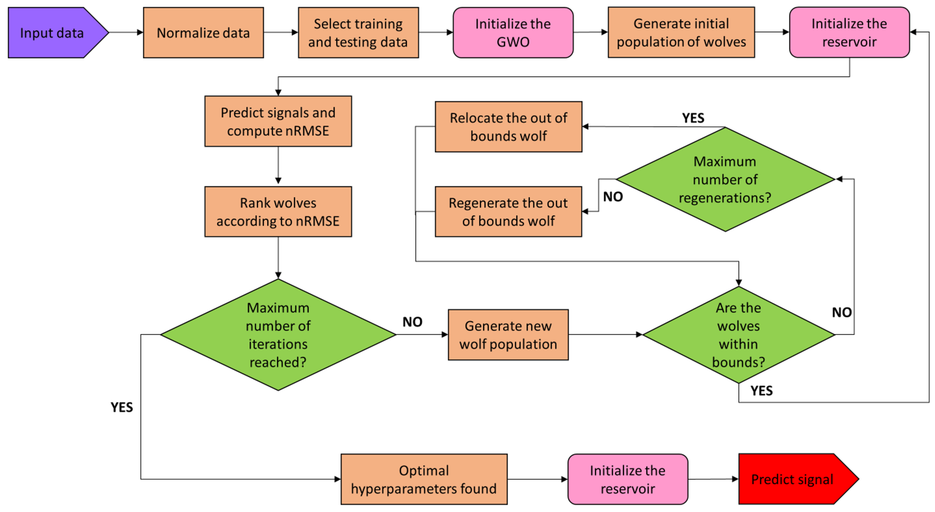
Once the ensemble is initialized it will determine autonomously the best suited set of hyperparameters for a given input sensor data with minor tweaking necessary. Figure 1 shows the system workflow. The GWO algorithm is called and then the reservoir runs for evaluating the wolves. Once the data is ingested the normalized sensor data is calculated,
where is the sensor data at t, and and are the mean and standard deviation. The data needs is normalized, to guarantee the outliers do not “squash out” the rest of the data when applied to the activation function.

Figure 1.
RC-GWO system flowchart. The sensor data enters as an input for pre-processing and hyperparameters optimization to find a compatible reservoir to generate the prediction upon.
Training and testing data selection follows the traditional optimal relation: is devoted to training and to testing. Another important aspect is establishing the initial transient to be discarded during training, as stated in [7] the initial internal states are affected by the fact that the first internal state is null. How much of those initial internal states is discarded falls under the “find out” doctrine, as sometimes with short sequences not much can be discarded without nothing being left. In our case the initial transient for the training to ignore has been fixed at of the total input data, so that the reservoir may forget the unnatural states that are not often activated, while keeping the “warmed-up” states that hold better information on the dynamics of the system.
Once the GWO has been initialized, a starting population of wolves is created by randomly assigning hyperparameters values in the allowed bounded set. This favors an increased coverage of the configuration space. Now the process of optimization begins, wolves are run through the hyperparameter space and ranked according to the normalized Root Mean Square Error (nRMSE) calculated along the length of the testing phase, ,
The process continues until reaching T. The production of a new wolf population after discarding those out of bounds occurs mainly at the latest stages of the optimization, where most out of bounds wolves are generated, as those that try to explore the configuration space further from the prey begin probing the limits set to the configuration. Once T has been reached, the GWO provides the hyperparameter configuration best suited to the input sensor data and it is run once more. When more forecasts on updated data are required, the GWO is not needed anymore and the reservoir is able to generate new predictions based on the obtained reservoir with the optimal hyperparameters configuration.
2.2. Experimental Data
The Commercial Modular Aeropropulsion System Simulation (CMAPSS) dataset, was developed by Saxena et al. [17] as part of the NASA’s Prognostic Center of Excellence Data Repository [18]. This dataset contains sensor information from a turbofan engine obtained from a thermodynamical simulation model. Several runs are contained in this dataset, each considered to be different turbofan engines of the same make and model with different initial degradation levels in their components. This degradation will affect how the engines behave over time, as damage and backlash can severely impact performance. These time series are measured in cycles, C, an unspecified unit of time that does not defeat the purpose of the investigation as the state on the previous time-step affects the next.
For the simulations three operational settings determine the turbofan behaviour: altitude, Mach and the Throttle Resolver Angle (TRA). Altitude provides the environmental conditions of the flow coming into the engine as also does the flight Mach, while the TRA is the fraction from maximum amount of fuel injection into the combustion chamber. Twenty-one sensors comprise the output for the CMAPSS simulation, in which data such as temperatures and pressures, both dynamic and total, are registered at different stages of the turbofan. Each of the sensors is identified by a “Dataset ID” as can be observed on Table 1.

Table 1.
Operational settings and output Sensors for the CMAPSS dataset [17].
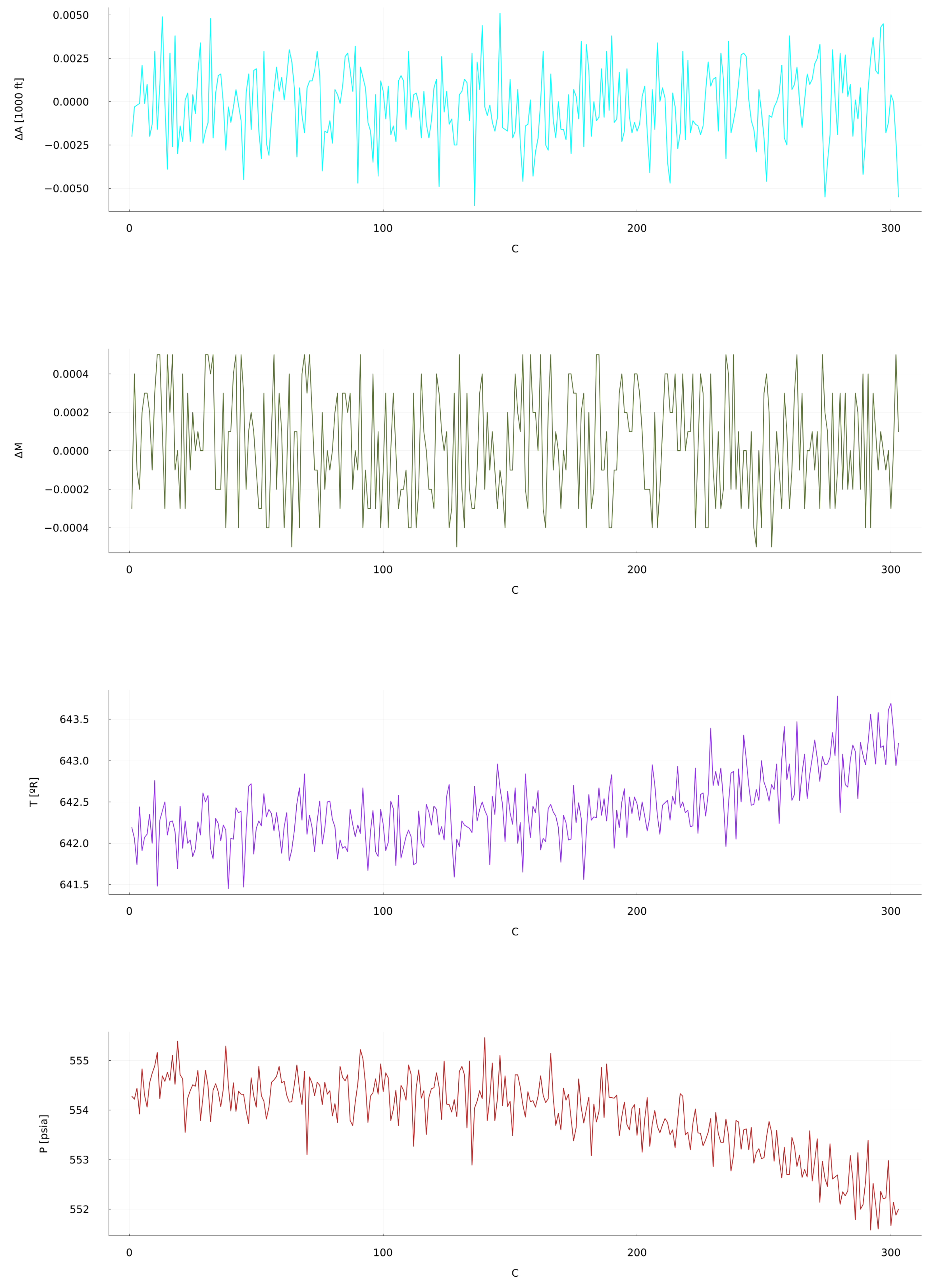
In the CMAPSS dataset the 21 output sensors are directly affected by each other, with the operational settings determining the conditions under which the turbofan engine is working. Predicting how the system is going to react under certain conditions, and specially how each of the components behave, can assist in detecting a specific failure in the engine when certain sensors are off from their nominal values. The time series under study belongs to Unit 49 in the “Test 1” file, focusing on the first two operational settings and two compressor sensors as seen in Figure 2. This has been the selected data for the available length, as it provides enough information for the reservoir to parse through and learn on the behaviour of the turbofan engine.
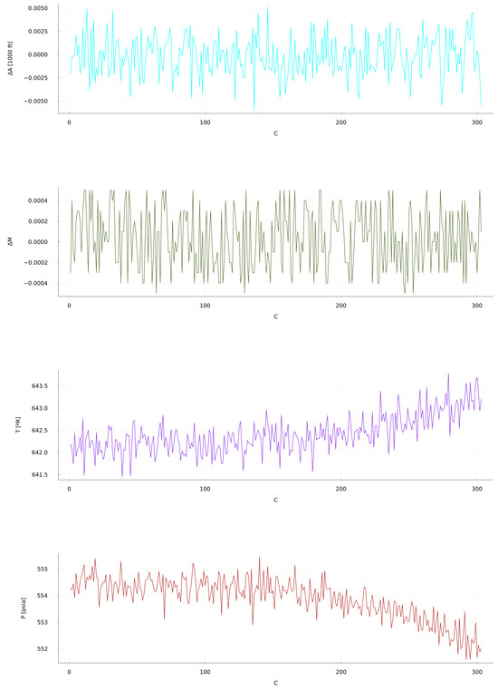
Figure 2.
CMAPSS dataset Test 1, Unit 49 (from top to bottom): OS 1: Altitude, OS 2: Mach Number, Sensor 2: Total temperature at LPC outlet, Sensor 7: Total pressure at HPC outlet. Time units are in operating cycles.
In Table 2 the hyperparameters bounds are shown. These values depend mainly on the size and the complexity of the time series. The selection of these values have followed the standard criteria. In particular, as already said, the size of the reservoir, N, should be high enough to capture the dynamics of the sensor without compromising computational costs. It is usual for N to be at least equal to the estimate of independent real values the reservoir has to remember from the input to solve its task [7]. Thus a reasonable lower estimate is at least nodes. Arbitrarily, we established 10 times that quantity, i.e., , as an upper bound. About the input matrix scaling factor, , it needs to be threefold for this dataset. The first factor is for the unitary value appended to the input, the second is for the OPs and the third is for the output sensors. The establishment of bounds followed, [19] allowing the scaling factors to vary wildly between them so the inputs that are more relevant to the reservoir dynamics are present the most. The rest of the bounds have been established arbitrarily.
Table 2.
Upper and lower bounds for the hyperparameter optimization of the CMAPSS dataset.
3. Results
The CMAPSS dataset grants the option to analyse and minimize the impact of having a limited amount of data, only about three hundred discrete values for each signal. The system has been run for 300 iterations with a population of 50 at each one. The 24 predicted signals (OPs + sensors) differ from the originals, as the reduced amount of training data affects the capacity of the reservoir to track the precise behaviour of the turbofan engine. Nevertheless, some signals are better predicted than others, providing insights into the turbofan engine.
Several runs have been set up for the dataset, to minimize the effect of chance on finding the optimum configuration. From these runs five main sets are of particular notice (shown in Table 3), as most results gravitate towards the viccinity of their hyperparameter sets. The averaged nRMSE over all considered signals is the collective error from the 3 OPs and the 21 sensors, as all are jointly fed to the reservoir and a prediction is generated simultaneously for the 24 time series.
Table 3.
RC-GWO Ensemble optimized hyperparameter sets for the CMAPSS dataset. The nRMSE is averaged over the 24 signals.
Sets 1 and 2 ( and ) generated the predictions with smaller nRMSE. The stark difference resides in the input scaling factors which is over an order of magnitude higher than in other sets. For , with the smallest reservoir size, the three folded scaling factors have similar values, meaning the activation functions will give the unitary, OPs and sensor inputs approximately the same weight towards the calculation of the internal states. Not only the ’s have the same importance, but actually they take high values forcing the activation functions to behave like binary switches. A similar behaviour has been detected for , which even with a greater size still suffers from too high input scaling factors which is detrimental to its predictive capabilities.
Thus, in spite and show smaller averaged nRMSE their reservoir internal states does not guarantee a better individual prediction as, for both of these sets the reservoir internal states are saturated, i.e., most of the neurons yield extreme values (Figure 3 top), instead of being distributed around 0 (Figure 3 bottom). As a consequence the network looses the advantages of the separability granted by the ESP. Reservoir saturation is an aspect that warrants a discussion of its own as it is a phenomenon that severely impacts performance. Saturation is present when the internal states of the reservoir loose scope of the input signal features, which in turn lead to a reduction of its learning capacity. In order to mitigate the chances of this behaviour it is necessary to increase the amount of neurons in the reservoir and limit the input scaling factors to a lesser order of magnitude.
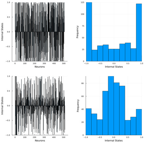
Figure 3.
Internal states of a reservoir. Left: Internal states for each the neuron. Right: histogram for the internal states. Results obtained at an arbitrary step during training. Top: A saturated reservoir. Bottom: an unsaturated reservoir.
Sets , and suggest that reservoir size is not the main hyperparameter acting on the average nRMSE as even though is nearly ten times the size of —and due to the sparsity ten times the computational cost [7]—the error does not reduce proportionately. Due to data shortness increasing the quantity of neurons does not report a decrease in nRMSE, therefore other hyperparameters must be at play to contribute to the prediction error. The leak rate plays the biggest role when generating predictions on limited data. As can be seen on to a higher value may drive the reservoir into forgetting too quickly the original features as the previous internal states are not as influential when updating.
The input scaling factors are similar, or the same order, for –, as the main takeaway is the necessity to attenuate extreme values and augment the actual signals, thus making them the primary drivers of activation. Sparsity does not affect the quality of the predictions as the echo state property can be achieved with fully connected reservoirs. It is known that the only advantage found is the linear increase in computation costs rather than quadratic when increasing the reservoir size.
The spectral radius scaling factor is used to enforce the echo state property through establishing the maximal eigenvalue of the internal weight matrix. Even though it can still be achieved with values greater than 1 it is simpler to keep it bounded below it, taking into consideration that it should be greater in tasks that require longer memory. Therefore the scaling factors of – serve as a support to the leak rate, improving the reservoir capacity to retain the time series features given the limited data. As for the regularization coefficient no clear effect has been found and has only served to ensure stability and prevent overfitting.
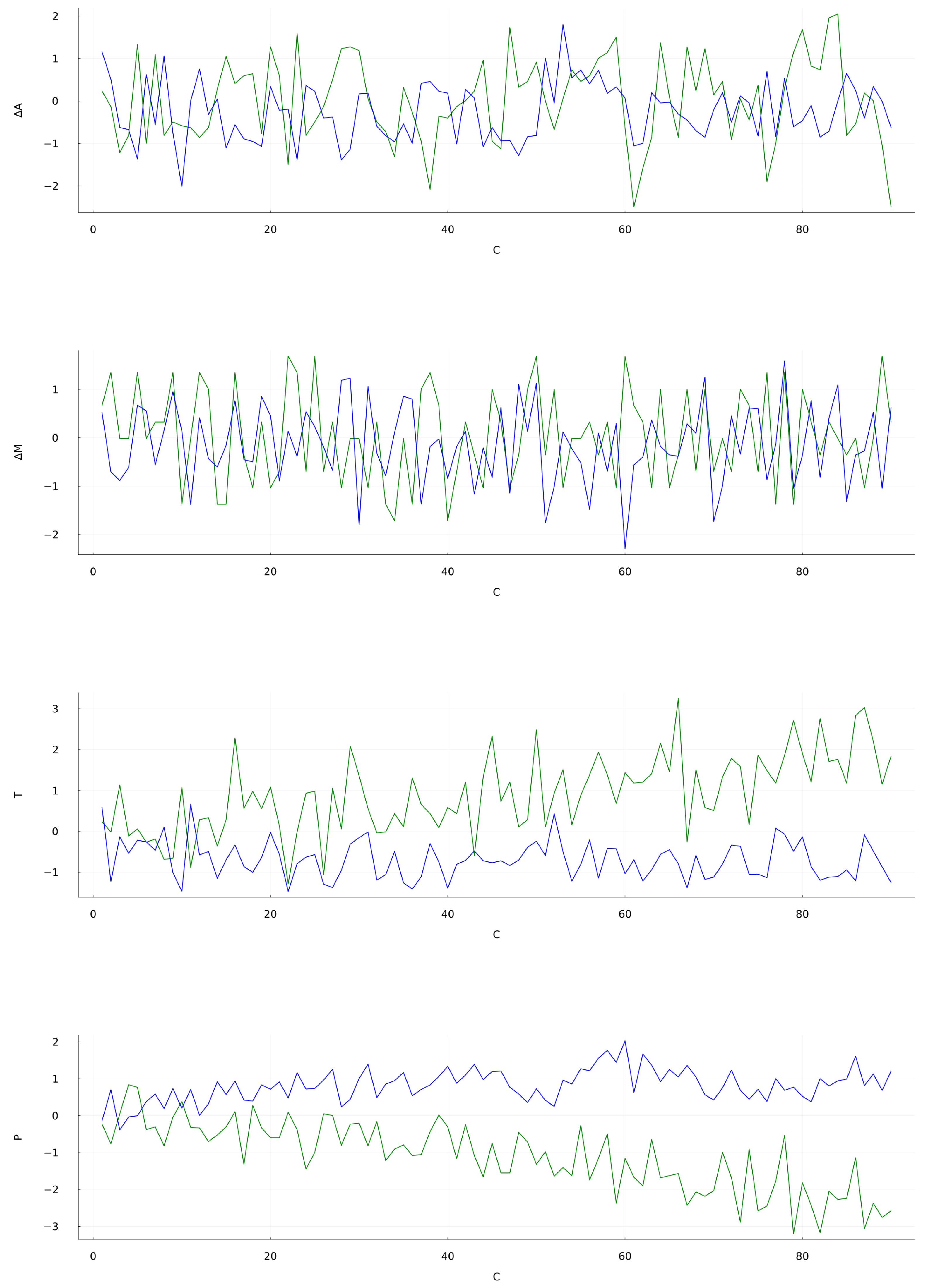
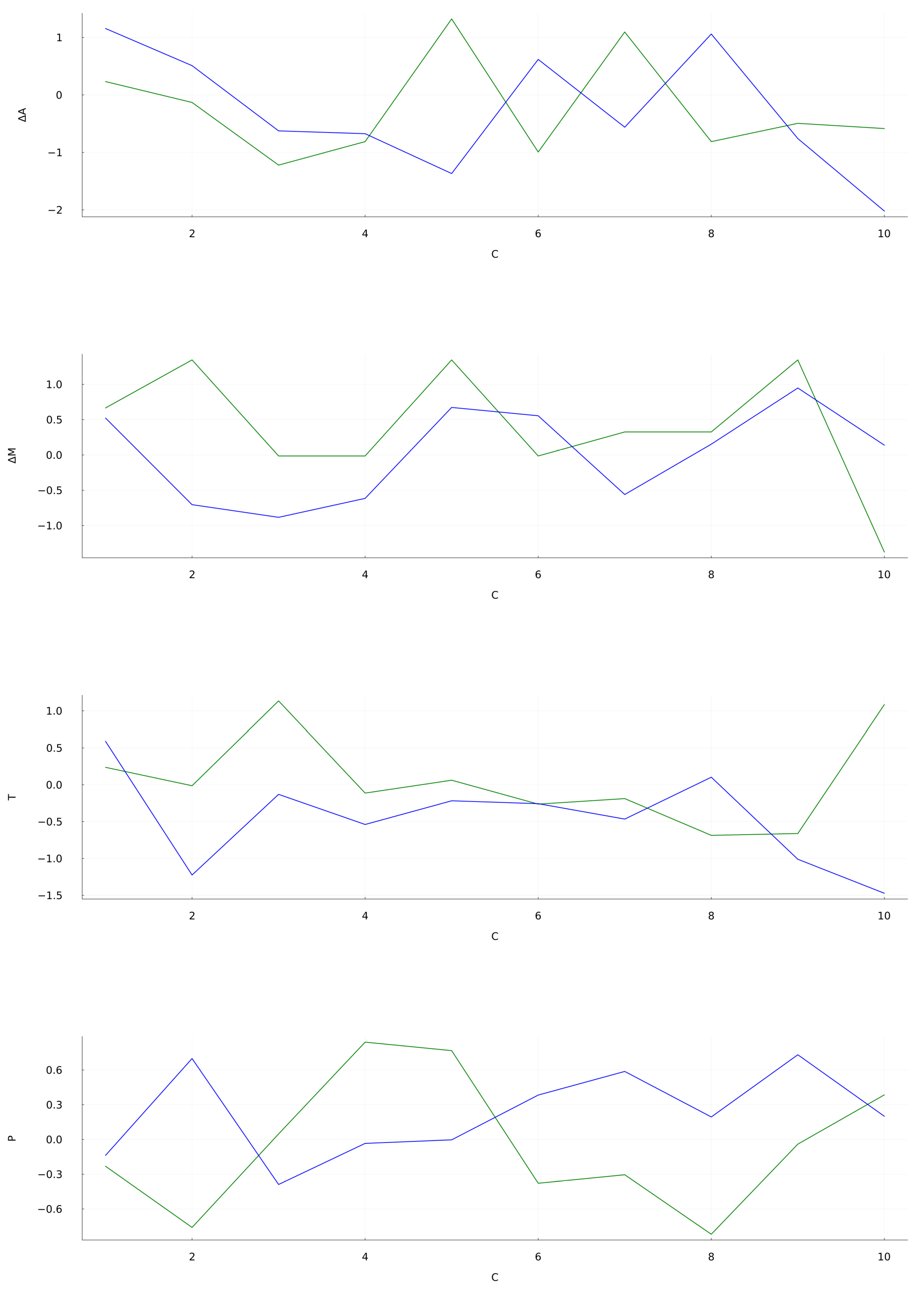
The generated predictions for are shown in Figure 4. It is observed that the overall qualitative behavior of the predicted signal follows the trends of the original signal. In particular, the prediction is bounded between the actual data showing no divergences. The first operational setting at Figure 4 (top) yields an nRMSE of . Even with such an error, the target initial trend are followed closely up to 10 cycles. It is also noticeable the reservoir capacity to follow the drop at 60 cycles. The Mach signal prediction, shown at Figure 4 (bellow top), has an average nRMSE of . This results shows the reservoir capacity to approximately mimic the target data with such a limited training. During the initial 20 cycles the predicted signal closely follows the target, staying within the bounds of the original series. Similar coincidences are observed at the 50 cycles mark and between 60 and 80 cycles. As for the last two signals, Sensor 2 at Figure 4 (above bottom) and Sensor 7 at Figure 4 (bottom), the distance between the prediction and the target grows in an apparently linear fashion as time goes, and as the nRMSE values at Table 4 show. Sensor 2 prediction holds close to the original signal during the first 20 cycles but then undershoots, while Sensor 7 overshoots at the first 10 cycles. Both these predictions miss the mark at replicating the trends of the target. The particular set of hyperparameters for generates an stable and feature-rich prediction that can serve as a baseline for future developments. The behavior of the forecasted signal during the first 10 cycles is shown in Figure 5. In the OS 1, OS 2 and Sensor 2 data the predicted signal approximately follows the target with a small delay. However, sensor 7 data forecast clearly differs from the target. For these four situations the calculated nRMSE are , , and , respectively.
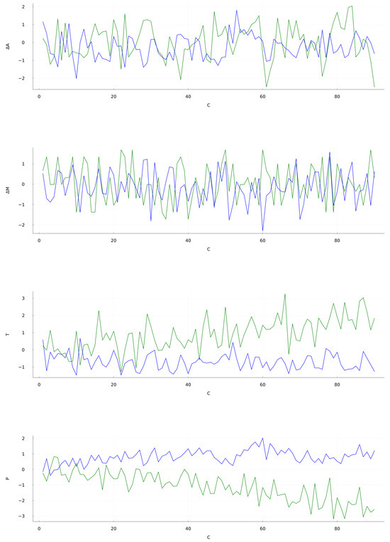
Figure 4.
CMAPSS dataset Test 1, Unit 49 time series prediction for Set 3 (from top to bottom): OS 1: Altitude, OS 2: Mach Number, Sensor 2: Total temperature at LPC outlet and, Sensor 7: total pressure at HPC outlet. Time units are in operating cycles. Green: target signal; Blue: predicted signal. Results for the additional sets are available as Supplementary Materials.
Table 4.
RC-GWO System nRMSE values for the predicted signal values of each of the sets. OS 3 and Signals 1, 5, 10, 16, 17, 18 and 19 remain at a constant value throughout the length of the dataset.
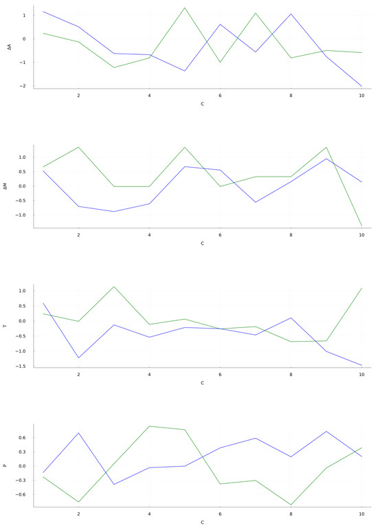
Figure 5.
Zoom detail of the forecasting along the 10 initial cycles. Details are the same as in Figure 4.
4. Conclusions
The optimized hyperparameter sets show promise for generating predictions on a complicated system such as a turbofan engine. Emulating simultaneously the behaviour of 24 signals on a small reservoir can lead to computationally effective and quick results, generating forecasts with the data at hand. The hyperparameters that configure the reservoir need to be finely tuned and understood. Establishing valid bounds for such a task grants the RC-GWO system a greater chance at finding an stable optimum for the time series under study. The sets are capable of generating stable predictions fluctuating at the same range of values of the target. Notoriously, in contrast to works devoted to chaotic dynamical systems that pay attention to the detailed forecasted signal target tracking [20], the few number of works committed to engineering systems usually summarize their finding using the RMSE or similar measures, without reporting tracking results. In our opinion, the actual tracking capabilities of the forecasted signal must be shown not to mask spurious results.
It should be emphasized that the present approach uses the simplest random reservoir. Improvements could allow to detect out of ordinary doings indicating the need for maintenance. Given the complex behavior of the turbofan engine it is expected that a reservoir tuned in a critical state shall improve the predictive capabilities, as criticality has been shown to be optimal for such complex situations [21]. Future works will consider simple networks configurations where criticality is easily achieved [22].
These early stages aim at developing a tool for a comprehensive evaluation of the entire process. It may help to avoid the black-box characteristics of most Machine Learning solutions so the predictions could be understood, evaluated and accepted minimizing the fear of failure that may well pose a safety risk to people, workers and companies. Transparency in the field of Artificial Intelligence is a requirement for the general well-being, assuring users and authorities that these systems are reliable tools rather than cheap shortcuts with special consideration to the specific necessities of the Aerospace industry.
Supplementary Materials
The following material are available online at https://github.com/JMRRiesgo/RC-GWO-System-Data, Figure S1: CMAPSS dataset Test 1, Unit 49 time series prediction for Set 1; Figure S2: CMAPSS dataset Test 1, Unit 49 time series prediction for Set 2; Figure S3: CMAPSS dataset Test 1, Unit 49 time series prediction for Set 4; Figure S4: CMAPSS dataset Test 1, Unit 49 time series prediction for Set 5.
Author Contributions
Conceptualization, J.L.C.F. and J.M.R.R.; methodology, J.L.C.F.; software, J.M.R.R. and J.L.C.F.; validation, J.L.C.F.; formal analysis, J.M.R.R. and J.L.C.F.; investigation, J.M.R.R.; resources, J.M.R.R.; data curation, J.M.R.R.; writing—original draft preparation, review and editing, J.M.R.R. and J.L.C.F.; visualization, J.M.R.R.; supervision, J.L.C.F. All authors have read and agreed to the published version of the manuscript.
Funding
This research received no external funding.
Data Availability Statement
The data supporting reported results can be found at the author’s GitHub repository at https://github.com/JMRRiesgo/RC-GWO-System-Data, accessed on 1 May 2024. The original dataset analyzed during the study can be found at the “Prognostics Center of Excellence Data Set Repository” (NASA) at https://www.nasa.gov/intelligent-systems-division/discovery-and-systems-health/pcoe/pcoe-data-set-repository/, accessed on 15 March 2023.
Acknowledgments
The authors would like to thank the NASA Ames Prognostics Center of Excellence, and in particular to A. Saxena and K. Goebel for making available the data used in this study. This study was carried out as part of a JMRR Master thesis.
Conflicts of Interest
The authors declare no conflict of interest.
Abbreviations
The following abbreviations are used in this manuscript:
| ESP | Echo State Property |
| ESN | Echo State Network |
| GWO | Grey Wolf Optimizer |
| LNN | Liquid Neural Nets |
| LSM | Liquid State Machines |
| nRMSE | normalized Root Mean Square Error |
| RC | Reservoir Computing |
| RNN | Recurrent Neural Network |
References
- Zio, E. Prognostics and Health Management (PHM): Where are we and where do we (need to) go in theory and practice. Reliab. Eng. Syst. Saf. 2022, 218, 108–119. [Google Scholar] [CrossRef]
- Brunton, S. Data-Driven Aerospace Engineering: Reframing the Industry with Machine Learning. AIAA J. 2021, 59, 2820–2847. [Google Scholar] [CrossRef]
- Carvalho, T. A systematic literature review of machine learning methods applied to predictive maintenance. Comput. Ind. Eng. 2019, 137, 106024. [Google Scholar] [CrossRef]
- Gao, C. Medium and Long-Term Fault Prediction of Avionics Based on Echo State Network. Mach. Learn. Deep. Learn. Optim. Tech. Heterog. Sens. Inf. Integr. 2023, 2022, 5343909. [Google Scholar] [CrossRef]
- Rigamonti, M.; Baraldi, P.; Zio, E.; Roychoudhury, I.; Goebel, K.; Poll, S. Echo State Network for the Remaining Useful Life Prediction of a Turbofan Engine. PHM Soc. Eur. Conf. 2016, 3, 5343909. [Google Scholar] [CrossRef]
- Márquez, M.R.; Gutiérrez, E.D.; Álvarez, J.S.M.; Milton, J.G.; Cabrera, J.L. Machine learning forecasting of extreme fluctuations in a human balancing task. Knowl.-Based Syst. 2023, 280, 111000. [Google Scholar] [CrossRef]
- Lukoševičius, M. A practical guide to applying echo state networks. Lect. Notes Comput. Sci. 2012, 7700, 659–686. [Google Scholar] [CrossRef]
- Konkoli, Z. Reservoir Computing. In Encyclopedia of Complexity and Systems Science; Springer: Berlin/Heidelber, Germany, 2017. [Google Scholar] [CrossRef]
- Jaeger, H. The “echo state” approach to analysing and training recurrent neural networks-with an erratum note. In German National Research Center for Information Technology GMD Technical Report; GMD: Bonn, Germany, 2001; Volume 148, p. 13. [Google Scholar]
- Maas, W.; Natschläger, T.; Markram, H. Real-time computing without stable states: A new framework for neural computation based on perturbations. Neural Comput. 2002, 14, 2531–2560. [Google Scholar] [CrossRef] [PubMed]
- Hasani, R.; Lechner, M.; Amini, A.; Rus, D.; Grosu, R. Liquid Time Constant Networks. arXiv 2020, arXiv:2006.04439. [Google Scholar] [CrossRef]
- Pathak, J.; Hunt, B.; Girvan, M.; Lu, Z.; Ott, E. Model-Free Prediction of Large Spatiotemporally Chaotic Systems from Data: A Reservoir Computing Approach. Phys. Rev. Lett. 2018, 120, 024102. [Google Scholar] [CrossRef]
- Cai, H.; Ao, Z.; Tian, C.; Wu, Z.; Liu, H.; Tchieu, J.; Gu, M.; Mackie, K.; Guo, F. Brain organoid reservoir computing for artificial intelligence. Nat. Electron. 2023, 6, 1032–1039. [Google Scholar] [CrossRef]
- Martinuzzi, F. A Brief Introduction to Reservoir Computing. Available online: https://martinuzzifrancesco.github.io/posts/a-brief-introduction-to-reservoir-computing/#3 (accessed on 1 May 2024).
- Jaeger, H. Echo state network. Scholarpedia 2007, 2, 2330. [Google Scholar] [CrossRef]
- Mirjalili, S.; Mirjalili, S.M.; Lewis, A. Grey Wolf Optimizer. Adv. Eng. Softw. 2014, 69, 46–61. [Google Scholar] [CrossRef]
- Saxena, A.; Goebel, K.; Simon, D.; Eklund, N. Damage propagation modeling for aircraft engine run-to-failure simulation. In Proceedings of the 2008 International Conference on Prognostics and Health Management, Denver, CO, USA, 6–9 October 2008. [Google Scholar] [CrossRef]
- Prognostics Center of Excellence Data Set Repository—NASA. Available online: https://www.nasa.gov/intelligent-systems-division/discovery-and-systems-health/pcoe/pcoe-data-set-repository/ (accessed on 4 March 2024).
- Xu, M.; Baraldi, P.; Al-Dahidi, S.; Zio, E. Fault prognostics by an ensemble of Echo State Networks in presence of event based measurements. Eng. Appl. Artif. Intell. 2020, 87, 103346. [Google Scholar] [CrossRef]
- Lu, Z.; Pathak, J.; Hunt, B.; Girvan, M.; Brockett, R.; Ott, E. Reservoir observers: Model-free inference of unmeasured variables in chaotic systems. Chaos 2017, 27, 041102. [Google Scholar] [CrossRef]
- Mandal, S.; Shrimali, M.D. Achieving criticality for reservoir computing using environment-induced explosive death. Chaos 2021, 31, 031101. [Google Scholar] [CrossRef]
- Cabrera, J.L.; Hoenicka, J.; Macedo, D. A Small Morris-Lecar Neuron Network Gets Close to Critical Only in the Small-World Regimen. J. Complex Syst. 2013, 1, 675818. [Google Scholar] [CrossRef]

Disclaimer/Publisher’s Note: The statements, opinions and data contained in all publications are solely those of the individual author(s) and contributor(s) and not of MDPI and/or the editor(s). MDPI and/or the editor(s) disclaim responsibility for any injury to people or property resulting from any ideas, methods, instructions or products referred to in the content. |
© 2024 by the authors. Licensee MDPI, Basel, Switzerland. This article is an open access article distributed under the terms and conditions of the Creative Commons Attribution (CC BY) license (https://creativecommons.org/licenses/by/4.0/).