Towards Resolving the Ambiguity in Low-Field, All-Optical Magnetic Field Sensing with High NV-Density Diamonds ^†

Abstract

In all-optical magnetic field sensing using nitrogen-vacancy-center-rich diamonds, an ambiguity in the range of 0–8 mT can be observed. We propose a way to resolve this ambiguity using the magnetic-field-dependent fluorescence lifetime. We therefore recorded the frequency response of the fluorescence upon modulation of the excitation intensity in a frequency range of 1–$100\mathrm{MHz}$. The magnetic-field-dependent decay dynamics led to different response characteristics for magnetic fields below and above $3\mathrm{mT}$, allowing us to resolve the ambiguity. We used a physics-based model function to extract fit parameters, which we used for regression, and compared it to an alternative approach purely based on an artificial neural network.

1. All-Optical Magnetic Field Sensing with NV Centers

Negatively charged nitrogen-vacancy (NV) centers in diamonds have attracted considerable attention in the area of magnetic field sensing. Most setups are based on the manipulation of spin states using microwave (MW) excitation, realizing high sensitivities and spatial resolutions. However, they come with certain limitations due to the MW delivery, like the interaction of the MW with the environment and the requirement for a galvanic connection. In contrast, all-optical setups rely on exclusive optical access to the sensing volume, allowing the construction of a fiber-based sensor [1,2,3,4]. Such a sensor features a non-magnetic and non-conductive probe and allows the realization of high insulation resistance. Additionally, setups without MW are less complex and easier to implement in industrial applications. All-optical setups can be based on narrow-band features, realizing high sensitivities but requiring stable bias magnetic fields with accurate alignment [5,6,7]. Our setup, in contrast, uses the fluorescence change caused by spin mixing for magnetic fields up to ∼50 mT [1,8]. This allows the sensing of a high bandwidth of magnetic fields without the need for bias fields, realizing a compact and universally applicable sensor head.

Recently, we published an all-optical setup, making use of the excited state lifetime of optically pumped NV centers [9]. The setup is based on the frequency domain fluorescence lifetime measurement, where the excitation light is modulated in its intensity in a sufficiently high frequency range [10]. With increasing frequency, the low-pass characteristic of the fluorescence lifetime will lead to a reduction in the amplitude and a shift in the phase between excitation and fluorescence signals from $0^{\circ }$ to ${90}^{\circ }$. The excited state lifetime components respond to magnetic fields [11,12], which can be observed in an overall change in the frequency response [9]. These studies revealed a high magnetic contrast of the intensity at low excitation frequencies, as well as a maximum in the magnetic contrast of the phase at an excitation frequency of $13\mathrm{MHz}$. The measurement of the phase at a fixed frequency in particular enables a high immunity to fluctuations in the optical path, compared to the measurement of the fluorescence intensity. Such fluctuations can arise, e.g., due to movement in the optical fiber, and would be misinterpreted as magnetic field changes in an intensity-based setup.

In NV-rich diamonds, we observe a dip in the fluorescence intensity at zero magnetic field [4]. Current research relates this dip to dipolar coupling between neighboring NV centers, leading to mixing of spin states [13,14]. The same feature can also be observed when using the phase as a measurement quantity [9]. This leads to an ambiguity, i.e., a non-injective function, for magnetic fields below ∼8 mT. We plot the fluorescence intensity as a function of magnetic fields in the left panel of Figure 1, qualitatively, showing this behavior.

The measurement of phase or intensity at a fixed excitation frequency can be realized with a lock-in amplifier, yielding a high acquisition speed and possibly simpler implementation compared to using a whole frequency sweep. The complete response of magnitude and phase in a frequency range of 1–$100\mathrm{MHz}$, on the other hand, holds more information. In this work, we utilize this to resolve the ambiguity in all-optical magnetic field sensing. First, we prove this ability by fitting the data with a model function and using the fitted parameters for regression. Afterwards, we explore the use of neural networks with the raw spectra as inputs, omitting the fitting process, which is less computationally expensive. These two approaches are shown schematically in Figure 1.

In principle, the use of a bias field greater than $3\mathrm{mT}$ is also possible to overcome this ambiguity problem. However, we would lose the isotropic sensing ability, which is an important feature for implementation in a measurement application [8]. Additionally, a bias field, created, e.g., by a permanent magnet in the fibre head, would lose the properties of a non-magnetic and non-conductive sensor head. This would restrict the universal applicability of the sensor head.

A potential application lies in current sensing in medium- and high-voltage power distribution grids. The fiber-based sensor can realize high insulation resistances and the isotropic sensing ability simplifies its implementation. With the ever-increasing need for transparent power grids [15], the measurement of currents in the grid for the reliable prediction and management of loads is an important factor. This sensing technology may become a simpler and more cost effective alternative to commonly employed current sensors.

2. Materials and Methods

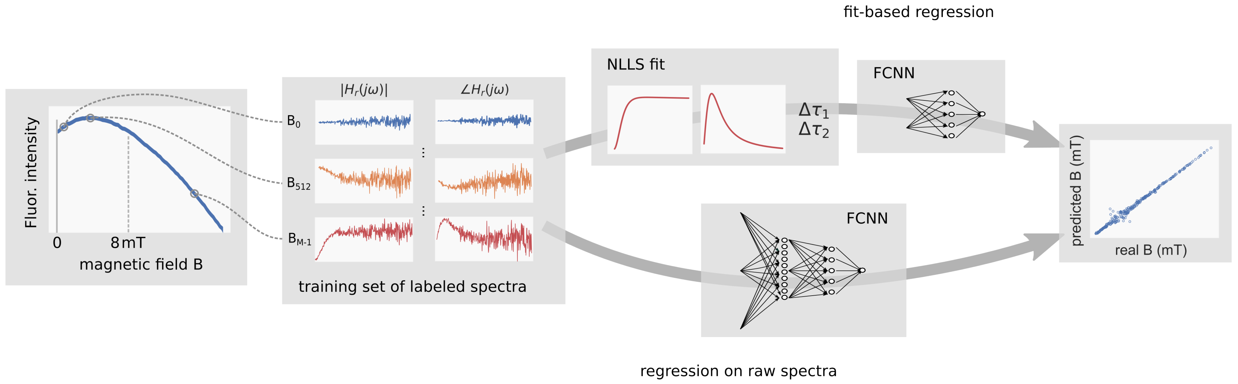
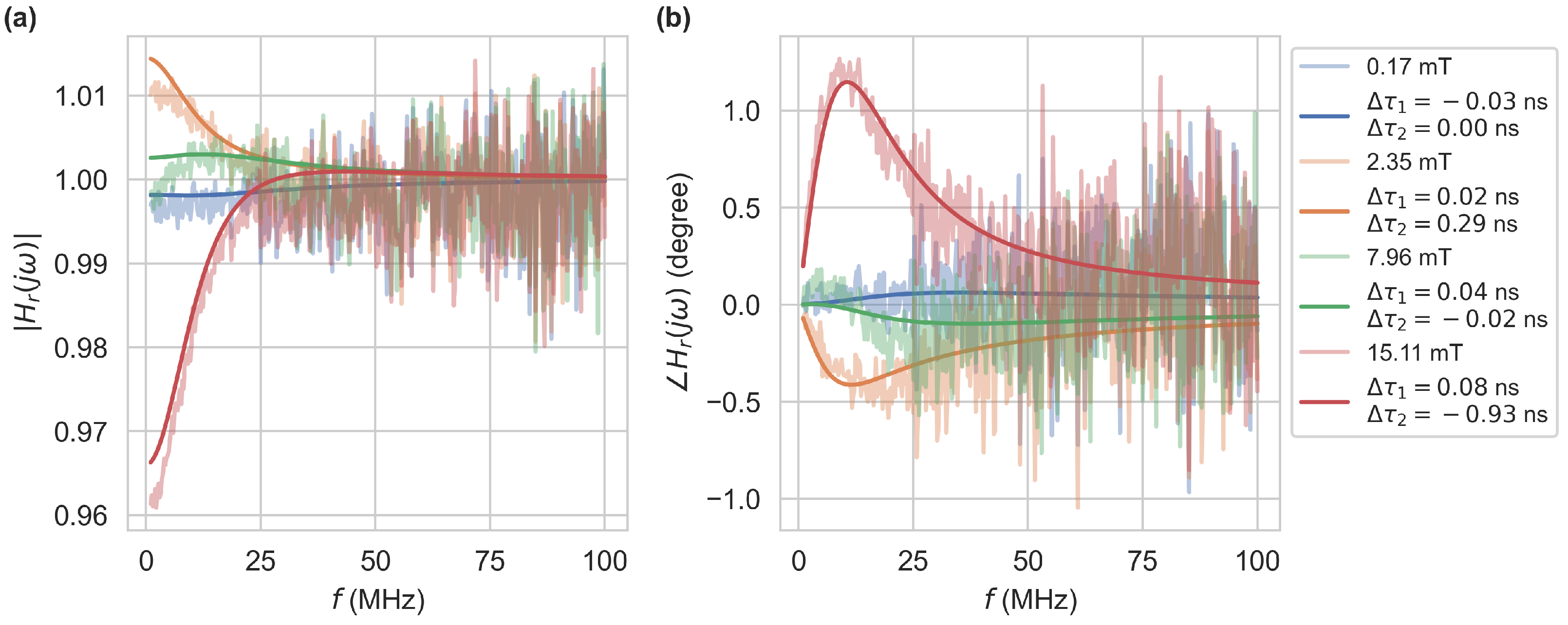
2.1. Frequency Domain Measurement Setup

In Figure 2a, we show the optical and electrical setup used for frequency domain measurements. A collimated $520\mathrm{nm}$ laser diode (ams-OSRAM PLT5 520B) is driven by a laser switch (iC-Haus GmbH iC-HKB) at a mean optical output power of $12\mathrm{mW}$. The input stage of the laser driver is based on a comparator, responsible for switching the laser on or off during positive and negative half waves of the incoming signal. The excitation light is passed through a dichroic mirror (DCM, Thorlabs DMPS567R) and coupled to a $105\mathsf{\mu }\mathrm{m}$ core diameter fibre. The end facet of the fibre is covered in high-NV-density micro-diamonds in glue. The fluorescence of the NV diamonds is collected via the same fiber and passed through a long-pass filter and focused (Thorlabs FELH600 & LA1951-AB) on a photodiode. The photocurrent is amplified and passed to the Vector Network Analyzer (VNA). The VNA sweeps the frequency of the output signal at port one, connected to the laser driver, in a range of 1–$100\mathrm{MHz}$ and records the response in magnitude and phase at port two. An electromagnet, monitored by a Hall effect sensor, is used to apply magnetic fields up to $120\mathrm{mT}$.

2.2. Fit-Based Regression

We operated the system at optical excitation powers for which we expected no saturation behavior [16,17]. In this linear regime, the fluorescence can be interpreted as a convolution of the excitation signal with the decay dynamics. According to a bi-exponential fluorescence decay, the respective transfer function can be written as the sum of two first-order low-pass filters

$$H\left(s\right)=\frac{a_1}{s+\frac{1}{{\tau }_1}}+\frac{a_2}{s+\frac{1}{{\tau }_2}}$$

(1)

with $s=\sigma +j\omega$, following the Laplace-transform of the sum of two exponential functions. The VNA corrects for the system response ${H\left(s\right)|}_{B=0}$ at $B=0$, which we show in Figure 2b. This system response results from all electrical and optical components, necessary for the measurement, as well as the low-pass characteristic of the fluorescence itself. The resulting measurement can be described by the ratio $H_r\left(s\right)=H\left(s\right){{|}_B/H\left(s\right)|}_{B=0}$.

We fitted the recordings of the system response at different B-fields with $H_r\left(s\right)$, using non-linear least squares fitting (NLLS). Therefore we wrote the independent components as their values at $B=0$ and additional B-field dependent terms $\Delta a_1$, $\Delta a_2$, $\Delta {\tau }_1$, and $\Delta {\tau }_2$. To increase the quality of the fit for the application of magnetic field sensing, the fit parameters $a_1=0.65$ and $a_2=0.35$ were fixed, i.e., $\Delta a_1=\Delta a_2=0$. Additionally, the decay times ${\tau }_{1,B=0}$ and ${\tau }_{2,B=0}$ (at zero field) were constrained to be the same for all data sets. The fitting process was carried out in two steps. First, we recorded a set of 30 measurements at different magnetic fields up to $80\mathrm{mT}$ to fit ${\tau }_{1,B=0}$ and ${\tau }_{2,B=0}$. This small set was chosen due to the large necessary computation time. In the second step, we collected 1000 system responses up to $15\mathrm{mT}$ with a distribution favoring low magnetic fields and in a random order. All data sets were fitted individually, with the previously found parameters for ${\tau }_{1,B=0}$ and ${\tau }_{2,B=0}$ set at a constant, yielding $\Delta {\tau }_1\left(B\right)$ and $\Delta {\tau }_2\left(B\right)$. In Figure 3, we show a subset of measured frequency responses at different B-fields with their corresponding fits.

To determine the B field via regression from $\Delta {\tau }_1$ and $\Delta {\tau }_2$ obtained by the fit, we used a small fully connected neural network (FCNN). The network consists of two nodes in the input layer, one hidden layer and an output layer with a single node and linear activation function. The hidden layer is composed of a variable number of neurons, using a ReLU activation function. Using a grid search, we determined an optimum for the number of neurons in the hidden layer, up to a maximum of 60 nodes. We split the observations by ratios of 55%, 15%, and 30% into training, validation and test sets, respectively. During the hyperparameter study, the network’s performance was validated on the validation set. The best network was later trained on the combination of training and validation sets, and the performance was assessed on the test set.

2.3. Regression on Raw Spectra

For the practical applications in magnetometry, NLLS fitting may require too many resources. Therefore, we explore neural networks for regression on the raw system response measurements as input and compare their performance to the fit-based method. Additionally, we focus on the use of FCNNs, which in previous studies have shown a good performance in similar problems. We have also shown the ability of such networks to perform inference in edge-machine learning based setups, enabling the integration of the solution in a practical application [18].

Here, we use an FCNN with three hidden layers, using ReLU activation functions, and vary their sizes to find the network with the lowest complexity which still shows an acceptable performance. Observations are labeled by B and consist of the combination of magnitude $|H_r|$ and phase $\angle H_r$ at 401 different frequencies. Consequently, the input layer consists of 802 nodes. For regression, the output layer has a single node with a linear activation function, like before. Again, we split the observations by ratios of 55%, 15%, and 30% into training, validation and test sets, respectively. The observations are scaled per feature to lie within the interval [0,1] by fitting a MinMaxScaler to the training data and applying it to all data. We used TensorFlow for the implementation and training of the networks [19].

3. Results and Discussion

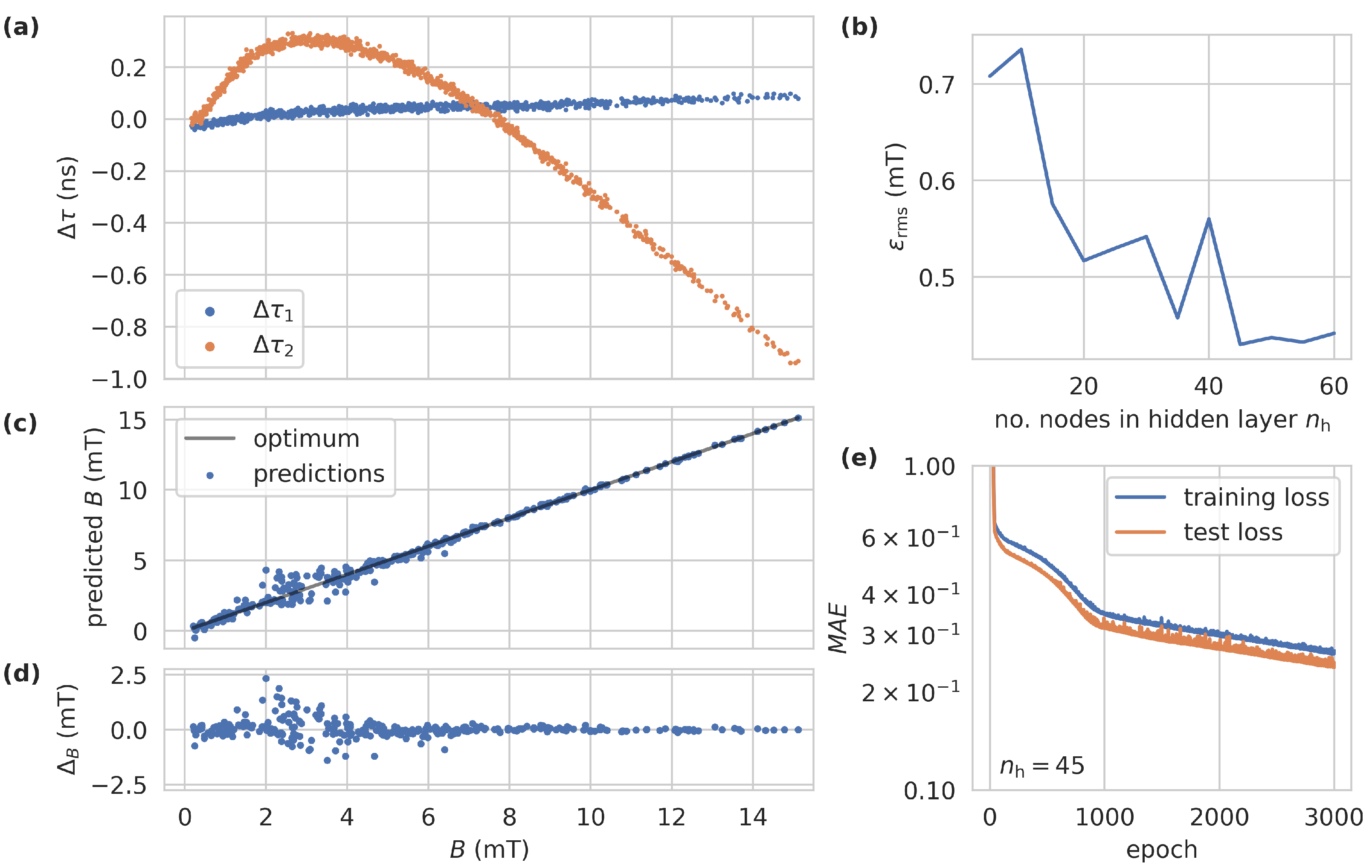
3.1. Fit-Based Regression

In Figure 4a, we show $\Delta {\tau }_1$ and $\Delta {\tau }_2$ as functions of the magnetic field for all data sets. The value $\Delta {\tau }_2$ shows a high responsivity to magnetic fields, but displays the same ambiguity that can be observed in the fluorescence intensity. The monotonically increasing component $\Delta {\tau }_1$, however, aids in resolving this ambiguity. We used these two components as inputs to a simple previously described FCNN to test this hypothesis. In Figure 4b, we show the root-mean-square (RMS) error on the validation set as a function of the number of nodes in the single hidden layer $n_{\mathrm{h}}$. The RMS error declines to a value of around ${ϵ}_{\mathrm{rms}}=0.4\mathrm{mT}$ at 45 nodes and shows no improvement upwards. Therefore, the FCNN was finally trained with $n_{\mathrm{h}}=45$ on the combined training and validation set. We chose the mean average error ($MAE$) as the loss function, shown in Figure 4e on the training and test sets. During the training process, we observed no significant improvement above 800 epochs and the test loss closely followed the training loss, showing no signs of over-fitting. Deeper networks showed no improvements in performance in this task, except for a quicker convergence of the loss function during training.

In Figure 4c,d, we show the predictions of the FCNN as a function of the real magnetic field values on a validation set and the differences from the optimum linear relationship, respectively. Below $2\mathrm{mT}$ and above $4\mathrm{mT}$, the predictions are in good agreement with the real values, within an error of $\pm 0.2\mathrm{mT}$. In the range of 2–$4\mathrm{mT}$, the error rises up to $\pm 2.5\mathrm{mT}$. We attribute this behavior to the low change in both fit parameters ($\Delta {\tau }_1$, $\Delta {\tau }_2$) compared to their variance in this magnetic field range. We observed no outliers, showing that the measurement of magnetic fields below and above ∼3 mT can be distinguished.

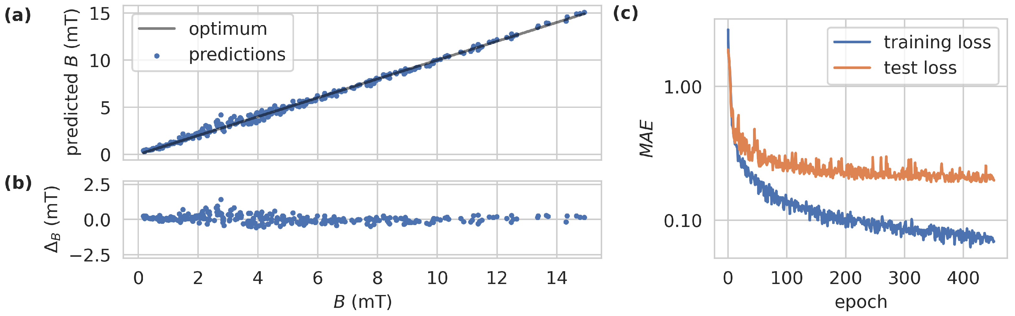
3.2. Regression on Raw Spectra

In a sensing application, the resource requirements for NLLS fitting are likely unpractical. Therefore, we also pursued an alternative approach using a FCNN, where the input consists of the raw system response measurements, i.e., the concatenation of $|H_r|$ and $\angle H_r$. A grid search was carried out to find an optimum for the number of nodes in each of the three hidden layers. The number of nodes varied in the ranges of $n_{\mathrm{h}},1\in [50,200]$, $n_{\mathrm{h}},2\in [20,60]$, and $n_{\mathrm{h}},3\in [5,25]$, where $n_{\mathrm{h},x}$ was the number of nodes in layer x. In Figure 5a,b, we show predictions of the FCNN as a function of the real magnetic field values on a validation set. Therefore, the number of nodes was set to $n_{\mathrm{h},1}=75$, $n_{\mathrm{h},2}=50$, or $n_{\mathrm{h},3}=20$ where the loss showed a minimum. The network was again able to resolve the ambiguity. It performed slightly better than the fit-based approach, with maximum deviations from the real magnetic field of $\pm 1.2\mathrm{mT}$ and an RMS error on the test set of ${ϵ}_{\mathrm{rms}}=0.27\mathrm{mT}$. During training, the $MAE$ on the test set converged quickly and we can see signs of over-fitting from 30 epochs onward (cf. Figure 5c).

On a workstation PC, we found an about 170 times faster execution of this approach, compared to the fit-based regression. This does not account for the previous training, which can be performed in advance in an application.

4. Conclusions

The overall precision of the presented approaches is lower than in all-optical methods based on the measurement of fluorescence magnitude or phase at a single excitation frequency. This holds true especially in the measurement range of 2–$4\mathrm{mT}$. However, we were able to resolve the ambiguity in these setups for magnetic fields below $8\mathrm{mT}$. A setup combining both approaches would be possible, where the electronics switch between VNA and lock-in amplifier mode, depending on the applied magnetic field. Through this, existing setups could benefit from the presented work and construct a sensor system with a high magnetic bandwidth, starting at zero field.

References

1. Fedotov, I.; Amitonova, L.; Sidorov-Biryukov, D.; Safronov, N.; Blakley, S.; Levchenko, A.; Zibrov, S.; Fedotov, A.; Kilin, S.; Scully, M.; et al. Fiber-optic magnetic-field imaging. Opt. Lett. 2014, 39, 6954–6957. [Google Scholar] [CrossRef] [PubMed]
2. Duan, D.; Du, G.X.; Kavatamane, V.K.; Arumugam, S.; Tzeng, Y.K.; Chang, H.C.; Balasubramanian, G. Efficient nitrogen-vacancy centers’ fluorescence excitation and collection from micrometer-sized diamond by a tapered optical fiber in endoscope-type configuration. Opt. Express 2019, 27, 6734. [Google Scholar] [CrossRef] [PubMed]
3. Chatzidrosos, G.; Rebeirro, J.S.; Zheng, H.; Omar, M.; Brenneis, A.; Stürner, F.M.; Fuchs, T.; Buck, T.; Rölver, R.; Schneemann, T.; et al. Fiberized Diamond-Based Vector Magnetometers. Front. Photonics 2021, 2, 732748. [Google Scholar] [CrossRef]
4. Wunderlich, R.; Staacke, R.; Knolle, W.; Abel, B.; Meijer, J. Magnetic field and angle-dependent photoluminescence of a fiber-coupled nitrogen vacancy rich diamond. J. Appl. Phys. 2021, 130, 124901. [Google Scholar] [CrossRef]
5. Wickenbrock, A.; Zheng, H.; Bougas, L.; Leefer, N.; Afach, S.; Jarmola, A.; Acosta, V.M.; Budker, D. Microwave-free magnetometry with nitrogen-vacancy centers in diamond. Appl. Phys. Lett. 2016, 109, 053505. [Google Scholar] [CrossRef]
6. Zheng, H.; Chatzidrosos, G.; Wickenbrock, A.; Bougas, L.; Lazda, R.; Berzins, A.; Gahbauer, F.H.; Auzinsh, M.; Ferber, R.; Budker, D. Level anti-crossing magnetometry with color centers in diamond. arXiv 2017, arXiv:701.06838. [Google Scholar] [CrossRef]
7. Zheng, H.; Sun, Z.; Chatzidrosos, G.; Zhang, C.; Nakamura, K.; Sumiya, H.; Ohshima, T.; Isoya, J.; Wrachtrup, J.; Wickenbrock, A.; et al. Microwave-Free Vector Magnetometry with Nitrogen-Vacancy Centers along a Single Axis in Diamond. Phys. Rev. Appl. 2020, 13, 044023. [Google Scholar] [CrossRef]
8. Staacke, R.; John, R.; Wunderlich, R.; Horsthemke, L.; Knolle, W.; Laube, C.; Glösekötter, P.; Burchard, B.; Abel, B.; Meijer, J. Isotropic Scalar Quantum Sensing of Magnetic Fields for Industrial Application. Adv. Quantum Technol. 2020, 3, 2000037. [Google Scholar] [CrossRef]
9. Horsthemke, L.; Pogorzelski, J.; Stiegekötter, D.; Hoffmann, F.; Langguth, L.; Staacke, R.; Laube, C.; Knolle, W.; Gregor, M.; Glösekötter, P. Excited-State Lifetime of NV Centers for All-Optical Magnetic Field Sensing. Sensors 2024, 24, 2093. [Google Scholar] [CrossRef] [PubMed]
10. Lakowicz, J.R. Principles of Fluorescence Spectroscopy, 3rd ed.; corrected at 4. printing ed.; Springer: New York, NY, USA, 2010. [Google Scholar]
11. Lai, N.D.; Zheng, D.; Jelezko, F.; Treussart, F.; Roch, J.F. Influence of a static magnetic field on the photoluminescence of an ensemble of nitrogen-vacancy color centers in a diamond single-crystal. Appl. Phys. Lett. 2009, 95, 133101. [Google Scholar] [CrossRef]
12. Tetienne, J.P.; Rondin, L.; Spinicelli, P.; Chipaux, M.; Debuisschert, T.; Roch, J.F.; Jacques, V. Magnetic-field-dependent photodynamics of single NV defects in diamond: An application to qualitative all-optical magnetic imaging. New J. Phys. 2012, 14, 103033. [Google Scholar] [CrossRef]
13. Anishchik, S.V.; Vins, V.G.; Yelisseyev, A.P.; Lukzen, N.N.; Lavrik, N.L.; Bagryansky, V.A. Low-field feature in the magnetic spectra of N-V centers in diamond. New J. Phys. 2015, 17, 023040. [Google Scholar] [CrossRef]
14. Akhmedzhanov, R.; Gushchin, L.; Nizov, N.; Nizov, V.; Sobgayda, D.; Zelensky, I.; Hemmer, P. Microwave-free magnetometry based on cross-relaxation resonances in diamond nitrogen-vacancy centers. Phys. Rev. A 2017, 96, 013806. [Google Scholar] [CrossRef]
15. Sun, H.; Huang, S.; Peng, L. High-Current Sensing Technology for Transparent Power Grids: A Review. IEEE Open J. Ind. Electron. Soc. 2024, 5, 326–358. [Google Scholar] [CrossRef]
16. Wee, T.L.; Tzeng, Y.K.; Han, C.C.; Chang, H.C.; Fann, W.; Hsu, J.H.; Chen, K.M.; Yu, Y.C. Two-photon Excited Fluorescence of Nitrogen-Vacancy Centers in Proton-Irradiated Type Ib Diamond. J. Phys. Chem. A 2007, 111, 9379–9386. [Google Scholar] [CrossRef] [PubMed]
17. Magaletti, S.; Mayer, L.; Roch, J.F.; Debuisschert, T. A quantum radio frequency signal analyzer based on nitrogen vacancy centers in diamond. Commun. Eng. 2022, 1, 19. [Google Scholar] [CrossRef]
18. Homrighausen, J.; Horsthemke, L.; Pogorzelski, J.; Trinschek, S.; Glösekötter, P.; Gregor, M. Edge-Machine-Learning-Assisted Robust Magnetometer Based on Randomly Oriented NV-Ensembles in Diamond. Sensors 2023, 23, 1119. [Google Scholar] [CrossRef] [PubMed]
19. Abadi, M.; Agarwal, A.; Barham, P.; Brevdo, E.; Chen, Z.; Citro, C.; Corrado, G.S.; Davis, A.; Dean, J.; Devin, M.; et al. TensorFlow: Large-Scale Machine Learning on Heterogeneous Systems. arXiv 2015, arXiv:1603.04467. [Google Scholar] [CrossRef]
Figure 1. Schematic of the machine learning approach. A data set of labeled spectra at different magnetic fields up to 15 mT is captured and processed in two ways. The spectra consist of the magnitude and phase of the fluorescence from a frequency sweep of the optical excitation up to 100 MHz . They are processed by either fitting a model function with two degrees of freedom and a subsequent simple regression neural network or with a more complex neural network which is trained on the raw spectra.
Engproc 68 00008 g001
Figure 2. (a) Schematic of the optical and electrical setup used for frequency domain measurements. (b) Response of the system at port 2 of the VNA to a frequency sweep at port 1 at B = 0 .
Engproc 68 00008 g002
Figure 3. Subset of measured frequency responses with magnitude | H r | (a) and phase H r (b) at different B-fields and corresponding fits of H r with constant τ 1 , B = 0 = 6.04 ns and τ 2 , B = 0 = 11.89 ns .
Engproc 68 00008 g003
Figure 4. (a) Magnetic-field-dependent changes in lifetimes from fits to frequency responses at τ 1 , B = 0 = 6.04 ns and τ 2 , B = 0 = 11.89 ns . (b) Root-mean-square error of predictions of the simple FCNN on the validation set as a function of the number of hidden nodes n h . (c) Overlay of predictions of the FCNN ( n h = 45 ) on the test set in comparison to the optimum linear relationship. (d) Differences in predictions in (c) to the linear function. (e) Mean average error in the training and test set during the training of the FCNN.
Engproc 68 00008 g004
Figure 5. (a) Overlay of predictions of the FCNN ( n h , 1 = 75 , n h , 2 = 50 , n h , 3 = 20 ) on the test set in comparison to the optimum linear relationship. (b) Differences in predictions in (a) compared to the linear function. (c) Mean average error in the training and test set during the training of the FCNN.
Engproc 68 00008 g005
Disclaimer/Publisher’s Note: The statements, opinions and data contained in all publications are solely those of the individual author(s) and contributor(s) and not of MDPI and/or the editor(s). MDPI and/or the editor(s) disclaim responsibility for any injury to people or property resulting from any ideas, methods, instructions or products referred to in the content.