Abstract
Contamination poses a significant risk to public health by degrading water quality in water distribution systems (WDSs). As one of the key tasks of a response strategy to contamination incidents in a WDS, pipe system flushing has been widely implemented in practice. However, due to the complexity of the network structure and chemical reaction within the pipe system, determining the flushing duration is still one of the significant challenges for a given network. To address this problem, a model for determining the flushing duration is developed. This model is based on calculating the traveling trajectory of the contaminant inside the network. This is carried out by discretizing the one-dimension advection equation and calculating the variation of the contaminant concentration from one segment to another over time. As a preliminary study, we focus on simplified scenarios where contaminants exhibit no chemical reaction within the WDS. The proposed model is applied and analyzed through a simulation study and a laboratory testbed. The results demonstrate the efficacy of the model for determining flushing duration, which can offer valuable insights for real-world applications and serve as a crucial reference for water utility companies.
1. Introduction
Nowadays, water distribution systems (WDSs) face diverse threats to water quality, whether intentional or unintentional, stemming from potential releases of various contaminants. Responding to contamination is pivotal, with pipe flushing emerging as one of the most impactful management strategies for restoring water quality in WDSs. This method involves utilizing hydrant flows or increasing demand at terminal nodes and is widely embraced within the industry [1,2,3]. Understanding specific details of flushing processes, such as flushing time, is crucial for water utility. However, a comprehensive study in this area is lacking from both analytical and practical perspectives.
This paper introduces a model to determine flushing time, which is implemented and validated with simulation results in comparison to EPANET [4]. In addition, experimental results from a testbed verify the validity of the proposed model.
2. Materials and Methods
In this study, contamination without chemical reaction during transportation and flushing is considered. Therefore, the one-dimensional advection equation that neglects dispersion is expressed as follows [2]:
where concentration (mass/volume) in a pipe as a function of distance and time , and flow velocity (length/time) in the pipe. The initial value of this equation is representing the water quality in the pipe at the beginning of the flushing. We assume that the pipe is contaminated with the concentration of the contaminant and is to be flushed by clean water with concentration as shown in Figure 1.
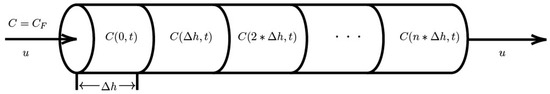
Figure 1.
Space discretization of the pipe to be flushed.
We discretize Equation (1) in space through a backward finite difference:
where is a finite step size, which is the pipe length of each element we divide, as shown in Figure 1. In this way, the pipe is separated into a number of elements with the same volume. In addition, we assume that the flushing water will be mixing completely with the contaminated water in each element. At , which is the first element in the pipe, we have:
where is a time constant. At , we have:
Similarly, a general description can be formulated as:
Equation (5) presents a polynomial function describing the contamination concentration within the n-th element of the pipe during the flushing process. We can solve this equation to calculate the distribution of the contaminant concentration across the entire pipe throughout the flushing duration, i.e., the flushing process will be ended, when the contaminant concentration is lower than a given threshold.
3. Results
Figure 2a shows the simulation results obtained from EPANET for a given pipe. Figure 2b illustrates the solution of Equation (5) using MATLAB [5]. The benchmark scenario involves a pipe with a length of 150 cm and a diameter of 2 cm. Initially, the contaminant concentration within the pipe is 5.6 g/L. Subsequently, flushing water with a concentration of 0.6 g/L and a velocity of 8.49 cm/s is introduced to improve the water quality in the pipe. The duration of water flow through the pipe is approximately 17.6 s.
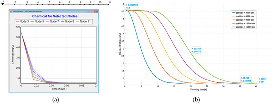
Figure 2.
(a) Flushing process from EPANET; (b) flushing process with our model.
The results obtained from both the EPANET simulation and our model exhibit remarkable similarity. Figure 2b provides further insights into the flushing dynamics. The complete flushing process lasts about 40 s. Notably, at around 35.2 s, which corresponds to twice the flow-through time, the water quality within the pipe closely reaches that of the flushing water.
Figure 3 depicts the flushing process observed in an experimental pipe within a testbed at our laboratory. For the test, we used a flow rate sensor in the pipe and a conductivity sensor at the end of the pipe. A controllable valve was used at the end of the pipe, working as a hydrant during flushing. Figure 3 consists of the conductivity of the water (upper panel), the flow rate within the pipe (middle panel), and the openness of the hydrant valve. It can be seen that, initially, the pipe was contaminated with water possessing a conductivity of 5.6 mS/cm. Flushing commenced following the opening of the hydrant and the start of the flow within the pipe. The flushing process commenced at the 28th second. According to the result illustrated in Figure 2b, the flushing process concluded at the 68th second, with the conductivity reaching approximately 0.76 mS/cm.
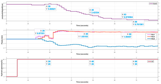
Figure 3.
The flushing process in a testbed.
To further analyze the flushing process, we compared the water quality at two specific time points: halfway through the flushing process (i.e., at the 20th and 48th seconds). At these time points, the concentration and conductivity were observed to be 47.14% and 43.21%, respectively, compared to the initial values. At the twice the flow-through time, the corresponding values were reduced to 12.14% and 17.32%, respectively. This validates our calculated result using the proposed model.
4. Conclusions
This paper introduces a model for estimating the flushing time of contamination in a pipe. The validity of this model is demonstrated through the results obtained from EPANET, MATLAB, and experiments conducted on a testbed. In addition, we identified that twice the flow-through time serves as a critical reference point, indicating when the contaminant concentration within the pipe reaches close to that of the flushing water. This result has a significant implication for water utility companies to deal with contamination incidents. Integration of this model into an optimization framework can be a further step to enhance the efficiency of flushing strategies in WDSs.
Author Contributions
Conceptualization, H.C. and P.L.; methodology, H.C. and P.L.; software, H.C.; validation, H.C.; formal analysis, P.L.; investigation, H.C.; resources, P.L.; data curation, P.L.; writing—original draft preparation, H.C.; writing—review and editing, P.L.; visualization, H.C.; supervision, P.L.; project administration, P.L.; funding acquisition, H.C. All authors have read and agreed to the published version of the manuscript.
Funding
This research is partially supported by the BMBF project MoDiCon with project number of 02WIL1553A.
Institutional Review Board Statement
Not applicable.
Informed Consent Statement
Not applicable.
Data Availability Statement
The datasets and simulation results presented in this paper are available upon request from the corresponding author.
Conflicts of Interest
The funders had no role in the design of the study; in the collection, analyses, or interpretation of data; in the writing of the manuscript; or in the decision to publish the results.
References
- Berglund, E.Z.; Pesantez, J.; Rasekh, A.; Shafiee, E.; Sela, L.; Haxton, T. Review of Modeling Methodologies for Managing Water Distribution Security. J. Water Resour. Plan. Manag. 2020, 146, 03120001. [Google Scholar] [CrossRef] [PubMed]
- Alfonso, L.; Jonoski, A.; Solomatine, D. Multiobjective optimization of operational responses for contaminant flushing in water distribution networks. J. Water Resour. Plan. Manag. 2010, 136, 48–58. [Google Scholar] [CrossRef]
- Friedman, M.; Kirmeyer, G.J.; Antoun, E. Developing and implementing a distribution system flushing program. Am. Water Work. Assoc. 2002, 94, 48–56. [Google Scholar] [CrossRef]
- Rossman, L. EPANET 2.0 User Manual; USEPA: Cincinnati, OH, USA, 2000. [Google Scholar]
- Matlab. Starting Matlab; The MathWorks: Natick, MA, USA, 2012. [Google Scholar]


Disclaimer/Publisher’s Note: The statements, opinions and data contained in all publications are solely those of the individual author(s) and contributor(s) and not of MDPI and/or the editor(s). MDPI and/or the editor(s) disclaim responsibility for any injury to people or property resulting from any ideas, methods, instructions or products referred to in the content. |
© 2024 by the authors. Licensee MDPI, Basel, Switzerland. This article is an open access article distributed under the terms and conditions of the Creative Commons Attribution (CC BY) license (https://creativecommons.org/licenses/by/4.0/).