Multi-Model Demand Forecasting in Water Distribution Network Districts ^†

Abstract

A multi-model including three modelling elements is developed to solve the Battle of Water Demand Forecasting problem. The first two modelling elements working in parallel are a pattern-based algorithm and a Random Forest model. By varying the algorithm setting and predictors, 42 algorithms are constructed and calibrated using demand and weather data in the previous weeks to the generic n-th week, when the objective is the prediction of the hourly demand pattern in the n + 1-th week. Then, a third modelling element is used, which consists of an optimizer aimed at combining the results yielded by the 42 algorithms by analyzing algorithm performance in the n-th week. The same algorithm combination is used to forecast demand at the n + 1-th week.

1. Introduction

Demand forecasting is useful to water utilities for managerial purposes, including the planning of treatment plants and wells and the regulation of pumps, valves, and other controls to ensure water supply [1].

In the context of short-term demand forecasting, which is the topic of the Battle of Water Demand Forecasting (BWDF), various kinds of algorithms have recently been proposed in the scientific literature, including pattern-based algorithms [2] and artificial intelligence [3], with no clear indication of the best modelling approach to use in each problem [4]. This work presents a multi-model approach to overcome the difficulties in the choice of the most suitable algorithm [5]. The following sections describe the methods and applications, followed by the discussion of the results.

2. Methods

The multi-model developed in the present work includes three modelling elements, operating as is described below for the prediction of the hourly demand pattern in a week for a district metered area (DMA) inside the water distribution network. The first two elements work in parallel to supply an optimizer (third modelling element), which aims to identify the best combination of contributions to maximize the forecast performance.

The first modelling element is a pattern-based model. For each district, an hourly demand pattern is defined at the current week by averaging the 168 hourly demands over the past weeks. The demand at the average of the 168 h of the new week is obtained by summing the pattern demand in that hour and a deviation, calculated as a linear function of the deviations in the current week. The coefficients of this linear function are obtained by the Lasso-regularized regression [6], to limit the number of inputs to the most significant ones. Overall, 40 algorithms were obtained from the pattern-based model by changing the size of the weeks on which the averaging is performed and by including/excluding the meteorological variables.

The second modelling element is a Random Forests model [7], which operates by constructing a multitude of decision trees at the training time for each district. In this model, the dependent variable is considered as the demand value at the generic hour and district, while the independent variables include the month, day of the week, hour, and an indicator lumping the information obtained from available meteorological observations. Two algorithms are derived from Random Forests, one considering and the other neglecting the meteorological indicator, respectively.

Given n and n + 1 as indices representing the current week and the week to be forecasted, the 40 algorithms obtained through the pattern-based model are calibrated by considering the hourly demand data observed during weeks from n − 35 to n − 1 (and the hourly meteorological data observed during weeks from n − 34 to n whether required). Conversely, the two algorithms obtained by means of Random Forests were calibrated using the hourly demand data observed during weeks from n − 20 to n − 1 (and the hourly meteorological data observed during weeks from n − 19 to n whether required). Subsequently, the 42 algorithms were employed to forecast the n-th and n + 1-th weeks.

A bi-objective optimization was then applied to demand patterns predicted in the n-th week (validation week), as demand data at the n-th week are indeed known. The objective is to estimate the optimal linear combination of forecasted demand patterns. The optimization was applied twice, considering a different pair of objective functions. In the first application, the objective functions are the first two fitting metrics proposed by the BWDF organizers for the first 24 h of the prediction, i.e., the mean absolute error and the maximum absolute error. In the second application, the objective functions are the third metric proposed by the BWDF organizers for the following 144 h, i.e., the mean absolute error and its standard deviation from week n − 20 to week n. The rationale for the use of the standard deviation is the potentially large variation in the prediction performance observed for the demand from hour 25 to hour 168, as these demand values are temporally far from the latest data available for the previous week. In each optimization application, the decision variables are 42, each of which ranges from 0 to 1, to express the contribution of the generic algorithm to the overall prediction.

The final solution is selected from the Pareto front obtained in the bi-objective optimization using a regret analysis. This is achieved by applying a criterion based on the minimum value of the sum of dimensionless objective functions (forecasting errors). These objective functions are calculated as the ratio of the objective function values to the respective minimum values found in the front. The two optimal combinations of algorithms obtained for the n-th week are then used for demand forecasts at the n + 1-th week, which were submitted as final solutions to the BWDF organizers. Manual adjustments were made only on holidays inside the week, considering the patterns observed in the same holidays in the previous year.

3. Applications

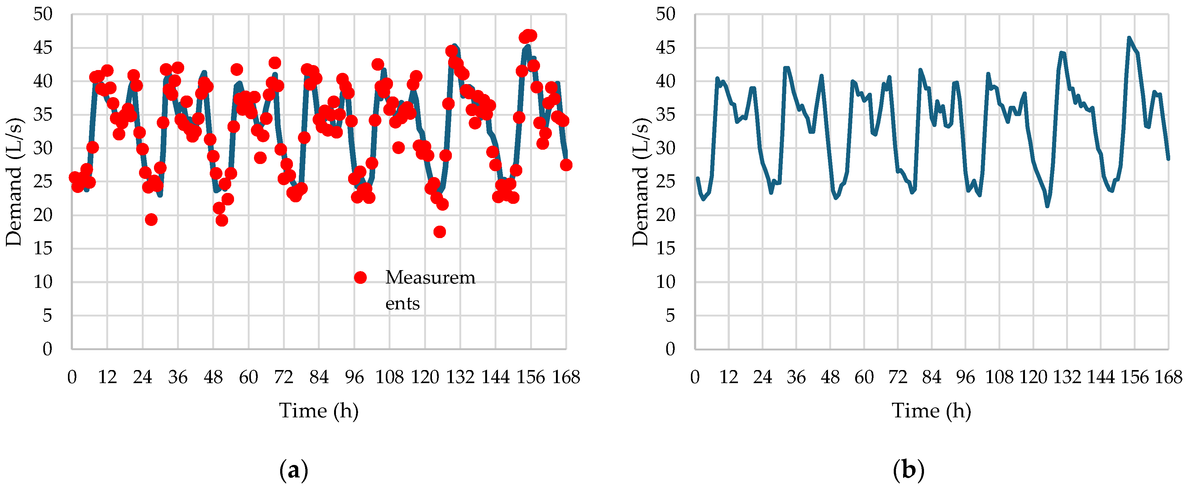
3.1. Case Study

The case study proposed by the BWDF organizers is made up of ten DMAs with various characteristics [1]. As four prediction periods were requested by the BWDF organizers, namely week 25–31 July 2022, week 31 October–6 November 2022, week 16–22 January 2023 and week 6–12 March 2023, the methodology described in Section 2 was applied forty times, i.e., to each of the ten DMAs and to each of the four forecasting periods.

The pattern-based model and the bi-objective optimization were implemented/applied in the Matlab^® 2023b environment. Random Forests was applied in Python 3.7.

3.2. Results

As an example of the results obtained, the output from the third modelling element, i.e., the bi-objective optimization algorithm, is reported below for DMAd and for the last prediction period. Figure 1 depicts the Pareto fronts obtained in the first (Figure 1a) and second (Figure 1b) bi-objective optimizations, along with the selected ultimate solutions concerning contribution coefficients of the 42 demand-forecast algorithms for the hours 1–24 and 25–168, respectively. This solution features the following values for the three error metrics proposed by the BWDF organizers: 1.565 L/s, 4.313 L/s, and 1.921 L/s.

The two optimal combinations of algorithms were then used to predict the demand of DMA d at the n-th week for hours 1–24 and 25–168, respectively, yielding the results shown in Figure 2a in comparison with available demand measurements. Then, they were also used to predict the demand of DMA d at the n + 1-th week (see Figure 2b), which was delivered to the BWDF organizers, along with the predictions for the other DMAs and prediction periods.

4. Discussion

The methodology developed for this work features various innovative aspects, such as the following:

• It combines various methodological approaches to bring the good aspects of each approach into the prediction.
• By using the n-th week as the validation period and by optimizing the prediction on this week, it gives an estimation of the first attempt of the error metrics to be expected at the n + 1-th week, which must be delivered to the BWDF organizers.
• By changing modelling settings, many algorithms are produced in the first two methodological steps to feed the optimization.
• The carrying out of the optimization according to the bi-objective approach results in a trade-off between the various error metrics.
• The double application of the bi-objective optimization yields the optimal combination of algorithm contributions separately for the first day and for the following six days of the week to be delivered for each DMA and prediction period.

References

- Battle of Water Demand Forecast Organizers. Battle of Water Demand Forecasting. Available online: https://wdsa-ccwi2024.it/wp-content/uploads/2024/01/BWDF_Instructions_rev4.pdf (accessed on 20 January 2024).
- Alvisi, S.; Franchini, M.; Marinelli, A. A short-term, pattern-based model for water-demand forecasting. J. Hydroinform. 2007, 9, 39–50. [Google Scholar] [CrossRef]
- Lorente-Leyva, L.L.; Pavón-Valencia, J.F.; Montero-Santos, Y.; Herrera-Granda, I.D.; Herrera-Granda, E.P.; Peluffo-Ordóñez, D.H. Artificial Neural Networks for Urban Water Demand Forecasting: A Case Study. J. Phys. Conf. Ser. 2019, 1284, 012004. [Google Scholar] [CrossRef]
- Donkor, E.A.; Mazzucchi, T.A.; Soyer, R.; Robertson, J.A. Urban Water Demand Forecasting: Review of Methods and Models. J. Water Resour. Plan. Manag. 2014, 140, 146–159. [Google Scholar] [CrossRef]
- Herrera, M.; Torgo, L.; Izquierdo, J.; Pérez García, R. Predictive models for forecasting hourly urban water demand. J. Hydrol. 2010, 387, 141–150. [Google Scholar] [CrossRef]
- Tibshirani, R. Regression shrinkage and selection via the lasso. J. R. Stat. Soc. Ser. B 1996, 58, 267–288. [Google Scholar] [CrossRef]
- Ho, T.K. The Random Subspace Method for Constructing Decision Forests. IEEE Trans. Pattern Anal. Mach. Intell. 1998, 20, 832–844. [Google Scholar]
Disclaimer/Publisher’s Note: The statements, opinions and data contained in all publications are solely those of the individual author(s) and contributor(s) and not of MDPI and/or the editor(s). MDPI and/or the editor(s) disclaim responsibility for any injury to people or property resulting from any ideas, methods, instructions or products referred to in the content. |
© 2024 by the authors. Licensee MDPI, Basel, Switzerland. This article is an open access article distributed under the terms and conditions of the Creative Commons Attribution (CC BY) license (https://creativecommons.org/licenses/by/4.0/).
Share and Cite
Creaco, E.; Giudicianni, C.; Herrera, M. Multi-Model Demand Forecasting in Water Distribution Network Districts. Eng. Proc. 2024, 69, 188. https://doi.org/10.3390/engproc2024069188
Creaco E, Giudicianni C, Herrera M. Multi-Model Demand Forecasting in Water Distribution Network Districts. Engineering Proceedings. 2024; 69(1):188. https://doi.org/10.3390/engproc2024069188
Chicago/Turabian StyleCreaco, Enrico, Carlo Giudicianni, and Manuel Herrera. 2024. "Multi-Model Demand Forecasting in Water Distribution Network Districts" Engineering Proceedings 69, no. 1: 188. https://doi.org/10.3390/engproc2024069188
APA StyleCreaco, E., Giudicianni, C., & Herrera, M. (2024). Multi-Model Demand Forecasting in Water Distribution Network Districts. Engineering Proceedings, 69(1), 188. https://doi.org/10.3390/engproc2024069188