Abstract
The manufacturing industry, with globalization and information technology, is facing cost pressure, low profits, technology difficulties and many other challenges. Enterprises need to strengthen cost management, improve production efficiency, and meet customer demand to cope with the increasingly complex competitive market. Here, our research in this area becomes important. This paper presents a new approach for building a smart decision-making process specifically in manufacturing organizations in terms of profitability. It emphasizes the importance of profitability-based decision making. The basic steps and modules required to build a profitability-based decision process are described. The advantages of this decision-making system are that it can help companies maximize profits, increase productivity, and meet customer demand for order adjustments.
1. Introduction
The manufacturing industry is growing rapidly and needs to adjust in time to face the changing market. Facing different problems in decision making, scheduling and production, especially while at the same time facing different orders for products with different production processes, raw material supplies, production cycles, delivery times, net profits and factory capacities not being fixed, in the process of the past production experience or the current state of production, as well as forecasting the future production demand, will generate a large amount of data; we need to analyze that data, with modeling and sequencing, to seek the production optimal solution to balance all mentioned aspects [1]. The pursuit of manufacturing enterprises to maximize profits while improving production efficiency to meet customer demand, helps manufacturing enterprises to adapt to market demand and smooth development. However, the existing, similar literature research mainly focuses on the impact of AI, big data or queuing theory, unilateral or multifaceted, on the manufacturing industry’s decision-making. We seek an effective method to simultaneously ensure that the enterprise maximizes profits and improves production efficiency [2,3,4].
The paper is to present an approach for building a smart decision-making process that adopts model combinations to conduct qualitative research. A specific problem will be described by constructing a combined mathematical model or a theoretical model, and, at the same time, will demonstrate the operational principle and process by demonstrating the solution.
The main objective is to help manufacturing companies to obtain the maximum profit value, avoid unnecessary profit loss due to production sequencing decision-making without an optimal solution, and at the same time to achieve cost reduction and efficiency, streamline redundancy, improve productivity and satisfy the customer’s requirements at any time by arranging the appropriate configuration of production services [5]. This decision-making process solves the problem of order scheduling and production sequencing confusion, and customer modification needs over a period of time. We only need to repeat the cycle of this decision-making process: accounting, stratification and sequencing, and then scheduling and production [6,7,8,9].
2. Concept of Proposed Approach in Terms of Profitability
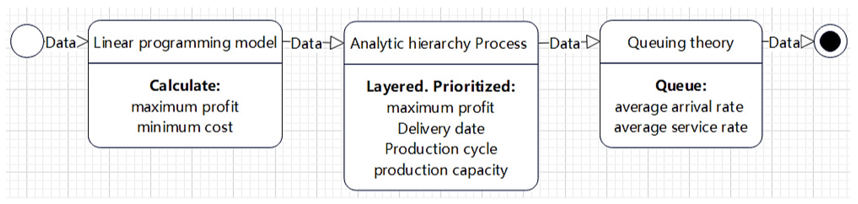
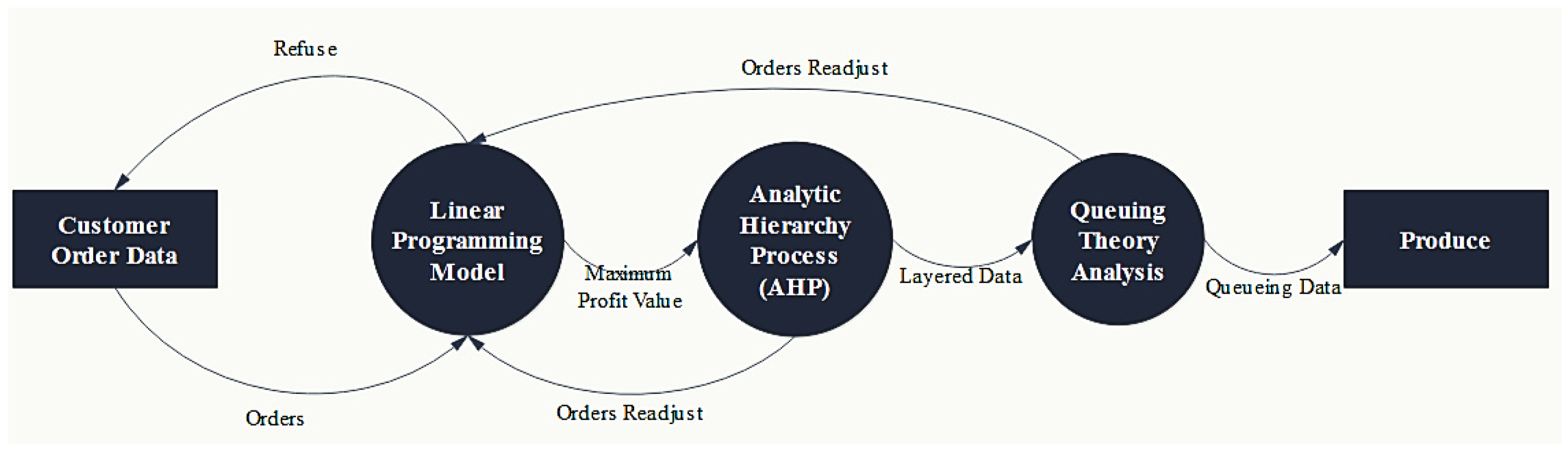
The concept of the approach for building a smart decision-making process in terms of profitability that is based on three steps is described in this section, as Figure 1 illustrates the analytic hierarchy process and the queuing theory model in series.
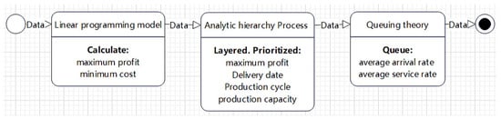
Figure 1.
The analytic hierarchy process and the queuing theory model in series.
In today’s fierce market environment, corporate profits have been compressed. At the same time, due to poor production decisions by manufacturing companies, the company will be unable to achieve maximum profits, forcing the company to face a more severe situation. An efficient and orderly decision-making production method is proposed based on ensuring profitability that is focused mainly on manufacturing companies obtaining maximum benefits under the constraints of limited production conditions (such as: the quantity limit of production equipment) and production materials, while improving production efficiency and meeting customer needs [10]. The process is divided into 3 steps:
Step 1: Use the linear programming model to calculate the maximum profit and select the appropriate production order;
Step 2: Use the four index factors of the Analytical Hierarchy Process to hierarchically arrange the production order of the orders to ensure that the company gives priority to the most suitable orders under limited production conditions and production materials. (Four indicator factors: maximum profit, production cycle, delivery date, production capacity).
Step 3: Use queuing theory to queue up production and improve production efficiency to meet customer needs.
The theoretical derivation analysis and software programming simulation deductions are conducted for this solution to determine its effectiveness and feasibility. In this process, we need to drill the plan, improve and optimize individual indicator values, and achieve optimal results through continuous testing and optimization. Finally, we need to evaluate the proposed solution to determine its actual application effect and make corresponding improvements or adjustments [11,12].
Figure 2 presents the flow and circulation of the entire decision-making process. We will use the series command of the software MATLAB (R2024a) to connect the three models in series, and perform order data analysis, calculation layering and queuing. The following are the model series instructions and process:
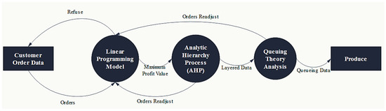
Figure 2.
The whole work flow chart.
Grammar:
- series
- sys = series(sys1,sys2)
- sys = series(sys1,sys2,outputs1,inputs2)
Description:
Series concatenates two model objects in a serial fashion. This function accepts any type of model. Both systems must be either continuous or discrete and have the same sampling time. Static gain is neutral and can be specified as a regular matrix.
Series 1: Connect the linear programming model sys1 and the analytic hierarchy process sys2 in series according to the following instructions: sys = series (sys1, sys2, outputs1, inputs2) to form a common series connection, with u as the input data, and y as the output data shown in Figure 3:

Figure 3.
The linear programming model and the analytic hierarchy process in series.
The index vectors outputs1 and inputs2 should connect the output y1 of sys1 and the input u2 of sys2. The resulting model sys takes u as input and y as output.
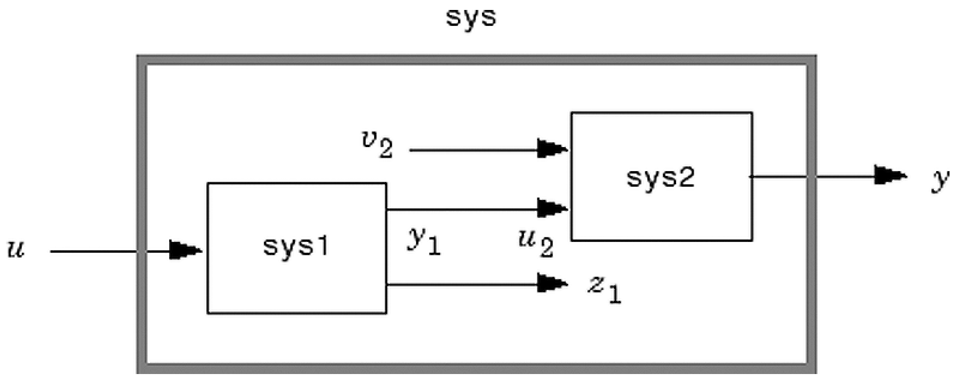
Series 2: Connect the AHP model sys1 and the queuing theory model sys2 in series according to the following instructions: sys = series (sys1, sys2), to form a basic series connection as shown below in Figure 4, where u is the input data and y is the output data:
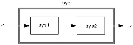
Figure 4.
The analytic hierarchy process and the queuing theory model in series.
This command is equivalent to direct multiplication: sys = sys2 * sys1;
Through the above two-step MATLAB instructions, the three models can be arranged in series, the data can be input and processed in sequence, and finally an order data chain can be arranged to be produced, and then can be output.
2.1. Step 1—Linear Programming Model
Step 1 of the proposed decision-making process is based on a linear programming model that can maximize profit or minimize cost with limited resources, eliminating the profitless, not cost-effective, very low orders; second, the maximum profit value of each order as one of the important factors in the hierarchical analysis, will become, together with the delivery date and other factors in the next module, the hierarchical analysis. In production planning, linear programming models can be used to determine how many units of different products should be produced to maximize profits. The model is as follows:
Among them, x1 is the number of product type 1; c1 represents the profit of the first product; a11 is the consumption of the first resource in the first constraint condition; represents the total amount of the first resource; …, is the number of n products; represents the profit of the n type of product; is the consumption of the first resource in the M constraint condition; and represents the total amount of the M resources.
The MATLAB execution code is as follows:
- clc
- clear all
- c = [c1 c2 c3 c4 …… cn − 1 cn];
- a = [a11a12a13….a1n; a21a22a23 …. a2n; ……; am1 am2 am3 …. amn];
- b = [b1; b2; b3; ……; bm];
- aeq = [0];
- beq = [0];
- lb = [0;0;0];
- ub = [inf;inf;inf];
- [x,fval] = linprog(-c,a,b,aeq,beq,lb,ub);
- best = c*x%;
The result of step 1 is the calculation of the maximum profit of all orders, and the screening and deleting of low cost-effective orders (for example: orders with very low profits, long production cycle or orders with high wastage), while the calculated maximum profit will be used as important indicator factors for the hierarchical analysis.
2.2. Step 2—Analytic Hierarchy Process (AHP)
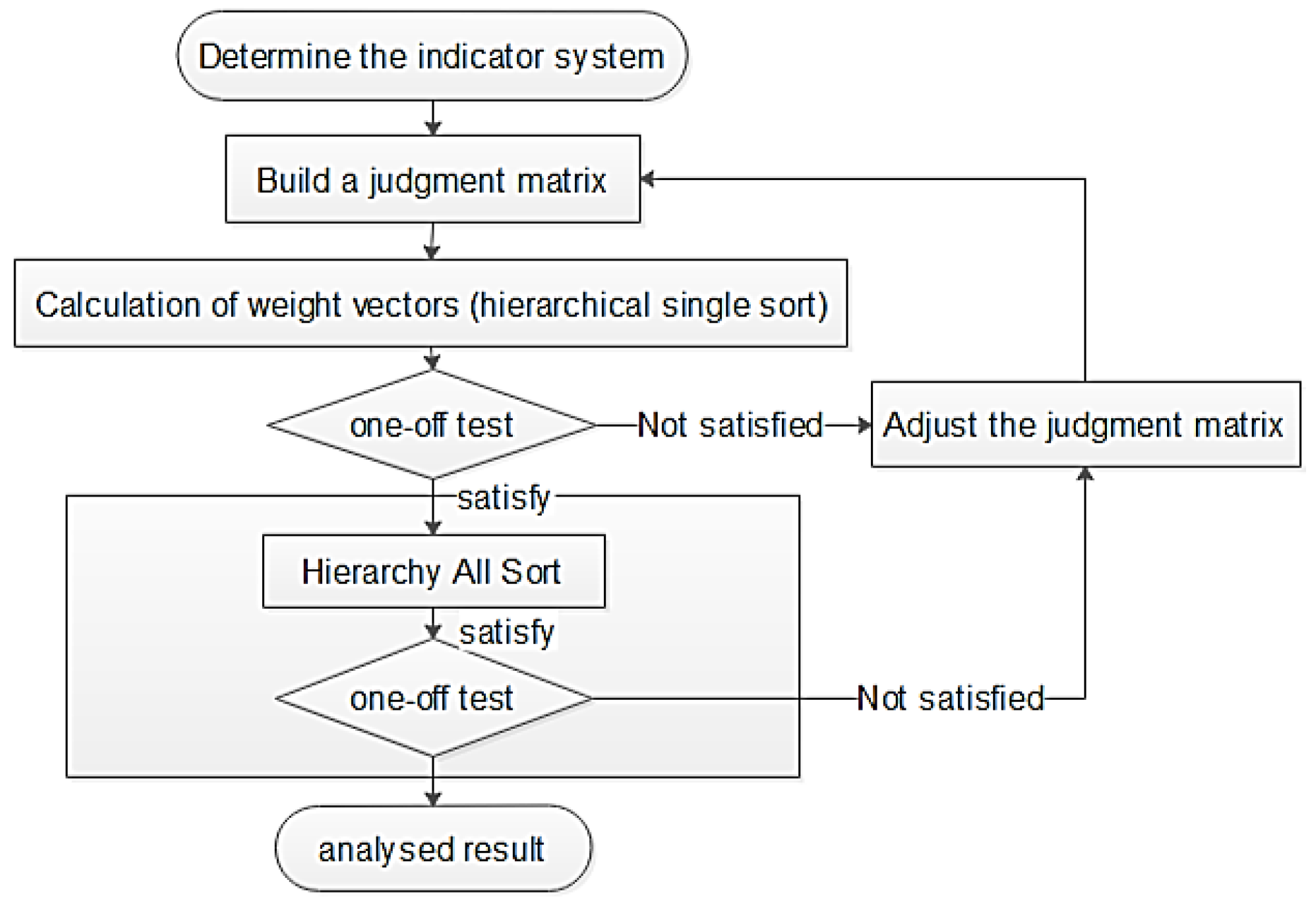
AHP mainly breaks down the influencing factors always related to decision-making into a target layer, criterion layer and scheme layer, hierarchizes and digitizes the influencing factors, and conducts qualitative analysis on this basis. Here is a detailed analysis of the analysis process of the analytic hierarchy process, including construction model and algorithm demonstration and MATLAB programming [6,11,13]. The analytical flow chart of analytic hierarchy process is presented in Figure 5:
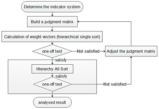
Figure 5.
Hierarchical analysis process flowchart.
The application process of the analytic hierarchy process mainly includes four steps:
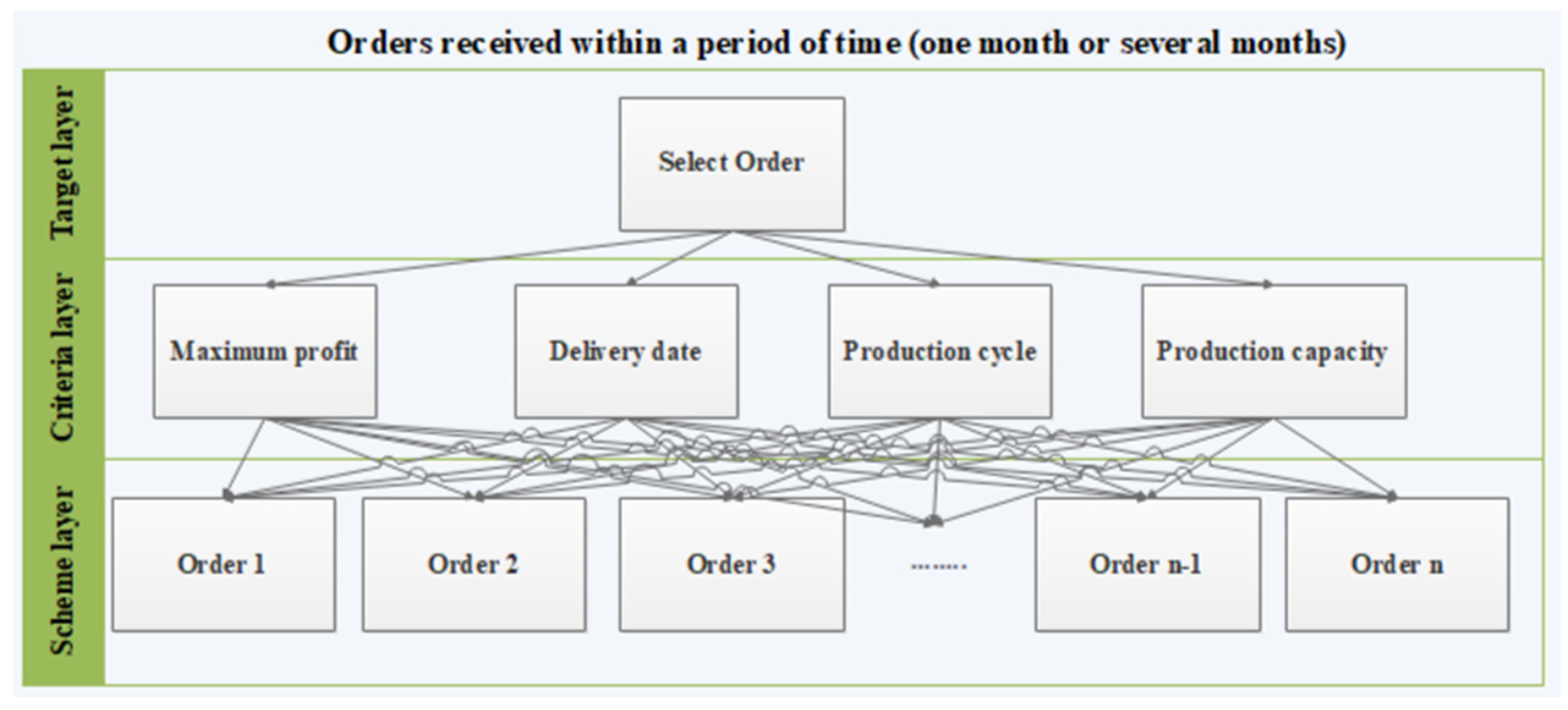
2.2.1. Construct the Hierarchical Structure Model
Target layer: Select priority production orders;
Criteria layer: Factors that influence decision-making include the maximum profit value of a single order, delivery date, and production cycle and production capacity;
Solution layer: various orders, determine the order production sequence as shown in Figure 6.
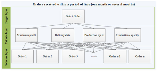
Figure 6.
Constructed model of hierarchical analysis.
2.2.2. Construct the Judgment Matrix
To construct a judgment matrix is to compare each element pairwise and determine the weight of each criterion layer to the target layer. It is to compare and judge the index of the criterion layer pairwise [12]. Usually we use Santy’s 1–9 scale method to give the following implications as shown in Table 1:

Table 1.
Santy’s 1–9 scale.
For the criterion layer, which we call A, we can build:
where the element of A is satisfied:
For example, for the criterion layer: maximum profit, production cycle, delivery date, production capacity, we can construct such a 4 × 4 judgment matrix; how is presented in Table 2:
Table 2.
The studied case.
The diagonal line is defined for each indicator according to Santy’s 1–9 scale method, as well as the focus of the manufacturing enterprise and so on until a complete judgment matrix is constructed.
2.2.3. Enter the Judgment Matrix A and Find the Weights and MATLAB Code
Process 1: Normalization of the judgment matrix:
Process 2: Add the processed judgment matrix by row
Process 3: Normalize the vector :
Then is the desired eigenvector, and in hierarchical single ordering, is the weight of index to indexV.
The MATLAB code:
- Sum_A =sum(A)
- [n,n] =size(A)
- SUM_A = repmat(Sum_A,n,1)
- Stand_A = A./SUM_A
- sum(Stand_A,2)
- disp(sum(Stand_A,2)/n)
2.2.4. Consistency Detection
Process 1: Calculate the consistency index CI:
Process 2: Find the corresponding average random consistency index RI table;
Process 3: Calculate the consistency ratio CR:
The MATLAB code for consistency checking is as follows:
CI = (Max_eig − n)/(n − 1);
RI = [………………………];
CR = CI/RI(n);
if CR < 0.10
disp(“CR < 0.10”)
else
disp(“CR >= 0.10”)
end
Note:
- If CR < 0.10, the consistency of the judgment matrix is acceptable;
- If CR ≥ 0.10, the judgment matrix needs to be modified in step 2.
It can be concluded that step 2 uses the four index factors of the Analytical Hierarchy Process to hierarchically arrange the production order of the orders. Finally, we get an orderly order chain. According to the rules of priority production, arrange the order chain and enter step 3.
2.3. Step 3—Queuing Theory Calculation
Queuing theory uses the statistical study of service orders and service time to obtain the statistical rules of quantity indicators (waiting time, queue length, busy period), and then, according to these rules, to improve the structure of the service system or reorganize the service object, so that the service system can meet the needs of the service object.
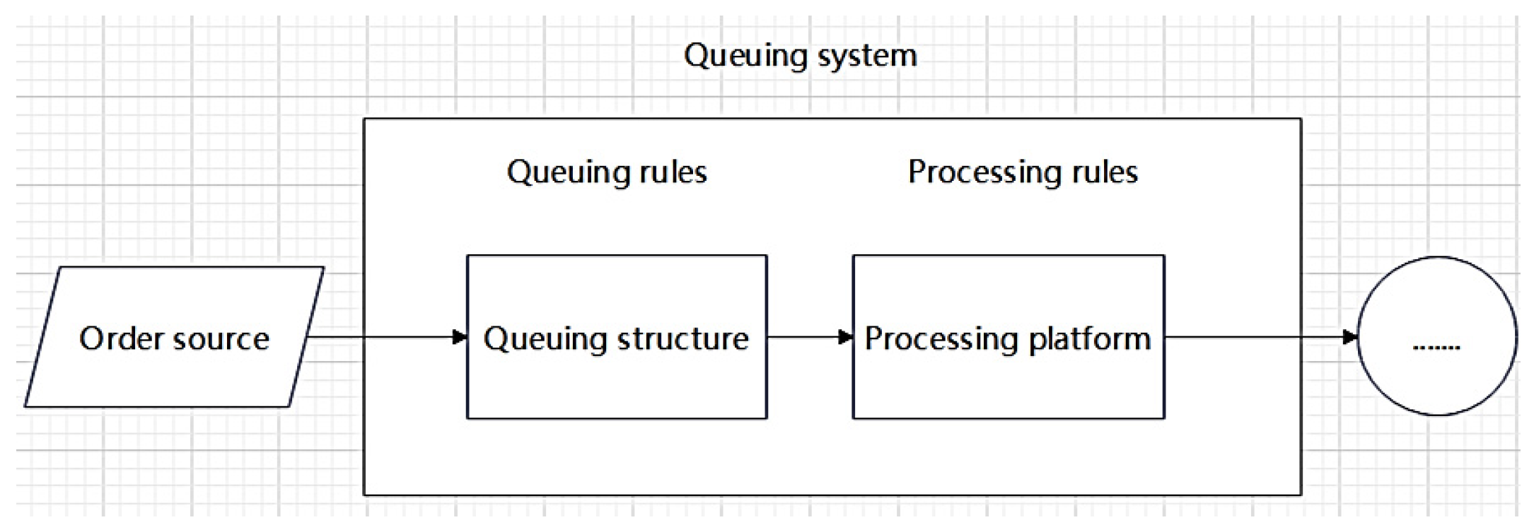
2.3.1. Queuing Process
It can also make the cost of the institution the most economical or some indicators the best that they can be as shown in Figure 7.
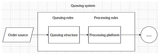
Figure 7.
Queuing process.
2.3.2. Derive Model M/M/S/∞/∞/PR from Model M/M/1/∞/∞/PR
Here, we mainly demonstrate the derivation of the index formula of queuing theory and MATLAB code, and show you how to use queuing theory to improve the production efficiency of manufacturing factories, so that the cost of institutions is the most economical or some indicators are optimal. We use an M/M/1/∞/∞/PR queueing theory model to demonstrate the process formula derivation:
- Mode l: M/M/1/∞/∞/PR
- The first M shows that the arrival process of the order workpiece follows Poisson flow or that the arrival interval of the order workpiece follows a negative exponential distribution;
- The second M means that the service time is subject to negative exponential distribution;
- 1 indicates 1 workbench;
- The first ∞ means that the system service capacity is unlimited;
- The second ∞ means that the source of the order artifact is unlimited;
- PR stands for priority service;
Demonstration of the derivation process:
- Assumption: The average workpiece arrival rate per unit time is λ
- The average service rate of the workbench per unit time is μ
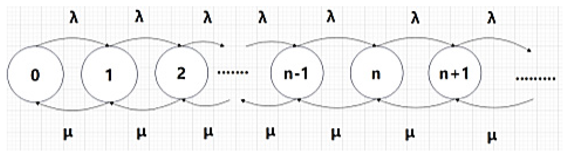
Therefore, the most important thing for us is to find the probability of n workpieces in the system, and the key is to find the equilibrium of the state and solve the equation according to the equilibrium of the state. For the state equilibrium equation diagram look at Figure 8:
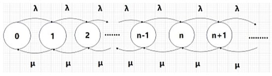
Figure 8.
Equilibrium equation of state.
- 0 means that there are 0 workpieces in the system with, a probability of P0;
- 1 means that there is 1 workpiece in the system, with a probability of P1;
- n means that there are n workpieces in the system, with a probability of Pn.
The inflow rate in each state is , that is, the arrival rate per workpiece is . Because there is only one workbench, the workpiece departure rate in each state is also equal to the average service rate , so as to solve the equilibrium equation of the state. The equilibrium equation of states is that in any state, the total inflow rate of state n is equal to its outflow rate.
where It is the level of prosperity or utilization ratio of the system
So:
Process 1. State probability :
This is a geometric sequence, =, =, (n→∞); the formula for finding the sum of n terms in a geometric sequence:
We know , must be less than 1, (); because is not less than 1, the term of this system will continue to extend without end, resulting in overloaded work, which is impossible in actual production, so we only consider the condition of .
Because: = 1.
The probability that there are no workpieces in the system is: =.
So, the probability that there are n workpieces in the system is:
Process 2. Line length L:
The line length is the expected value; L is equal to the number of pieces in each state × the probability of each state:
Next, we will calculate the queue length , the average residence time of the workpiece W, and the average waiting time of the workpiece according to the existing Little formula of the queue theory:
Process 3. The queue length :
Process 4. The average residence time of the workpiece W:
Process 5. The average waiting time of the workpiece :
- Model 2: M/M/S/∞/∞/PR
The difference between model 2 and model 1 is that there are S service desks. The work of each service desk is independent of each other, and the service rate is equal. If the S service desks are busy when the customer arrives, the workpieces will be queued up to wait, as a single-team model with priority service.
Average service rate of the entire system: S,p* (p* < 1). It can replace with p* and recalculate it by bringing it into the formula of Model 1, which will not be shown in detail here. Here is a detailed demonstration of the running code using MATLAB code:
- s = n;
- mu = x;
- lambda = y;
- ro = lambda/mu;
- ros = ro/s;
- sum1 = 0;
- for i = 0:(s − 1)
- sum1 = sum1 + ro.^i/factorial(i);
- end
- sum2 = ro.^s/factorial(s)/(1 − ros);
- p0 = 1/(sum1+sum2);
- p = ro.^s.*p0/factorial(s)/(1 − ros);
- Lq = p.*ros/(1 − ros);
- L = Lq + ro;
- W = L/lambda;
- Wq = Lq/lambda;
Through all the formulas calculated above, the final result of all formulas is the average workpiece arrival rate per unit time, and the average service rate of the workbench per unit time is . By controlling and adjusting the frequency of and , we conduct statistical research on service orders and service time and obtain statistical rules for quantity indicators.
Then, according to these rules, we improve the structure of the service system or reorganize the order, and carry out decision-making, scheduling and production, so that the service system can meet the needs of the order. At the same time, the cost of manufacturing enterprises is the most economical or some indicators are optimized.
The advantage of this decision-making system is that it uses existing software to perform combined operations on mathematical models, which has pertinence, ow-cost, is easily operable and has obvious effects. It can help companies maximize profits, improve production efficiency, and meet customer demand for order adjustments, which be more adaptable to the fiercely competitive market and changing environment.
3. Conclusions
The combination of the linear programming model, analytic hierarchy process (AHP) and queuing theory model can effectively solve the problems of production chaos, low production efficiency and the inability of manufacturing enterprises to obtain maximum profits from limited resources in decision scheduling.
The combined model has good profitability and the ability to solve customer needs in real time, repeatably. There are great improvements and innovations in flexibility, reliability and robustness, which can help manufacturing enterprises to obtain maximum profits. This can improve decision management and production mode, improve production efficiency, ensure production schedules, meet customer needs and improve satisfaction.
However, the combination model also has certain limitations, which are due to the connection between the models themselves, which is inevitable, so there is no best model, only a better model. At present, the development of the manufacturing industry is still plagued by the application and popularization of various technologies, but in the future, with the mature combination and popularization of AI technology, Internet of Things, big data and cloud computing, the manufacturing industry will have stronger decision-making, management, scheduling and profitability.
In the future, our work will focus on the application of artificial intelligence and big data technology, and even Internet of Things technologies, in the decision-making system. However, since the current development and maturity of these technologies have not reached universalization, this will be an important challenge for future work.
Author Contributions
Conceptualization, G.B. and P.V.; methodology, G.B.; software, G.B.; investigation, G.B.; data curation, G.B.; writing—original draft preparation, G.B.; writing—review and editing, P.V.; visualization, G.B.; supervision, P.V.; project administration, P.V.; funding acquisition, P.V. All authors have read and agreed to the published version of the manuscript.
Funding
This publication was financed under project number 24-BM-01 “Researching the challenges and perspectives for Bulgarian organizations in the context of economic digitalization and internationalization”, carried out by the National Scientific Research Fund of Bulgaria and the University of Ruse.
Institutional Review Board Statement
Not applicable.
Informed Consent Statement
Not applicable.
Data Availability Statement
No new data were created or analyzed in this study. Data sharing is not applicable to this article.
Conflicts of Interest
The author declares no conflicts of interest.
References
- Elbasheer, M.; Longo, F.; Nicoletti, L.; Padovano, A.; Solina, V.; Vetrano, M. Applications of ML/AI for Decision-Intensive Tasks in Production Planning and Contro. Procedia Comput. Sci. 2022, 200, 1903–1912. [Google Scholar] [CrossRef]
- Gao, Q.; Cheng, C.; Sun, G. Big data application, factor allocation, and green innovation. Chin. Manuf. Enterp. 2023, 192, 122567. [Google Scholar]
- Long, G.; Lin, B.; Cai, H.; Nong, G. Developing an Artificial Intelligence (AI) Management System to Improve Product Quality and Production Efficiency. Furnit. Manuf. Procedia Comput. Sci. 2020, 166, 486–490. [Google Scholar] [CrossRef]
- Vitliemov, P.; Stoycheva, B. Technology solutions and challenges for innovations that will improve our lives in pandemic crisis. AIP Conf. Proc. 2022, 2449, 070007. [Google Scholar] [CrossRef]
- Azeem, M.; Haleem, A.; Bahl, S.; Javaid, M.; Suman, R.; Nandan, D. Big data applications to take up major challenges across manufacturing industries: A brief review. Mater. Today: Proc. 2020, 49, 339–348. [Google Scholar] [CrossRef]
- Li, C.; Chen, Y.; Chang, Y. A review of industrial big data for decision making in intelligent manufacturing, Engineering Science and Technology. Int. J. 2022, 29, 101021. [Google Scholar]
- Corallo, A.; Crespino, A.M.; Lazoi, M.; Lezzi, M. Model-based Big Data Analytics-as-a-Service framework in smart manufacturing: A case study. Robot. Comput.-Integr. Manuf. 2022, 76, 102331. [Google Scholar] [CrossRef]
- Mei, L.; Yue, L.; Ge, S. Joint decision-making of virtual module formation and scheduling considering queuing time. Data Sci. Manag. 2023, 6, 134–143. [Google Scholar] [CrossRef]
- Seenivasan, M.; Senthilkumar, R.; Subasri, K.S. M/M/2 heterogeneous queueing system having unreliable server with catastrophes and restoration. Mater. Today: Proc. 2022, 51, 2332–2338. [Google Scholar] [CrossRef]
- Wang, Y.; Xia, T.; Xu, X.; Ding, Y.; Zheng, M.; Pan, E.; Xi, L. Joint optimization of flexible job shop scheduling and preventive maintenance under high-frequency production switching. Int. J. Prod. Econ. 2024, 269, 109163. [Google Scholar] [CrossRef]
- Zhou, B.; Bao, J.; Li, J.; Lu, Y.; Liu, T.; Zhang, Q. A novel knowledge graph-based optimization approach for resource allocation in discrete manufacturing workshops. Robot. Comput. -Integr. Manuf. 2021, 71, 102160. [Google Scholar] [CrossRef]
- Hanukov, G. A queueing-inventory system in which customers can orbit during the service. IFAC Pap. 2022, 55, 619–624. [Google Scholar] [CrossRef]
- Vafaei, N.; Delgado-Gomes, V.; Agostinho, C.; Jardim, R. Analysis of Data Normalization in Decision Making Process for ICU’s Patients During the Pandemic. Procedia Comput. Sci. 2022, 214, 809–816. [Google Scholar] [CrossRef]

Disclaimer/Publisher’s Note: The statements, opinions and data contained in all publications are solely those of the individual author(s) and contributor(s) and not of MDPI and/or the editor(s). MDPI and/or the editor(s) disclaim responsibility for any injury to people or property resulting from any ideas, methods, instructions or products referred to in the content. |
© 2024 by the authors. Licensee MDPI, Basel, Switzerland. This article is an open access article distributed under the terms and conditions of the Creative Commons Attribution (CC BY) license (https://creativecommons.org/licenses/by/4.0/).