
Procedure for Verifying Population Exposure Limits to the Magnetic Field from Double-Circuit Overhead Power Lines


Abstract
:1. Introduction
2. Calculation of Exposure to the Magnetic Field Generated by Power Lines
- Infinite plane terrain having a relative permeability ;
- line conductors, straight, parallel, and having infinite length;
- balanced set of line currents.
2.1. Single-Circuit Lines
2.2. Double-Circuit Lines
3. Proposed Calculation Procedure
3.1. Single-Circuit Lines
3.2. Double-Circuit Lines
3.3. Procedure Sum up and Discussion
Possible Extensions of the Proposed Method
4. Validation of the Proposed Method on a Medium Voltage Double-Circuit Line
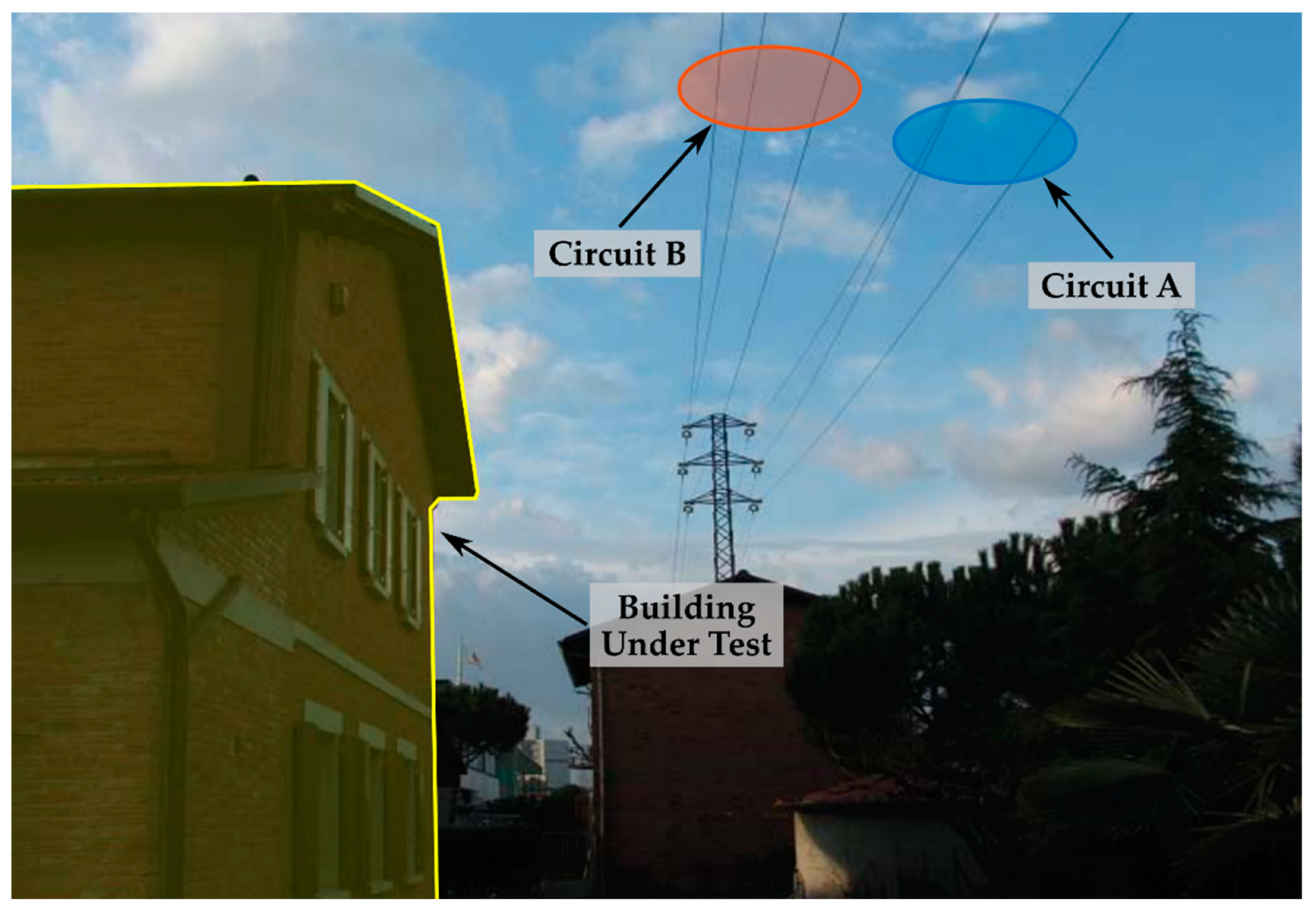
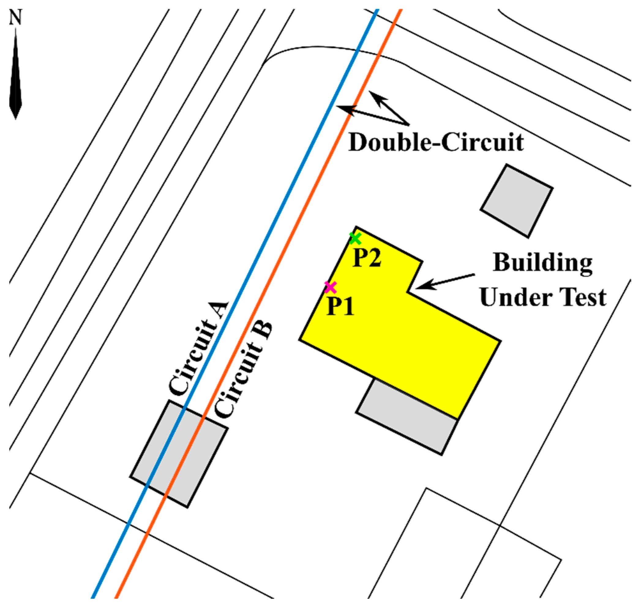
4.1. Building under Test
- Medium voltage (15 kV) double-circuit overhead power line adjacent to the building under consideration (see Figure 2), which is the primary field source, consisting of circuit A (displayed in blue color) and circuit B (displayed in orange color);
- Nearby distribution substation (not displayed);
- Three further medium-voltage lines are derived from the distribution substation.
- Circuit A: overhead power line with a conductor section of 70 mm2 and thermal limit equal to 285 A;
- Circuit B: overhead power line with a conductor section of 50 mm2 and thermal limit equal to 230 A;
4.2. Current Regulatory Framework
- Italian nationwide law: the Decree of The President of The Council of Ministers DPCM 8 July 2003 sets exposure limit to 100 μT, attention value 10 μT, and quality target 3 μT [12]. Concerning limits set by [12], measurement guidelines are reported in the CEI 106-11:2006 standard [32]. Occupational users’ are regulated at the European level by 2013/35/EU [33];
- Emilia-Romagna law: although the region Emilia-Romagna is currently applying nationwide laws, in the first 2000s, magnetic field regulatory values for new buildings were set to an exposure limit of 100 μT, caution value 0.5 μT, and quality target 0.2 μT (similarly to what still applies in Brussels and Flanders area). Exposure values should be evaluated assuming 5% higher than the average current experienced by the line in the previous year or, if more precautionary, 50% of the line rated current;
- ICNIRP limits: field values are set to 500 μT for occupational users’ exposure and 100 μT for general public exposure [6];
- IEEE and NATO recommendations: Head and torso should not overpass 904 μT and 2.71 mT in unrestricted and restricted environments, respectively. On the other hand, limb exposure is limited to 75.8 mT for all the environments. Further details are available in IEEE Std C95.1-2019 [14].
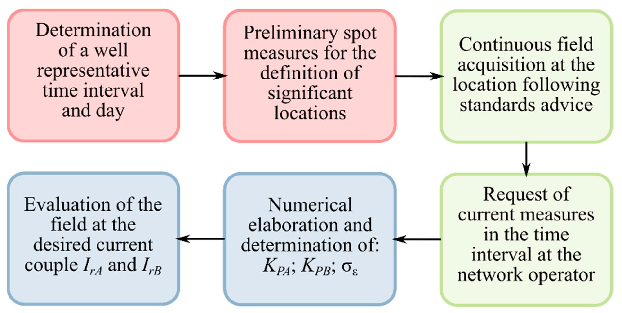
4.3. Description of the Measurement Procedure
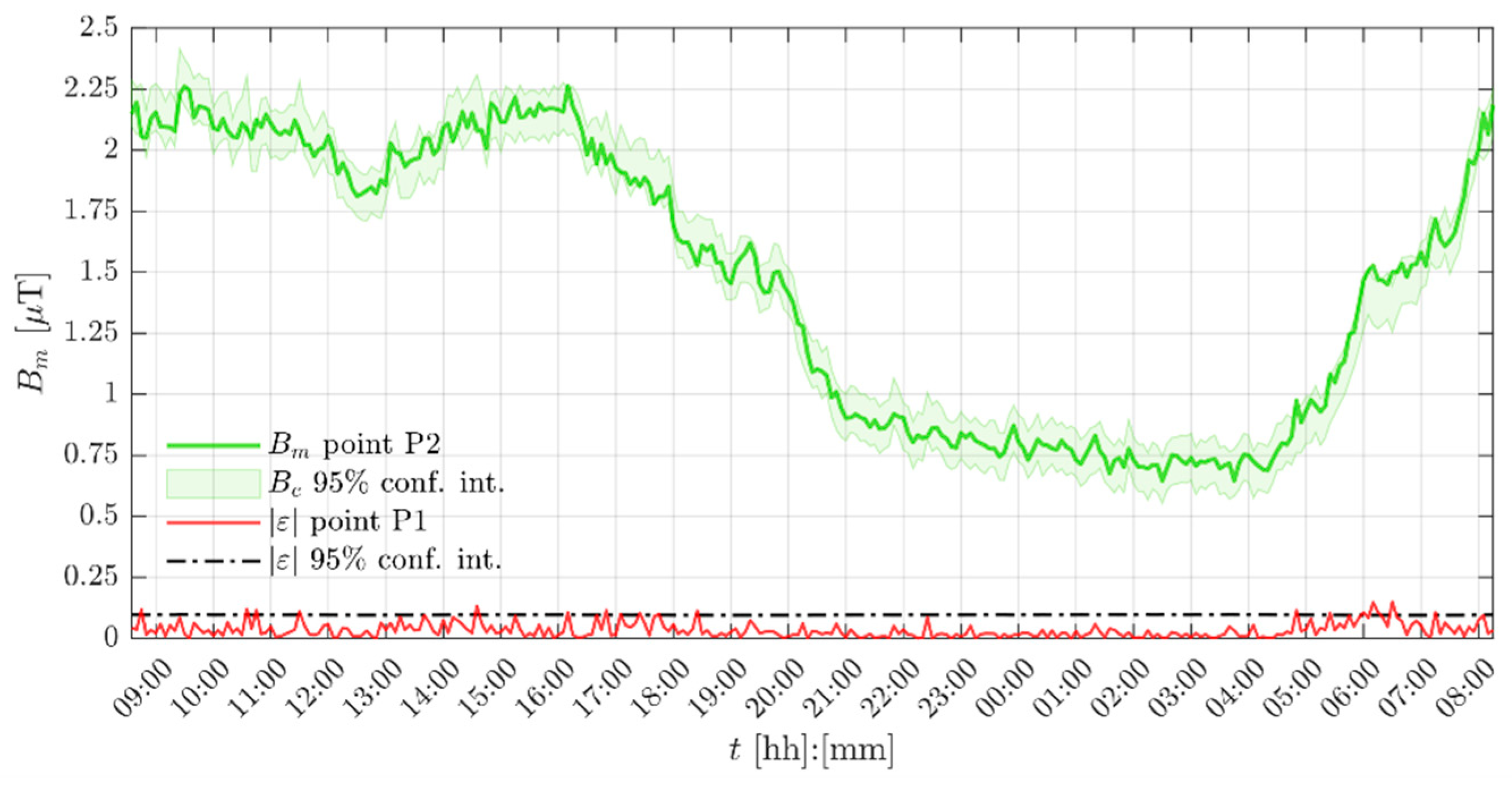
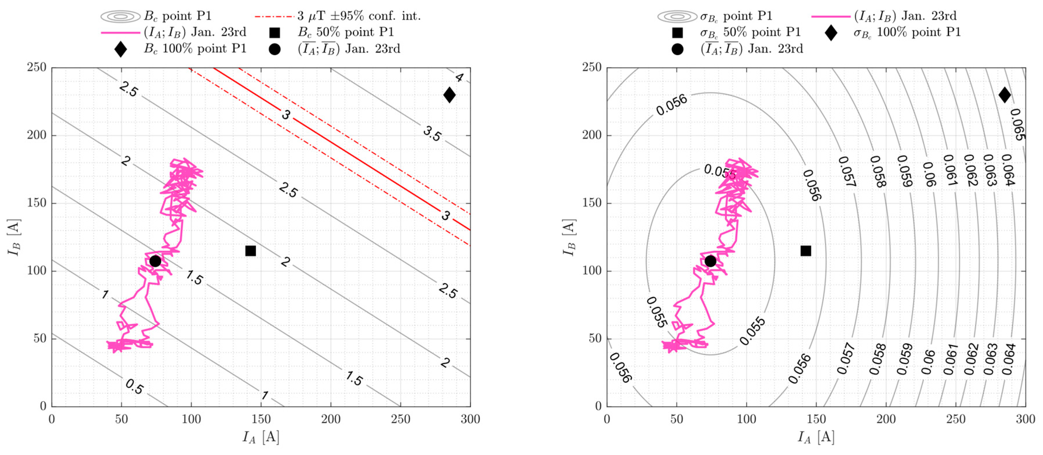
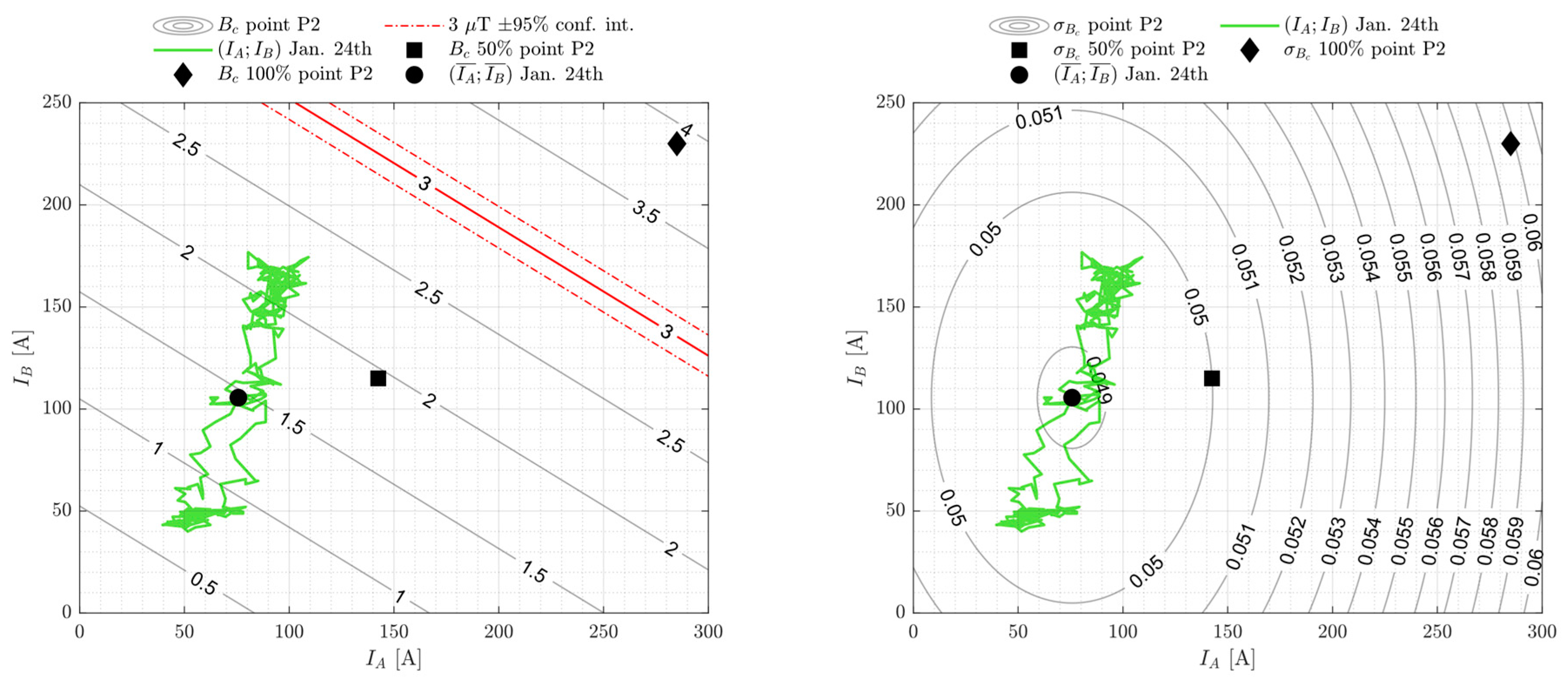
4.4. Measurements Processing Using the Proposed Procedure
4.5. Evaluation of the Magnetic Field Exposure
5. Conclusions
Author Contributions
Funding
Institutional Review Board Statement
Informed Consent Statement
Data Availability Statement
Conflicts of Interest
References
- Bendík, J.; Cenký, M.; Eleschová, Ž.; Beláň, A.; Cintula, B.; Janiga, P. Comparison of electromagnetic fields emitted by typical overhead power line towers. Electr. Eng. 2020, 1–12. [Google Scholar] [CrossRef]
- Woodside, G.; Kocurek, D.S. Environmental, Safety, and Health Engineering; Wiley: Hoboken, NJ, USA, 1997; ISBN 978-0-471-10932-7. [Google Scholar]
- Olsen, R.G. High Voltage Overhead Transmission Line Electromagnetics; CreateSpace: Scotts Valley, CA, USA, 2018; Volume 2, ISBN 978-1507848043. [Google Scholar]
- IARC. Non-Ionizing Radiation, Part 1: Static and Extremely Low-frequency (ELF) Electric and Magnetic Fields; IARC Publications: Lyon, France, 2002; ISBN 978-92-832-1280-6. [Google Scholar]
- WHO. Establishing a Dialogue on Risks from Electromagnetic Fields; World Health Organization: Geneva, Switzerland, 2002. [Google Scholar]
- International Commission on Non-Ionizing Radiation Protection. Guidelines for limiting exposure to time-varying electric, magnetic, and electromagnetic fields (up to 300 GHz). Health Phys. 1998, 74, 494–522. [Google Scholar]
- CIGRE Working Group C3.19. Responsible Management of Electric and Magnetic Fields (EMF); CIGRE Technical Brochure 806, Electra 311; CIGRE: Paris, France, 2020. [Google Scholar]
- Tuominen, M.; Olsen, R. Electrical design parameters of all-dielectric-self-supporting fiber optic cable. IEEE Trans. Power Deliv. 2000, 15, 940–947. [Google Scholar] [CrossRef]
- Schutt, A.J. The Power Line Dilemma: Compensation for Diminished Property Value Caused by Fear of Electromagnetic Fields. Fla. State Univ. Law Rev. 1996, 24, 125. [Google Scholar]
- Stam, R. Comparison of International Policies on Electromagnetic Fields; National Institute of Public Health and Environment: Bilthoven, The Netherlands, 2018. [Google Scholar]
- Publications Office of the EU. 1999/519/EC: Council Recommendation of 12 July 1999 on the Limitation of Exposure of the General Public to Electromagnetic Fields (0 Hz to 300 GHz). Available online: https://op.europa.eu/en/publication-detail/-/publication/9509b04f-1df0-4221-bfa2-c7af77975556/language-en (accessed on 20 May 2021).
- Gazzetta Ufficiale Della Republica Italiana. DPCM 8 luglio 2003—Fissazione Dei Limiti DI Esposizione, Dei Valori DI Attenzione E Degli Obiettivi DI Qualità per la Protezione Della Popolazione Dalle Esposizioni AI Campi Elettrici E Magnetici Alla Frequenza DI Rete (50 Hz) Generati Dagli Elettrodotti. Available online: https://www.gazzettaufficiale.it/eli/id/2003/08/29/03A09749/sg (accessed on 18 May 2021). (In Italian).
- Ranković, A. Novel multi-objective optimization method of electric and magnetic field emissions from double-circuit overhead power line. Int. Trans. Electr. Energy Syst. 2017, 27, 1–22. [Google Scholar] [CrossRef]
- Institute of Electrical and Electronics Engineers. IEEE Std C95.1-2019—IEEE Standard for Safety Levels with Respect to Human Exposure to Electric, Magnetic, and Electromagnetic Fields, 0 Hz to 300 GHz; Institute of Electrical and Electronics Engineers: Piscataway, NJ, USA, 2019; pp. 1–312. [Google Scholar] [CrossRef]
- Deltuva, R.; Lukočius, R. Distribution of Magnetic Field in 400 kV Double-Circuit Transmission Lines. Appl. Sci. 2020, 10, 3266. [Google Scholar] [CrossRef]
- Mazzanti, G. The Role Played by Current Phase Shift on Magnetic Field Established by AC Double-Circuit Overhead Transmission Lines—Part I: Static Analysis. IEEE Trans. Power Deliv. 2006, 21, 939–948. [Google Scholar] [CrossRef]
- Mazzanti, G. The Role Played by Current Phase Shift on Magnetic Field Established by Double-Circuit Overhead Transmission Lines—Part II: Dynamic Analysis. IEEE Trans. Power Deliv. 2006, 21, 949–958. [Google Scholar] [CrossRef]
- Ponnle, A.; Adedeji, K.; Abe, B.; Jimoh, A. Spatial magnetic field polarization below balanced double-circuit linear configured power lines for six phase arrangements. In Proceedings of the 2015 Intl Aegean Conference on Electrical Machines Power Electronics (ACEMP), 2015 Intl Conference on Optimization of Electrical Electronic Equipment (OPTIM) 2015 Intl Symposium on Advanced Electromechanical Motion Systems (ELECTROMOTION), Side, Turkey, 2–4 September 2015; pp. 163–169. [Google Scholar]
- Landini, M.; Mazzanti, G.; Sandrolini, L.; D’Adda, F. A Novel Algorithm for the 3D Calculation of the Magnetic Field Generated by Complex Configurations of Overhead Power Lines. In Proceedings of the 2019 IEEE International Conference on Environment and Electrical Engineering and 2019 IEEE Industrial and Commercial Power Systems Europe (EEEIC/I&CPS Europe), Genova, Italy, 11–14 June 2019; pp. 1–4. [Google Scholar]
- Dahab, A.; Amoura, F.; Abu Elhaija, W. Comparison of Magnetic-Field Distribution of Noncompact and Compact Parallel Transmission-Line Configurations. IEEE Trans. Power Deliv. 2005, 20, 2114–2118. [Google Scholar] [CrossRef]
- Khaled Omar Basharahil, M.; Azlinda Ahmad, N. Electromagnetic Fields Characteristics From Overhead Lines, Underground Cables and Transformers Determined Using Finite Element Method. In Proceedings of the 2021 IEEE International Conference on the Properties and Applications of Dielectric Materials (ICPADM), Johor Bahru, Malaysia, 12–14 July 2021; pp. 338–341. [Google Scholar]
- Shiina, T.; Kudo, T.; Herai, D.; Kuranari, Y.; Sekiba, Y.; Yamazaki, K. Calculation of Internal Electric Fields Induced by Power Frequency Magnetic Fields During Live-Line Working Using Human Models With Realistic Postures. IEEE Trans. Electromagn. Compat. 2021, 1–8. [Google Scholar] [CrossRef]
- Lunca, E.; Istrate, M.; Salceanu, A.; Tibuliac, S. Computation of the magnetic field exposure from 110 kV overhead power lines. In Proceedings of the EPE 2012—Proceedings of the 2012 International Conference and Exposition on Electrical and Power Engineering, Iasi, Romania, 25–27 October 2012; pp. 628–631. [Google Scholar]
- Mazzanti, G.; Landini, M.; Kandia, E. A Simple Innovative Method to Calculate the Magnetic Field Generated by Twisted Three-Phase Power Cables. IEEE Trans. Power Deliv. 2010, 25, 2646–2654. [Google Scholar] [CrossRef]
- Mazzanti, G.; Landini, M.; Kandia, E.; Bernabei, A.; Cavallina, M. Magnetic Field Generated by Double-Circuit Twisted Three-Phase Cable Lines. Prog. Electromagn. Res. C 2017, 73, 115–126. [Google Scholar] [CrossRef] [Green Version]
- Harun, Z.A.; Osman, M.; Ariffin, A.M.; Zainal Abidin Ab Kadir, M. Effect of AC Interference on HV Underground Cables Buried Within Transmission Lines Right of Way. In Proceedings of the 2021 IEEE International Conference on the Properties and Applications of Dielectric Materials (ICPADM), Johor Bahru, Malaysia, 12–14 July 2021; pp. 73–76. [Google Scholar]
- SAI Global. CEI 211-4—Guide to Calculation Methods of Electric and Magnetic Fields Generated by Power-Lines and Electrical Substations. Available online: https://i2.saiglobal.com/management/display/anchor/346715/-/83253acef73050bb25f13edf9a274b1d (accessed on 18 April 2021).
- ISO. ISO—17.220.20—Measurement of Electrical and Magnetic Quantities. Available online: https://www.iso.org/ics/17.220.20/x/ (accessed on 18 April 2021).
- Mazzanti, G. Uncertainties in the calculation of continuous exposure of general public to magnetic field from ac overhead transmission lines. In Proceedings of the IEEE Power Engineering Society General Meeting, San Francisco, CA, USA, 16 June 2005; Volume 3, pp. 2583–2590. [Google Scholar]
- Benes, M.; Comelli, M.; Bampo, A.; Villalta, R. Procedure di misura di campi elf in prossimità di configurazioni complesse di linee elettriche. In Proceedings of the AIRP—Convegno Nazionale di Radioprotezione, Catania, Italy, 15–17 September 2005; pp. 1–6. [Google Scholar]
- Andreuccetti, D.; Zoppetti, N.; Fanelli, N.; Giorgi, A.; Rendina, R. Magnetic fields from overhead power lines: Advanced prediction techniques for environmental impact assessment and support to design. In Proceedings of the 2003 IEEE Bologna Power Tech Conference Proceedings, Bologna, Italy, 23–26 June 2003; Volume 2, pp. 1009–1015. [Google Scholar]
- SAI Global. CEI 106-11—Guide for the Determination of the Respect Widths for Power Lines and Substations According to DPCM 8 July 2003 (Clause 6)—Part 1: Overhead Lines and Cables. Available online: https://i2.saiglobal.com/management/display/index/0/671694/-/79c654e525e1d90a0a4301ab29a3682f (accessed on 1 September 2021).
- EUR-Lex. Directive 2013/35/EU of the European Parliament and of the Council of 26 June 2013 on the Minimum Health and Safety Requirements Regarding the Exposure of Workers to the Risks Arising from Physical Agents (Electromagnetic Fields) 20th Individual Directiv. Available online: https://eur-lex.europa.eu/legal-content/EN/TXT/?uri=CELEX%3A32013L0035 (accessed on 20 April 2021).
- SAI Global. CEI 211-6—Guide for the Measurement and the Evaluation of Electric and Magnetic Fields in the Frequency Range 0 Hz–10 Khz, with Reference to the Human Exposure. Available online: https://eu.i2.saiglobal.com/management/display/index/0/346796/-/1aa8ad8d2af832b947bb25ee87e9204c (accessed on 18 April 2021).
- SAI Global. IEC 61786-2:2014—Measurement of DC Magnetic, AC Magnetic and AC Electric Fields from 1 Hz to 100 kHz with Regard to Exposure of Human Beings—Part 2: Basic Standard for Measurements. Available online: https://webstore.iec.ch/publication/5907 (accessed on 1 September 2021).
- SAI Global. IEC 62110:2009—Electric and Magnetic Field Levels Generated by AC Power Systems—Measurement Procedures with Regard to Public Exposure. Available online: https://webstore.iec.ch/publication/6473 (accessed on 25 August 2021).
- IEEE Standards. 644-2019 (Revision IEEE Std 644-2008)—IEEE Standard Procedures for Measurement of Power Frequency Electric and Magnetic Fields from AC Power Lines; IEEE Standards Association: Piscataway, NJ, USA, 2020; pp. 1–40. [Google Scholar] [CrossRef]
- SAI Global. IEC 61786-1:2013—Measurement of DC Magnetic, AC Magnetic and AC Electric Fields from 1 Hz to 100 kHz with Regard to Exposure of Human Beings—Part 1: Requirements for Measuring Instruments. Available online: https://webstore.iec.ch/publication/5906 (accessed on 1 September 2021).
- IEEE Standards. 1308-1994—IEEE Recommended Practice for Instrumentation: Specifications for Magnetic Flux Density and Electric Field Strength Meters—10 Hz to 3 kHz; IEEE Standards Association: Piscataway, NJ, USA, 2020. [Google Scholar] [CrossRef]
- Gazzetta Ufficiale Della Republica Italiana. D.L. 18 Ottobre 2012, N. 179—Ulteriori Misure Urgenti per la Crescita Del Paese. Available online: https://www.gazzettaufficiale.it/eli/gu/2012/12/18/294/so/208/sg/pdf (accessed on 28 August 2021). (In Italian).


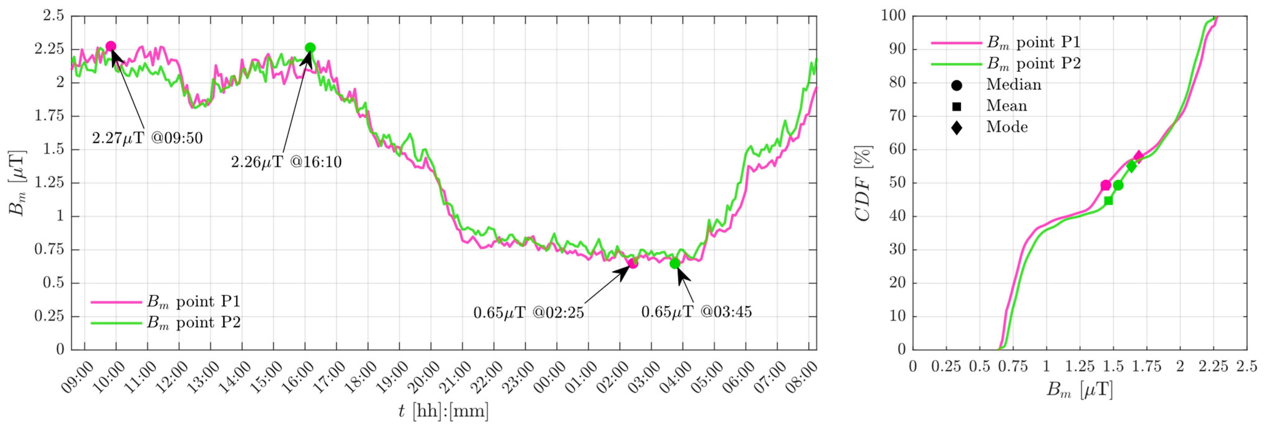
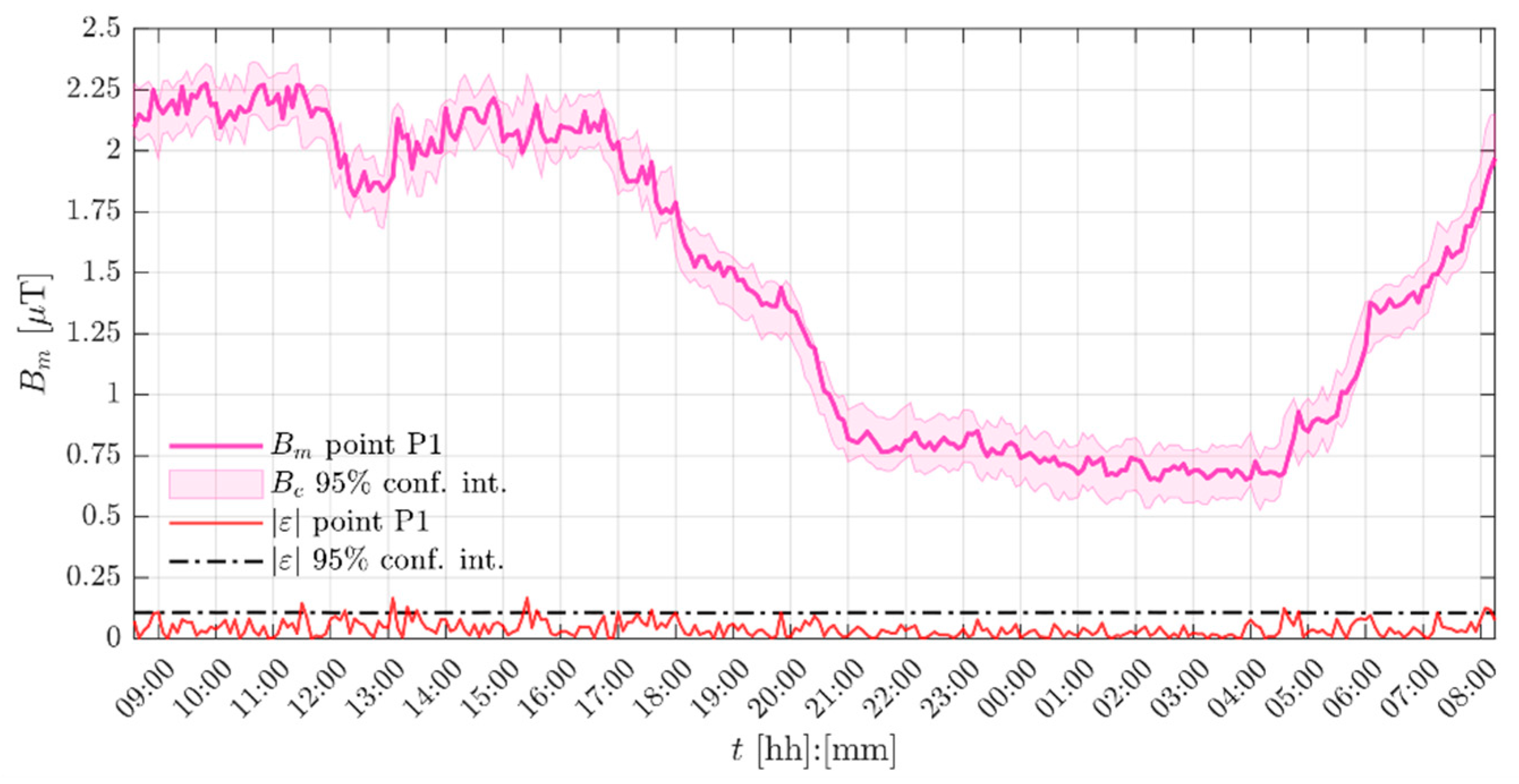
| Point | Mean [μT] | Median [μT] | Mode [μT] | Min. [μT] | Max. [μT] | Starting Day |
|---|---|---|---|---|---|---|
| P1 | 1.44 | 1.44 | 1.69 | 0.65 | 2.27 | 23rd of January |
| P2 | 1.46 | 1.54 | 1.63 | 0.65 | 2.26 | 24th of January |
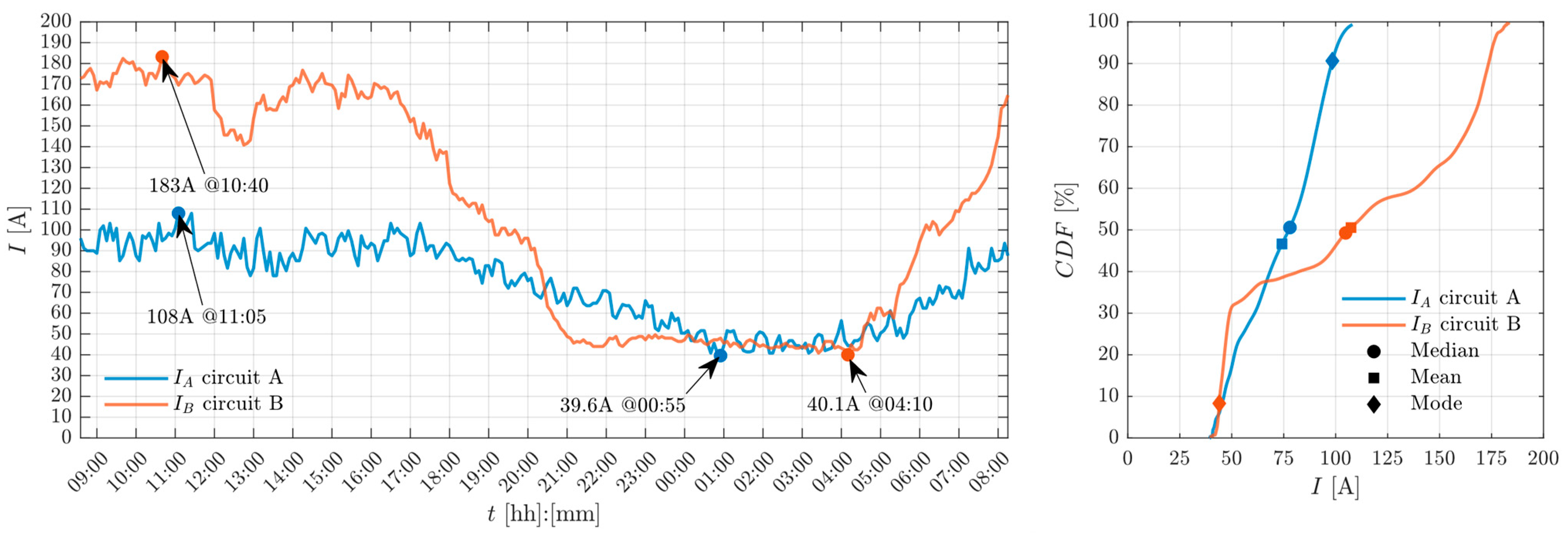
| Circuit | Mean [A] | Median [A] | Mode [A] | Min. [A] | Max. [A] | Starting Day |
|---|---|---|---|---|---|---|
| A | 74.2 | 78.1 | 98.4 | 39.6 | 108 | 23rd of January |
| 75.7 | 81 | 88.8 | 39.6 | 109 | 24th of January | |
| B | 107 | 105 | 43.9 | 40.1 | 183 | 23rd of January |
| 106 | 107 | 50.4 | 40.1 | 177 | 24th of January |
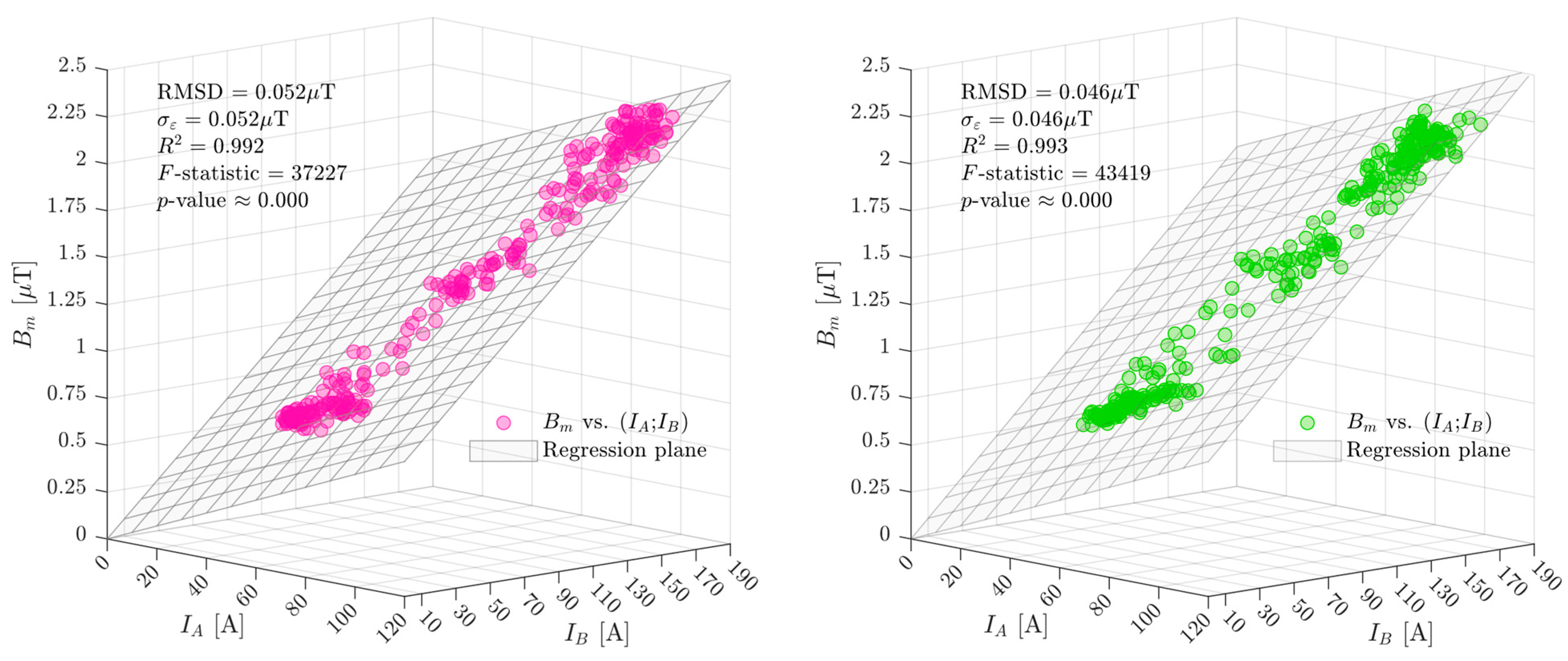
| Measurement Point | 95% Conf. Int. [μT/A] | 95% Conf. Int. [μT/A] | |||
|---|---|---|---|---|---|
| P1 | 0.0060 | 0.0060 ± 0.0003 | 0.0092 | 0.0092 ± 0.0002 | 0.052 |
| P2 | 0.0060 | 0.0060 ± 0.0003 | 0.0095 | 0.0095 ± 0.0002 | 0.046 |
| Measurement Point | Load | 95% Conf. Int. [μT] | |||
|---|---|---|---|---|---|
| P1 | 50% | 142.5 | 115.0 | 1.92 | 1.92 ± 0.11 |
| 100% | 285.0 | 230.0 | 3.85 | 3.85 ± 0.14 | |
| P2 | 50% | 142.5 | 115.0 | 1.95 | 1.95 ± 0.10 |
| 100% | 285.0 | 230.0 | 3.90 | 3.90 ± 0.13 |
Publisher’s Note: MDPI stays neutral with regard to jurisdictional claims in published maps and institutional affiliations. |
© 2021 by the authors. Licensee MDPI, Basel, Switzerland. This article is an open access article distributed under the terms and conditions of the Creative Commons Attribution (CC BY) license (https://creativecommons.org/licenses/by/4.0/).
Share and Cite
Landini, M.; Mazzanti, G.; Mandrioli, R. Procedure for Verifying Population Exposure Limits to the Magnetic Field from Double-Circuit Overhead Power Lines. Electricity 2021, 2, 342-358. https://doi.org/10.3390/electricity2030021
Landini M, Mazzanti G, Mandrioli R. Procedure for Verifying Population Exposure Limits to the Magnetic Field from Double-Circuit Overhead Power Lines. Electricity. 2021; 2(3):342-358. https://doi.org/10.3390/electricity2030021
Chicago/Turabian StyleLandini, Marco, Giovanni Mazzanti, and Riccardo Mandrioli. 2021. "Procedure for Verifying Population Exposure Limits to the Magnetic Field from Double-Circuit Overhead Power Lines" Electricity 2, no. 3: 342-358. https://doi.org/10.3390/electricity2030021
APA StyleLandini, M., Mazzanti, G., & Mandrioli, R. (2021). Procedure for Verifying Population Exposure Limits to the Magnetic Field from Double-Circuit Overhead Power Lines. Electricity, 2(3), 342-358. https://doi.org/10.3390/electricity2030021