
Assessing Post-Monsoon Seasonal Soil Loss over Un-Gauged Stations of the Dwarkeswar and Shilabati Rivers, West Bengal, India


Abstract
1. Introduction
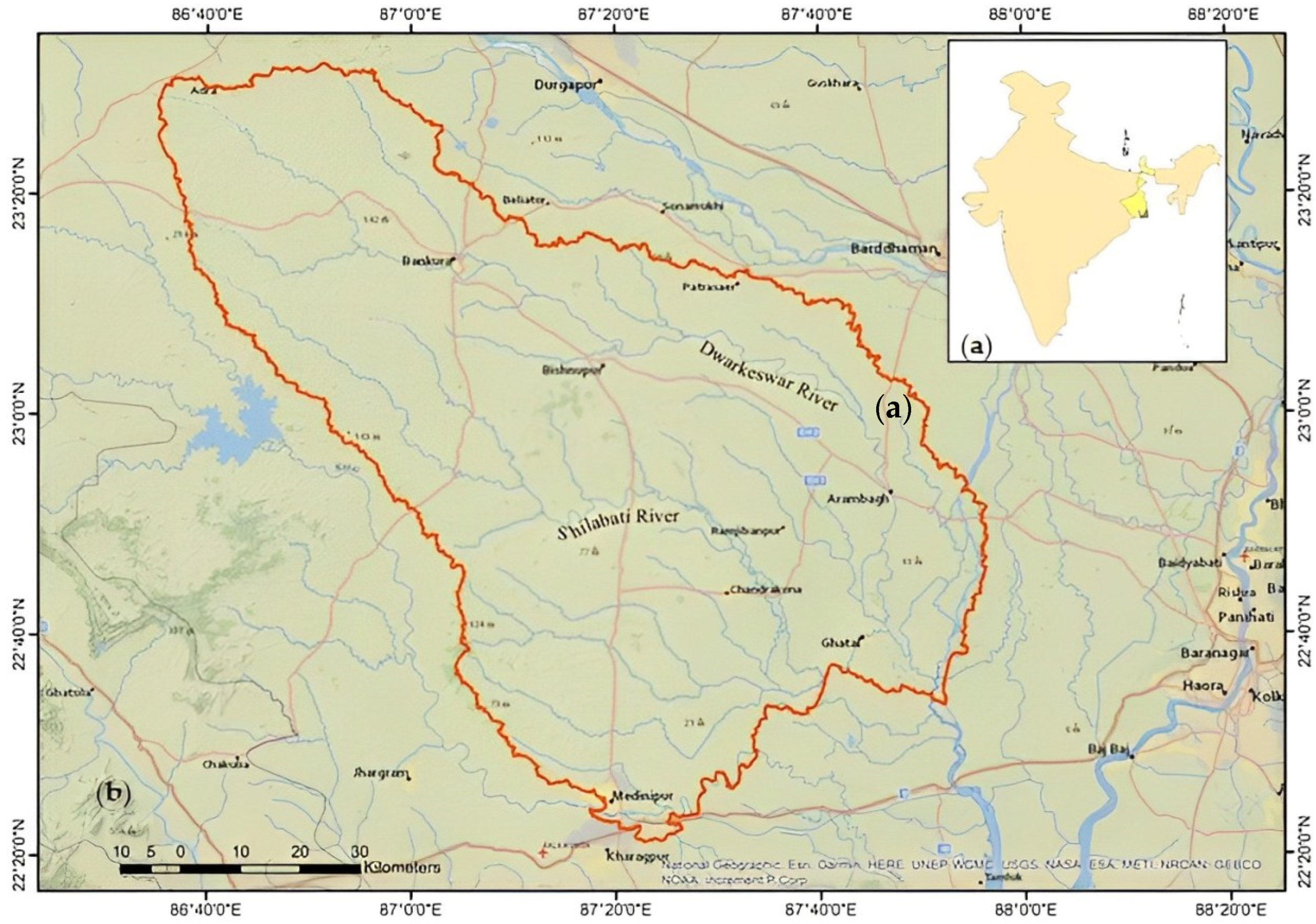
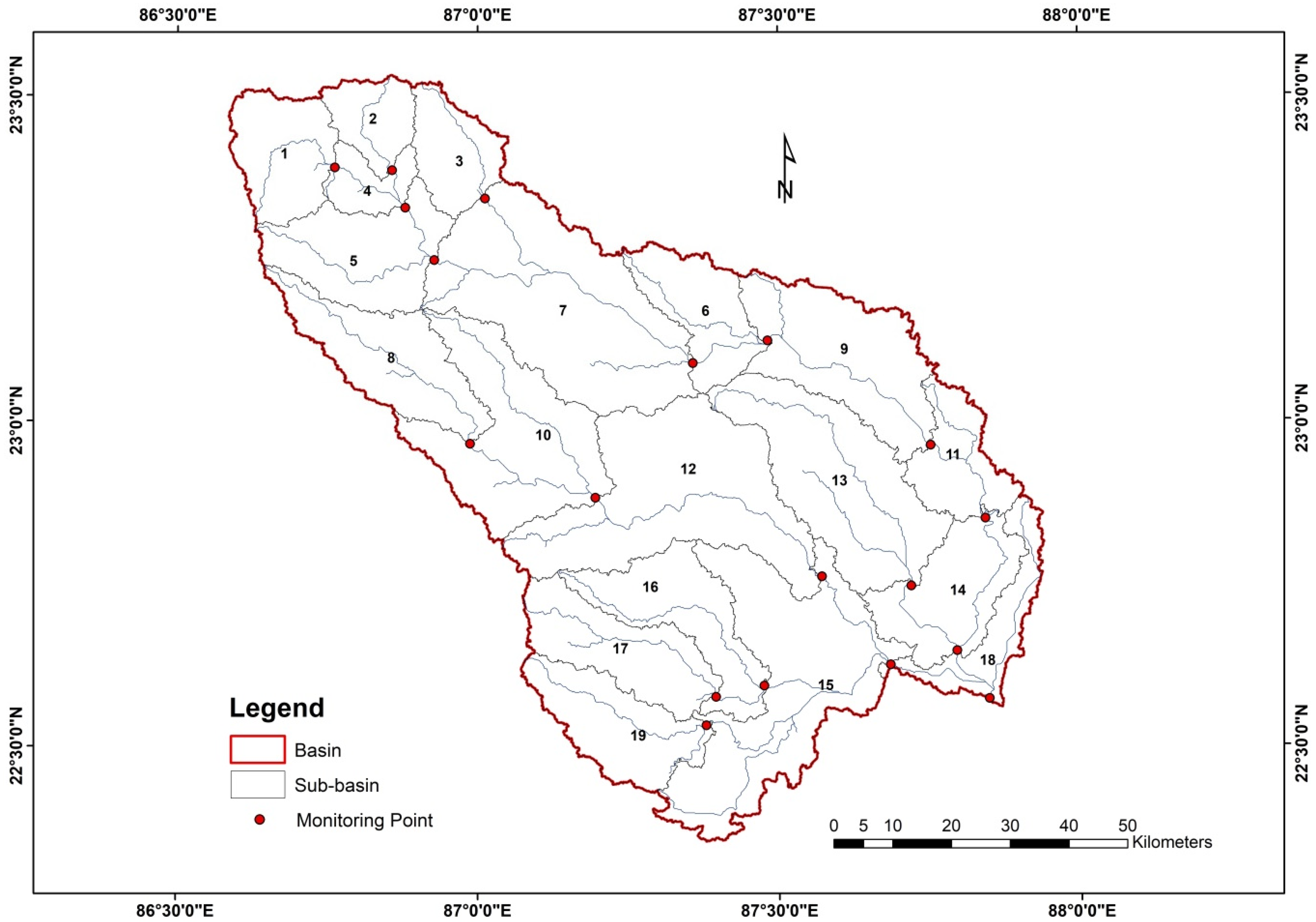
2. Study Area
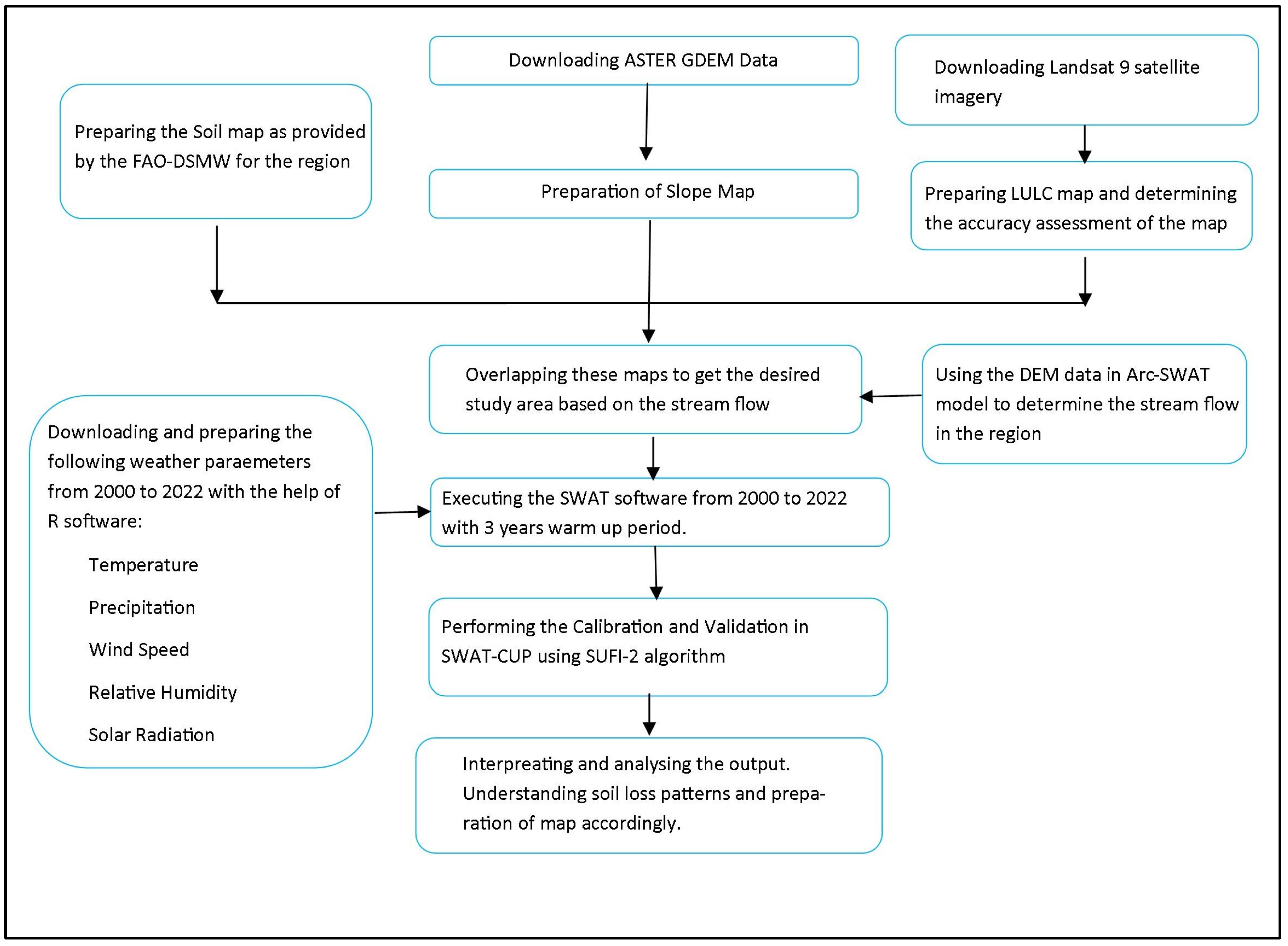
3. Methodology
3.1. Data Used
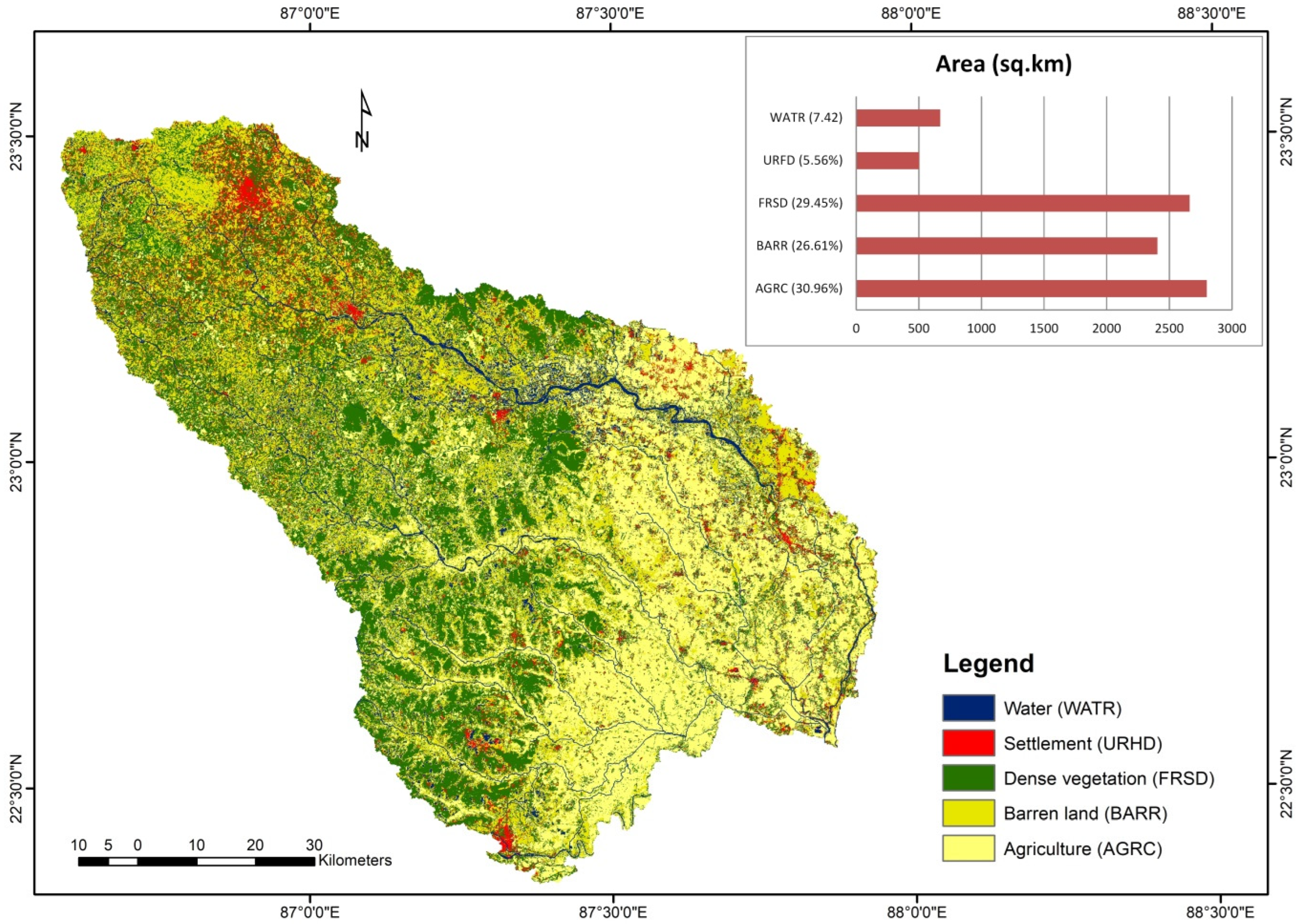
3.2. Preparation of Land Use and Land Cover (LULC) Maps
3.3. SWAT Setup
- SWo is the quantity of water on the first soil of the day in millimeters;
- t is the number of days;
- Rday represents the amount of precipitation on day i (mm);
- Qsurf represents the amount of surface runoff on a given day i (mm);
- Ea represents the amount of evapotranspiration on day i (mm);
- Wseep represents the amount of water that percolated into the vadose zone from the soil profile on day i (mm);
- Qgw represents the amount of return flow on day i (mm).
- Qsurf shows the surface runoff;
- qpeak represents the peak runoff rates;
- Ahru is the HRU’s area (in ha), KUSLE is the soil erodibility component;
- CUSLE shows the surface cover and crop management factor;
- PUSLE represents the conservation practice factor;
- LSUSLE is the topography factor; and
- CFRG means the coarse fragment factor.
3.4. Model Calibration and Validation
3.5. Assessment of Sediment Yield
4. Results and Discussion
4.1. Land Use Land Cover (LULC)
4.2. Soil Map
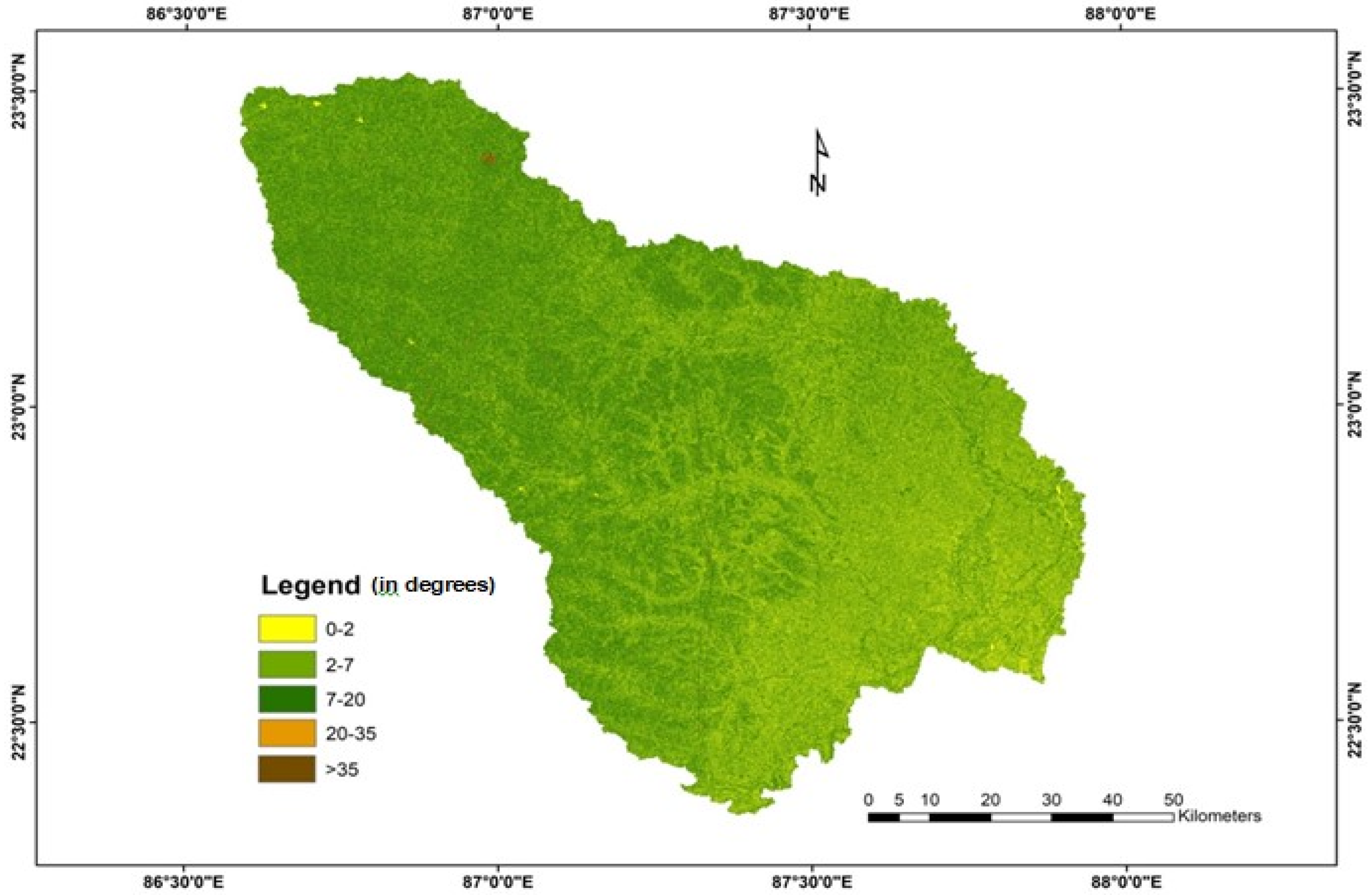
4.3. Slope Map
4.4. Watershed Delineation, and the Identification of Sub-Basins and HRUs
4.5. Sensitivity Analysis
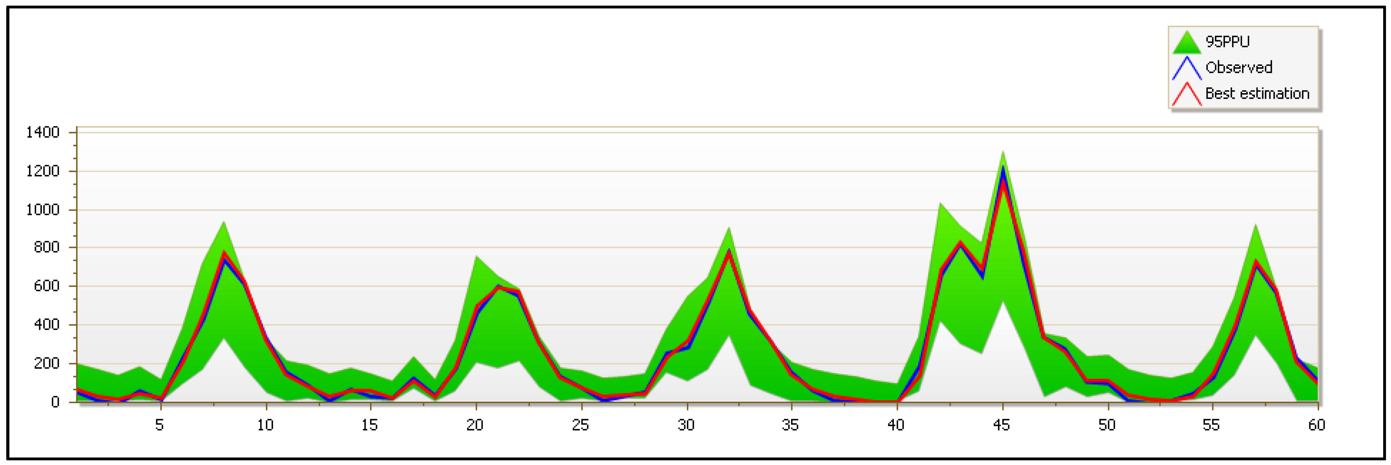
4.6. Model Calibration and Validation
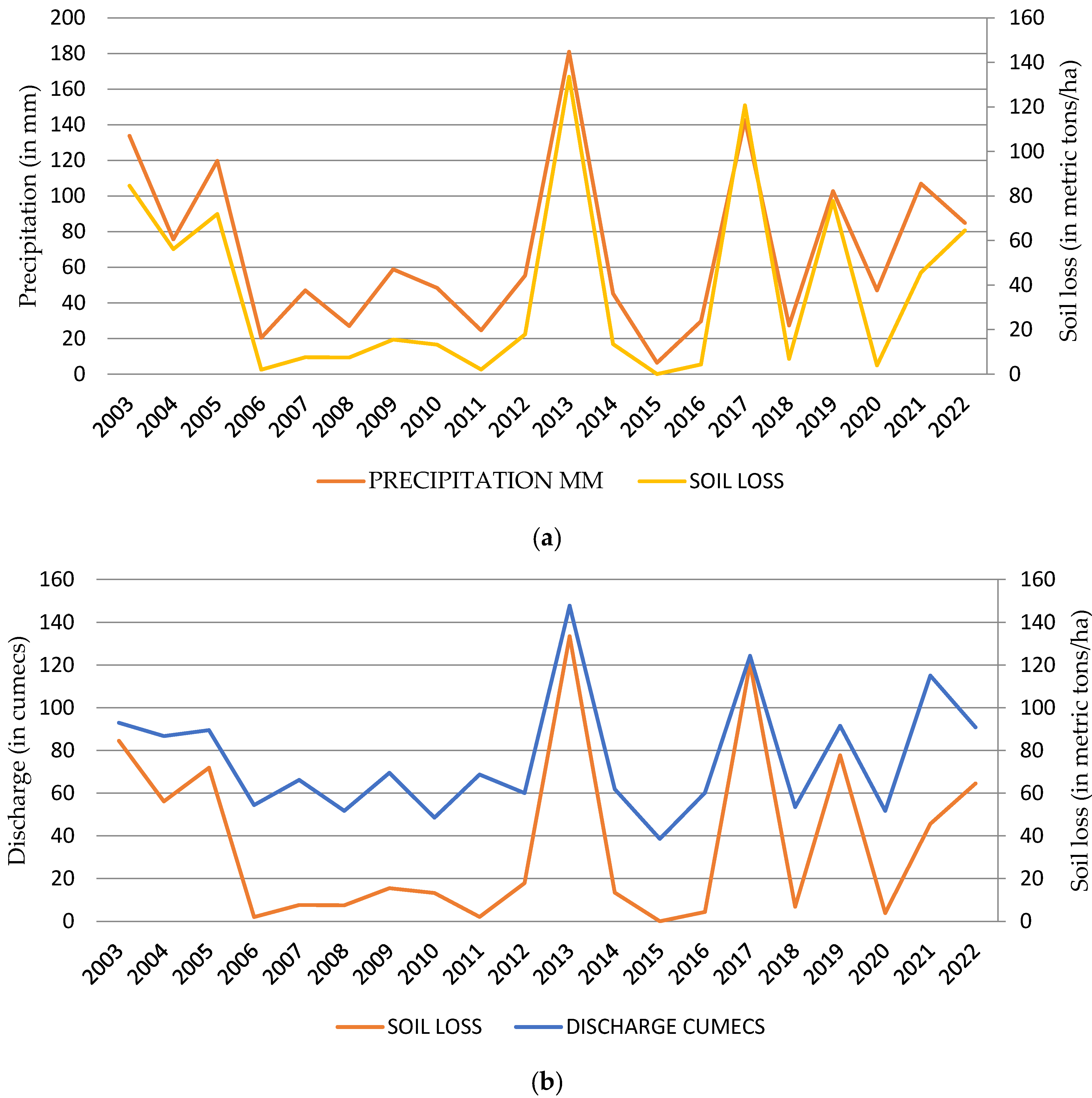
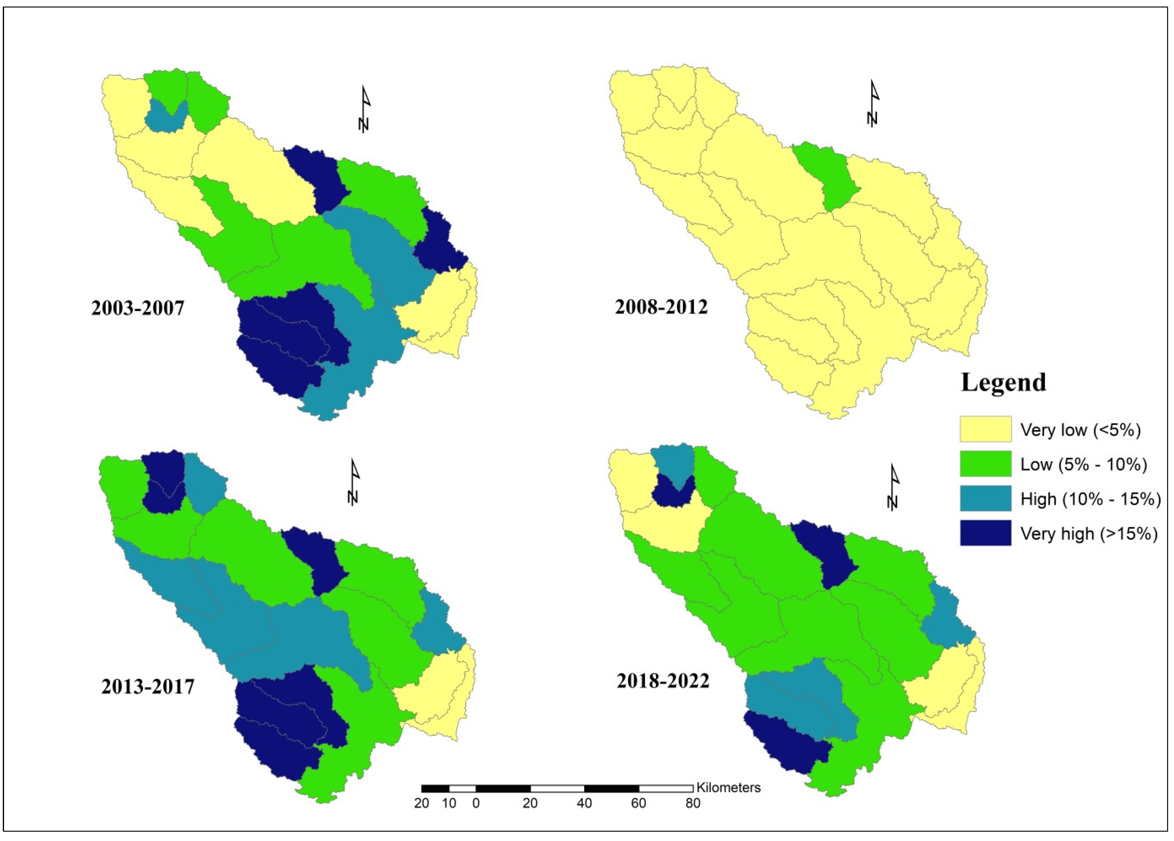
4.7. Loss of Sediment Yield
5. Conclusions
Author Contributions
Funding
Data Availability Statement
Conflicts of Interest
Appendix A

| Water | Forest | Agriculture | Barren | Urban | |
|---|---|---|---|---|---|
| Water | 9 | 0 | 0 | 1 | 0 |
| Forest | 0 | 39 | 9 | 0 | 0 |
| Agriculture | 0 | 3 | 40 | 1 | 0 |
| Barren | 0 | 0 | 2 | 41 | 0 |
| Urban | 0 | 1 | 0 | 0 | 10 |

| Sl. No. | HRU No. | Sub-Basin 1 | Area (sq. km) | % Watershed Area | % Sub-Basin Area |
|---|---|---|---|---|---|
| 1 | 1 | FRSD/Lf32-1b-3788/2-7 | 68.60 | 0.76 | 21.28 |
| 2 | 2 | FRSD/Lf32-1b-3788/7-20 | 61.67 | 0.68 | 19.13 |
| 3 | 3 | BARR/Lf32-1b-3788/7-20 | 82.65 | 0.91 | 25.64 |
| 4 | 4 | BARR/Lf32-1b-3788/2-7 | 109.42 | 1.21 | 33.95 |
| Sl. No. | HRU No. | Sub-Basin 2 | Area (sq. km) | % Watershed Area | % Sub-Basin Area |
| 1 | 5 | FRSD/Lf32-1b-3788/2-7 | 34.16 | 0.38 | 18.85 |
| 2 | 6 | FRSD/Lf32-1b-3788/7-20 | 33.83 | 0.37 | 18.67 |
| 3 | 7 | BARR/Lf32-1b-3788/2-7 | 64.11 | 0.71 | 35.37 |
| 4 | 8 | BARR/Lf32-1b-3788/7-20 | 49.13 | 0.54 | 27.11 |
| Sl. No. | HRU No. | Sub-Basin 3 | Area (sq. km) | % Watershed Area | % Sub-Basin Area |
| 1 | 9 | FRSD/Lf32-1b-3788/2-7 | 50.90 | 0.56 | 21.43 |
| 2 | 10 | FRSD/Lf32-1b-3788/7-20 | 52.29 | 0.58 | 22.01 |
| 3 | 11 | BARR/Lf32-1b-3788/2-7 | 42.21 | 0.47 | 17.77 |
| 4 | 12 | BARR/Lf32-1b-3788/7-20 | 34.95 | 0.39 | 14.71 |
| 5 | 13 | URHD/Lf32-1b-3788/7-20 | 26.58 | 0.29 | 11.19 |
| 6 | 14 | URHD/Lf32-1b-3788/2-7 | 30.63 | 0.34 | 12.89 |
| Sl. No. | HRU No. | Sub-Basin 4 | Area (sq. km) | % Watershed Area | % Sub-Basin Area |
| 1 | 15 | FRSD/Lf32-1b-3788/7-20 | 22.23 | 0.25 | 16.97 |
| 2 | 16 | FRSD/Lf32-1b-3788/2-7 | 20.37 | 0.23 | 15.55 |
| 3 | 17 | BARR/Lf32-1b-3788/2-7 | 34.57 | 0.38 | 26.39 |
| 4 | 18 | BARR/Lf32-1b-3788/7-20 | 29.84 | 0.33 | 22.78 |
| 5 | 19 | URHD/Lf32-1b-3788/2-7 | 12.51 | 0.14 | 9.55 |
| 6 | 20 | URHD/Lf32-1b-3788/7-20 | 11.49 | 0.13 | 8.77 |
| Sl. No. | HRU No. | Sub-Basin 5 | Area (sq. km) | % Watershed Area | % Sub-Basin Area |
| 1 | 21 | FRSD/Lf32-1b-3788/2-7 | 117.64 | 1.30 | 26.48 |
| 2 | 22 | FRSD/Lf32-1b-3788/7-20 | 126.52 | 1.40 | 28.48 |
| 3 | 23 | BARR/Lf32-1b-3788/7-20 | 93.27 | 1.03 | 21.00 |
| 4 | 24 | BARR/Lf32-1b-3788/2-7 | 106.77 | 1.18 | 24.04 |
| Sl. No. | HRU No. | Sub-Basin 6 | Area (sq. km) | % Watershed Area | % Sub-Basin Area |
| 1 | 25 | WATR/Be80-2a-3681/7-20 | 5.77 | 0.06 | 1.88 |
| 2 | 26 | WATR/Be80-2a-3681/2-7 | 15.48 | 0.17 | 5.04 |
| 3 | 27 | WATR/Be80-2a-3681/0-2 | 3.59 | 0.04 | 1.17 |
| 4 | 28 | WATR/Lf96-2ab-6668/7-20 | 7.62 | 0.08 | 2.48 |
| 5 | 29 | WATR/Lf96-2ab-6668/0-2 | 3.75 | 0.04 | 1.22 |
| 6 | 30 | WATR/Lf96-2ab-6668/2-7 | 18.51 | 0.20 | 6.02 |
| 7 | 31 | FRSD/Be80-2a-3681/7-20 | 18.39 | 0.20 | 5.98 |
| 8 | 32 | FRSD/Be80-2a-3681/2-7 | 18.15 | 0.20 | 5.91 |
| 9 | 33 | FRSD/Lf96-2ab-6668/7-20 | 38.44 | 0.43 | 12.51 |
| 10 | 34 | FRSD/Lf96-2ab-6668/2-7 | 40.31 | 0.45 | 13.12 |
| 11 | 35 | AGRC/Be80-2a-3681/2-7 | 14.71 | 0.16 | 4.79 |
| 12 | 36 | AGRC/Be80-2a-3681/0-2 | 3.06 | 0.03 | 1.00 |
| 13 | 37 | AGRC/Be80-2a-3681/7-20 | 5.48 | 0.06 | 1.78 |
| 14 | 38 | AGRC/Lf96-2ab-6668/2-7 | 14.32 | 0.16 | 4.66 |
| 15 | 39 | AGRC/Lf96-2ab-6668/0-2 | 3.43 | 0.04 | 1.12 |
| 16 | 40 | AGRC/Lf96-2ab-6668/7-20 | 5.65 | 0.06 | 1.84 |
| 17 | 41 | BARR/Be80-2a-3681/2-7 | 11.56 | 0.13 | 3.76 |
| 18 | 42 | BARR/Be80-2a-3681/7-20 | 6.77 | 0.07 | 2.20 |
| 19 | 43 | BARR/Be80-2a-3681/0-2 | 2.17 | 0.02 | 0.71 |
| 20 | 44 | BARR/Lf96-2ab-6668/2-7 | 40.36 | 0.45 | 13.13 |
| 21 | 45 | BARR/Lf96-2ab-6668/0-2 | 7.39 | 0.08 | 2.41 |
| 22 | 46 | BARR/Lf96-2ab-6668/7-20 | 22.42 | 0.25 | 7.30 |
| Sl. No. | HRU No. | Sub-Basin 7 | Area (sq. km) | % Watershed Area | % Sub-Basin Area |
| 1 | 46 | FRSD/Lf10-2a-6665/7-20 | 34.00 | 0.38 | 3.32 |
| 2 | 47 | FRSD/Lf10-2a-6665/2-7 | 40.50 | 0.45 | 3.96 |
| 3 | 48 | FRSD/Lf32-1b-3788/7-20 | 152.98 | 1.69 | 14.94 |
| 4 | 49 | FRSD/Lf32-1b-3788/2-7 | 153.08 | 1.69 | 14.95 |
| 5 | 50 | FRSD/Lf96-2ab-6668/7-20 | 55.51 | 0.61 | 5.42 |
| 6 | 51 | FRSD/Lf96-2ab-6668/2-7 | 57.40 | 0.64 | 5.61 |
| 7 | 52 | BARR/Lf10-2a-6665/7-20 | 34.27 | 0.38 | 3.35 |
| 8 | 53 | BARR/Lf10-2a-6665/0-2 | 13.76 | 0.15 | 1.34 |
| 9 | 54 | BARR/Lf10-2a-6665/2-7 | 68.47 | 0.76 | 6.69 |
| 10 | 55 | BARR/Lf32-1b-3788/2-7 | 164.14 | 1.82 | 16.03 |
| 11 | 56 | BARR/Lf32-1b-3788/7-20 | 121.42 | 1.34 | 11.86 |
| 12 | 57 | BARR/Lf96-2ab-6668/2-7 | 79.11 | 0.88 | 7.73 |
| 13 | 58 | BARR/Lf96-2ab-6668/7-20 | 49.16 | 0.54 | 4.80 |
| Sl. No. | HRU No. | Sub-Basin 8 | Area (sq. km) | % Watershed Area | % Sub-Basin Area |
| 1 | 58 | FRSD/I-Ne-3729/2-7 | 58.14 | 0.64 | 13.10 |
| 2 | 59 | FRSD/I-Ne-3729/7-20 | 73.17 | 0.81 | 16.48 |
| 3 | 60 | FRSD/Lf32-1b-3788/7-20 | 59.82 | 0.66 | 13.47 |
| 4 | 61 | FRSD/Lf32-1b-3788/2-7 | 50.10 | 0.55 | 11.28 |
| 5 | 62 | BARR/I-Ne-3729/2-7 | 44.07 | 0.49 | 9.93 |
| 6 | 63 | BARR/I-Ne-3729/7-20 | 41.94 | 0.46 | 9.45 |
| 7 | 64 | BARR/Lf32-1b-3788/7-20 | 52.08 | 0.58 | 11.73 |
| 8 | 65 | BARR/Lf32-1b-3788/2-7 | 64.63 | 0.72 | 14.56 |
| Sl. No. | HRU No. | Sub-Basin 9 | Area (sq. km) | % Watershed Area | % Sub-Basin Area |
| 1 | 66 | WATR/Be80-2a-3681/0-2 | 80.85 | 0.14 | 2.08 |
| 2 | 67 | WATR/Be80-2a-3681/7-20 | 132.91 | 0.18 | 2.81 |
| 3 | 68 | WATR/Be80-2a-3681/2-7 | 375.24 | 0.58 | 8.89 |
| 4 | 69 | FRSD/Be80-2a-3681/0-2 | 12.25 | 0.09 | 1.45 |
| 5 | 70 | FRSD/Be80-2a-3681/7-20 | 16.58 | 0.26 | 4.01 |
| 6 | 71 | FRSD/Be80-2a-3681/2-7 | 52.35 | 0.51 | 7.76 |
| 7 | 72 | AGRC/Be80-2a-3681/2-7 | 8.55 | 2.16 | 33.20 |
| 8 | 73 | AGRC/Be80-2a-3681/0-2 | 23.63 | 0.47 | 7.29 |
| 9 | 74 | AGRC/Be80-2a-3681/7-20 | 45.73 | 0.69 | 10.57 |
| 10 | 75 | BARR/Be80-2a-3681/7-20 | 195.56 | 0.34 | 5.17 |
| 11 | 76 | BARR/Be80-2a-3681/2-7 | 42.93 | 0.90 | 13.86 |
| 12 | 77 | BARR/Be80-2a-3681/0-2 | 62.26 | 0.19 | 2.91 |
| Sl. No. | HRU No. | Sub-Basin 10 | Area (sq. km) | % Watershed Area | % Sub-Basin Area |
| 1 | 77 | FRSD/Lf32-1b-3788/7-20 | 73.59 | 0.81 | 10.69 |
| 2 | 78 | FRSD/Lf32-1b-3788/2-7 | 64.14 | 0.71 | 9.32 |
| 3 | 79 | FRSD/Lf96-2ab-6668/7-20 | 92.82 | 1.03 | 13.48 |
| 4 | 80 | FRSD/Lf96-2ab-6668/2-7 | 88.67 | 0.98 | 12.88 |
| 5 | 81 | AGRC/Lf32-1b-3788/2-7 | 23.31 | 0.26 | 3.39 |
| 6 | 82 | AGRC/Lf32-1b-3788/7-20 | 23.97 | 0.27 | 3.48 |
| 7 | 83 | AGRC/Lf96-2ab-6668/7-20 | 30.72 | 0.34 | 4.46 |
| 8 | 84 | AGRC/Lf96-2ab-6668/2-7 | 49.55 | 0.55 | 7.20 |
| 9 | 85 | AGRC/Lf96-2ab-6668/0-2 | 9.50 | 0.11 | 1.38 |
| 10 | 86 | BARR/Lf32-1b-3788/2-7 | 60.56 | 0.67 | 8.80 |
| 11 | 87 | BARR/Lf32-1b-3788/7-20 | 46.31 | 0.51 | 6.73 |
| 12 | 88 | BARR/Lf96-2ab-6668/2-7 | 68.10 | 0.75 | 9.89 |
| 13 | 89 | BARR/Lf96-2ab-6668/7-20 | 44.50 | 0.49 | 6.46 |
| 14 | 90 | BARR/Lf96-2ab-6668/0-2 | 12.71 | 0.14 | 1.85 |
| Sl. No. | HRU No. | Sub-Basin 11 | Area (sq. km) | % Watershed Area | % Sub-Basin Area |
| 1 | 91 | FRSD/Be80-2a-3681/0-2 | 6.24 | 0.07 | 2.36 |
| 2 | 92 | FRSD/Be80-2a-3681/7-20 | 9.28 | 0.10 | 3.51 |
| 3 | 93 | FRSD/Be80-2a-3681/2-7 | 27.76 | 0.31 | 10.50 |
| 4 | 94 | AGRC/Be80-2a-3681/0-2 | 26.22 | 0.29 | 9.92 |
| 5 | 95 | AGRC/Be80-2a-3681/2-7 | 85.84 | 0.95 | 32.46 |
| 6 | 96 | AGRC/Je71-2a-3758/0-2 | 2.55 | 0.03 | 0.97 |
| 7 | 97 | AGRC/Je71-2a-3758/7-20 | 1.67 | 0.02 | 0.63 |
| 8 | 98 | AGRC/Je71-2a-3758/2-7 | 8.59 | 0.10 | 3.25 |
| 9 | 99 | BARR/Be80-2a-3681/2-7 | 66.06 | 0.73 | 24.98 |
| 10 | 100 | BARR/Be80-2a-3681/0-2 | 16.77 | 0.19 | 6.34 |
| 11 | 101 | BARR/Be80-2a-3681/7-20 | 13.44 | 0.15 | 5.08 |
| Sl. No. | HRU No. | Sub-Basin 12 | Area (sq. km) | % Watershed Area | % Sub-Basin Area |
| 1 | 102 | FRSD/Be80-2a-3681/7-20 | 35.33 | 0.39 | 3.72 |
| 2 | 103 | FRSD/Be80-2a-3681/2-7 | 49.92 | 0.55 | 5.26 |
| 3 | 104 | FRSD/Lf96-2ab-6668/7-20 | 128.82 | 1.43 | 13.58 |
| 4 | 105 | FRSD/Lf96-2ab-6668/2-7 | 155.94 | 1.73 | 16.44 |
| 5 | 106 | AGRC/Be80-2a-3681/0-2 | 155.94 | 0.20 | 1.88 |
| 6 | 107 | AGRC/Be80-2a-3681/2-7 | 17.88 | 0.75 | 7.17 |
| 7 | 108 | AGRC/Be80-2a-3681/7-20 | 68.00 | 0.23 | 2.17 |
| 8 | 109 | AGRC/Lf10-2a-6665/2-7 | 25.03 | 0.28 | 2.64 |
| 9 | 110 | AGRC/Lf10-2a-6665/7-20 | 7.57 | 0.08 | 0.80 |
| 10 | 111 | AGRC/Lf10-2a-6665/0-2 | 6.85 | 0.08 | 0.72 |
| 11 | 112 | AGRC/Lf96-2ab-6668/7-20 | 39.27 | 0.43 | 4.14 |
| 12 | 113 | AGRC/Lf96-2ab-6668/0-2 | 22.25 | 0.25 | 2.35 |
| 13 | 114 | AGRC/Lf96-2ab-6668/2-7 | 98.24 | 1.09 | 10.36 |
| 14 | 115 | BARR/Be80-2a-3681/2-7 | 54.13 | 0.60 | 5.71 |
| 15 | 116 | BARR/Be80-2a-3681/0-2 | 13.31 | 0.15 | 1.40 |
| 16 | 117 | BARR/Be80-2a-3681/7-20 | 16.26 | 0.18 | 1.71 |
| 17 | 118 | BARR/Lf96-2ab-6668/2-7 | 116.67 | 1.29 | 12.30 |
| 18 | 119 | BARR/Lf96-2ab-6668/7-20 | 47.04 | 0.52 | 4.96 |
| 19 | 120 | BARR/Lf96-2ab-6668/0-2 | 25.33 | 0.28 | 2.67 |
| Sl. No. | HRU No. | Sub-Basin 13 | Area (sq. km) | % Watershed Area | % Sub-Basin Area |
| 1 | 121 | FRSD/Be80-2a-3681/7-20 | 28.20 | 0.31 | 3.91 |
| 2 | 122 | FRSD/Be80-2a-3681/0-2 | 12.79 | 0.14 | 1.77 |
| 3 | 123 | FRSD/Be80-2a-3681/2-7 | 60.74 | 0.67 | 8.42 |
| 4 | 124 | AGRC/Be80-2a-3681/0-2 | 81.77 | 0.90 | 11.33 |
| 5 | 125 | AGRC/Be80-2a-3681/7-20 | 45.08 | 0.50 | 6.25 |
| 6 | 126 | AGRC/Be80-2a-3681/2-7 | 280.02 | 3.10 | 38.79 |
| 7 | 127 | AGRC/Lf10-2a-6665/2-7 | 62.03 | 0.69 | 8.59 |
| 8 | 128 | AGRC/Lf10-2a-6665/7-20 | 15.03 | 0.10 | 2.08 |
| 9 | 129 | AGRC/Lf10-2a-6665/0-2 | 15.28 | 0.17 | 2.12 |
| 10 | 130 | BARR/Be80-2a-3681/7-20 | 15.54 | 0.17 | 2.15 |
| 11 | 131 | BARR/Be80-2a-3681/2-7 | 70.59 | 0.78 | 9.78 |
| 12 | 132 | BARR/Be80-2a-3681/0-2 | 18.64 | 0.21 | 2.58 |
| 13 | 133 | BARR/Lf10-2a-6665/0-2 | 2.25 | 0.02 | 0.31 |
| 14 | 134 | BARR/Lf10-2a-6665/2-7 | 10.36 | 0.11 | 1.44 |
| 15 | 135 | BARR/Lf10-2a-6665/7-20 | 3.50 | 0.04 | 0.48 |
| Sl. No. | HRU No. | Sub-Basin 14 | Area (sq. km) | % Watershed Area | % Sub-Basin Area |
| 1 | 136 | FRSD/Be80-2a-3681/0-2 | 8.07 | 0.09 | 2.04 |
| 2 | 137 | FRSD/Be80-2a-3681/2-7 | 31.69 | 0.35 | 8.01 |
| 3 | 138 | FRSD/Be80-2a-3681/7-20 | 7.27 | 0.08 | 1.84 |
| 4 | 139 | FRSD/Je71-2a-3758/7-20 | 3.29 | 0.04 | 0.83 |
| 5 | 140 | FRSD/Je71-2a-3758/2-7 | 17.26 | 0.19 | 4.36 |
| 6 | 141 | FRSD/Je71-2a-3758/0-2 | 4.69 | 0.05 | 1.19 |
| 7 | 142 | AGRC/Be80-2a-3681/2-7 | 149.66 | 1.66 | 37.84 |
| 8 | 143 | AGRC/Be80-2a-3681/0-2 | 56.87 | 0.63 | 14.38 |
| 9 | 144 | AGRC/Je71-2a-3758/2-7 | 83.64 | 0.93 | 21.14 |
| 10 | 145 | AGRC/Je71-2a-3758/0-2 | 33.11 | 0.37 | 8.37 |
| Sl. No. | HRU No. | Sub-Basin 15 | Area (sq. km) | % Watershed Area | % Sub-Basin Area |
| 1 | 146 | FRSD/Lf10-2a-6665/2-7 | 38.63 | 0.43 | 4.16 |
| 2 | 147 | FRSD/Lf10-2a-6665/0-2 | 7.62 | 0.08 | 0.82 |
| 3 | 148 | FRSD/Lf10-2a-6665/7-20 | 17.72 | 0.20 | 1.91 |
| 4 | 149 | FRSD/Lf96-2ab-6668/2-7 | 23.58 | 0.26 | 2.54 |
| 5 | 150 | FRSD/Lf96-2ab-6668/7-20 | 9.11 | 0.10 | 0.98 |
| 6 | 151 | FRSD/Lf96-2ab-6668/0-2 | 5.29 | 0.06 | 0.57 |
| 7 | 152 | FRSD/Lo49-2a-3808/7-20 | 7.27 | 0.08 | 0.78 |
| 8 | 153 | FRSD/Lo49-2a-3808/2-7 | 23.79 | 0.26 | 2.56 |
| 9 | 154 | FRSD/Lo49-2a-3808/0-2 | 5.43 | 0.06 | 0.58 |
| 10 | 155 | AGRC/Lf32-1b-3788/2-7 | 299.32 | 3.31 | 32.24 |
| 11 | 156 | AGRC/Lf10-2a-6665/0-2 | 96.13 | 1.06 | 10.35 |
| 12 | 157 | AGRC/Lo49-2a-3808/7-20 | 26.44 | 0.29 | 2.85 |
| 13 | 158 | AGRC/Lo49-2a-3808/0-2 | 56.22 | 0.62 | 6.06 |
| 14 | 159 | AGRC/Lo49-2a-3808/2-7 | 174.05 | 1.93 | 18.75 |
| 15 | 160 | BARR/Lf10-2a-6665/7-20 | 8.06 | 0.09 | 0.87 |
| 16 | 161 | BARR/Lf10-2a-6665/2-7 | 39.65 | 0.44 | 4.27 |
| 17 | 162 | BARR/Lf10-2a-6665/0-2 | 11.16 | 0.12 | 1.20 |
| 18 | 163 | BARR/Lf96-2ab-6668/2-7 | 33.52 | 0.37 | 3.61 |
| 19 | 164 | ARR/Lf96-2ab-6668/7-20 | 7.16 | 0.08 | 0.77 |
| 20 | 165 | BARR/Lf96-2ab-6668/0-2 | 9.26 | 0.10 | 1.00 |
| 21 | 166 | BARR/Lo49-2a-3808/7-20 | 3.40 | 0.04 | 0.37 |
| 22 | 167 | BARR/Lo49-2a-3808/0-2 | 6.34 | 0.07 | 0.68 |
| 23 | 168 | BARR/Lo49-2a-3808/2-7 | 19.34 | 0.21 | 2.08 |
| Sl. No. | HRU No. | Sub-Basin 16 | Area (sq. km) | % Watershed Area | % Sub-Basin Area |
| 1 | 169 | FRSD/Lf10-2a-6665/0-2 | 3.50 | 0.04 | 0.86 |
| 2 | 170 | FRSD/Lf10-2a-6665/2-7 | 17.76 | 0.20 | 4.39 |
| 3 | 171 | FRSD/Lf10-2a-6665/7-20 | 7.15 | 0.08 | 1.77 |
| 4 | 172 | FRSD/Lf96-2ab-6668/7-20 | 49.01 | 0.54 | 12.11 |
| 5 | 173 | FRSD/Lf96-2ab-6668/2-7 | 73.83 | 0.82 | 18.25 |
| 6 | 174 | AGRC/Lf10-2a-6665/2-7 | 65.61 | 0.73 | 16.21 |
| 7 | 175 | AGRC/Lf10-2a-6665/0-2 | 22.59 | 0.25 | 5.58 |
| 8 | 176 | AGRC/Lf96-2ab-6668/2-7 | 45.95 | 0.51 | 11.35 |
| 9 | 177 | AGRC/Lf96-2ab-6668/0-2 | 11.50 | 0.13 | 2.84 |
| 10 | 178 | AGRC/Lf96-2ab-6668/7-20 | 13.74 | 0.15 | 3.40 |
| 11 | 179 | BARR/Lf10-2a-6665/0-2 | 6.16 | 0.07 | 1.52 |
| 12 | 180 | BARR/Lf10-2a-6665/2-7 | 19.94 | 0.22 | 4.93 |
| 13 | 181 | BARR/Lf10-2a-6665/7-20 | 3.12 | 0.03 | 0.77 |
| 14 | 182 | BARR/Lf96-2ab-6668/0-2 | 9.67 | 0.11 | 2.39 |
| 15 | 183 | BARR/Lf96-2ab-6668/7-20 | 13.99 | 0.15 | 3.46 |
| 16 | 184 | BARR/Lf96-2ab-6668/2-7 | 41.14 | 0.46 | 10.17 |
| Sl. No. | HRU No. | Sub-Basin 17 | Area (sq. km) | % Watershed Area | % Sub-Basin Area |
| 1 | 185 | FRSD/Lf10-2a-6665/2-7 | 16.32 | 0.18 | 4.14 |
| 2 | 186 | FRSD/Lf10-2a-6665/7-20 | 11.41 | 0.13 | 2.89 |
| 3 | 187 | FRSD/Lf96-2ab-6668/2-7 | 92.63 | 1.02 | 23.49 |
| 4 | 188 | FRSD/Lf96-2ab-6668/7-20 | 66.11 | 0.73 | 16.76 |
| 5 | 189 | AGRC/Lf10-2a-6665/2-7 | 15.65 | 0.17 | 3.97 |
| 6 | 190 | AGRC/Lf10-2a-6665/0-2 | 4.46 | 0.05 | 1.13 |
| 7 | 191 | AGRC/Lf10-2a-6665/7-20 | 4.86 | 0.05 | 1.23 |
| 8 | 192 | AGRC/Lf96-2ab-6668/2-7 | 48.87 | 0.54 | 12.39 |
| 9 | 193 | AGRC/Lf96-2ab-6668/7-20 | 18.99 | 0.21 | 4.82 |
| 10 | 194 | AGRC/Lf96-2ab-6668/0-2 | 11.11 | 0.12 | 2.82 |
| 11 | 195 | BARR/Lf10-2a-6665/0-2 | 1.80 | 0.02 | 0.46 |
| 12 | 196 | BARR/Lf10-2a-6665/2-7 | 7.66 | 0.08 | 1.94 |
| 13 | 197 | BARR/Lf10-2a-6665/7-20 | 3.02 | 0.03 | 0.77 |
| 14 | 198 | BARR/Lf96-2ab-6668/2-7 | 55.33 | 0.61 | 14.03 |
| 15 | 199 | BARR/Lf96-2ab-6668/0-2 | 11.47 | 0.13 | 2.91 |
| 16 | 200 | BARR/Lf96-2ab-6668/7-20 | 24.71 | 0.27 | 6.27 |
| Sl. No. | HRU No. | Sub-Basin 18 | Area (sq. km) | % Watershed Area | % Sub-Basin Area |
| 1 | 201 | FRSD/Be80-2a-3681/7-20 | 1.47 | 0.02 | 0.62 |
| 2 | 202 | FRSD/Be80-2a-3681/2-7 | 8.94 | 0.10 | 3.78 |
| 3 | 203 | FRSD/Be80-2a-3681/0-2 | 2.67 | 0.03 | 1.13 |
| 4 | 204 | FRSD/Je71-2a-3758/7-20 | 5.78 | 0.06 | 2.44 |
| 5 | 205 | FRSD/Je71-2a-3758/0-2 | 6.22 | 0.07 | 2.63 |
| 6 | 206 | FRSD/Je71-2a-3758/2-7 | 22.66 | 0.25 | 9.58 |
| 7 | 207 | AGRC/Be80-2a-3681/0-2 | 12.58 | 0.14 | 5.31 |
| 8 | 208 | AGRC/Be80-2a-3681/2-7 | 27.01 | 0.30 | 11.41 |
| 9 | 209 | AGRC/Je71-2a-3758/0-2 | 43.51 | 0.48 | 18.38 |
| 10 | 210 | AGRC/Je71-2a-3758/2-7 | 105.83 | 1.17 | 44.72 |
| Sl. No. | HRU No. | Sub-Basin 19 | Area (sq. km) | % Watershed Area | % Sub-Basin Area |
| 1 | 211 | FRSD/Lf10-2a-6665/2-7 | 15.59 | 0.17 | 4.15 |
| 2 | 212 | FRSD/Lf10-2a-6665/7-20 | 13.44 | 0.15 | 3.57 |
| 3 | 213 | FRSD/Lf96-2ab-6668/2-7 | 101.21 | 1.12 | 26.91 |
| 4 | 214 | FRSD/Lf96-2ab-6668/7-20 | 63.59 | 0.70 | 16.91 |
| 5 | 215 | AGRC/Lf10-2a-6665/2-7 | 4.02 | 0.04 | 1.07 |
| 6 | 216 | AGRC/Lf10-2a-6665/7-20 | 2.78 | 0.03 | 0.74 |
| 7 | 217 | AGRC/Lf96-2ab-6668/2-7 | 38.23 | 0.42 | 10.17 |
| 8 | 218 | AGRC/Lf96-2ab-6668/7-20 | 13.52 | 0.15 | 3.59 |
| 9 | 219 | AGRC/Lf96-2ab-6668/0-2 | 8.58 | 0.09 | 2.28 |
| 10 | 220 | BARR/Lf10-2a-6665/7-20 | 4.77 | 0.05 | 1.27 |
| 11 | 221 | BARR/Lf10-2a-6665/2-7 | 7.35 | 0.08 | 1.96 |
| 12 | 222 | BARR/Lf96-2ab-6668/0-2 | 13.69 | 0.15 | 3.64 |
| 13 | 223 | BARR/Lf96-2ab-6668/2-7 | 63.00 | 0.70 | 16.75 |
| 14 | 224 | BARR/Lf96-2ab-6668/7-20 | 26.28 | 0.29 | 6.99 |
| YEAR | 2003 | 2004 | 2005 | 2006 | 2007 | 2008 | 2009 | 2010 | 2011 | 2012 | 2013 | 2014 | 2015 | 2016 | 2017 | 2018 | 2019 | 2020 | 2021 | 2022 |
|---|---|---|---|---|---|---|---|---|---|---|---|---|---|---|---|---|---|---|---|---|
| Sub-Basin 1 | ||||||||||||||||||||
| PRECIPITATION (in mm) | 119.65 | 55.85 | 89.50 | 16.85 | 28.10 | 14.15 | 56.20 | 38.20 | 26.30 | 53.65 | 171.70 | 46.90 | 5.60 | 18.55 | 138.95 | 20.65 | 86.35 | 43.65 | 106.80 | 90.50 |
| DISCHARGE (in cumecs) | 14.02 | 11.88 | 10.99 | 7.97 | 9.17 | 6.87 | 10.09 | 5.84 | 10.45 | 9.63 | 22.64 | 9.63 | 5.33 | 9.09 | 19.61 | 7.68 | 13.22 | 7.98 | 17.45 | 14.82 |
| SOIL LOSS (metric tons/ha) | 21.45 | 13.90 | 26.68 | 0.38 | 1.30 | 0.49 | 5.69 | 1.70 | 1.50 | 6.59 | 57.80 | 11.66 | 0.05 | 0.36 | 32.39 | 1.41 | 20.53 | 2.26 | 19.58 | 22.41 |
| Sub-Basin 2 | ||||||||||||||||||||
| PRECIPITATION (in mm) | 119.65 | 55.85 | 89.50 | 16.85 | 28.10 | 14.15 | 56.20 | 38.20 | 26.30 | 53.65 | 171.70 | 46.90 | 5.60 | 18.55 | 138.95 | 20.65 | 86.35 | 43.65 | 106.80 | 90.50 |
| DISCHARGE (in cumecs) | 7.84 | 6.60 | 6.14 | 4.37 | 5.03 | 3.77 | 5.59 | 3.22 | 5.74 | 5.33 | 12.62 | 5.34 | 2.92 | 4.99 | 10.93 | 4.23 | 7.33 | 4.40 | 9.56 | 8.24 |
| SOIL LOSS (metric tons/ha) | 18.48 | 10.15 | 14.61 | 0.57 | 1.56 | 0.46 | 6.97 | 2.17 | 1.36 | 6.20 | 92.01 | 8.55 | 0.06 | 0.89 | 47.54 | 2.39 | 23.41 | 2.71 | 20.96 | 44.35 |
| Sub-Basin 3 | ||||||||||||||||||||
| PRECIPITATION (in mm) | 119.65 | 55.85 | 89.50 | 16.85 | 28.10 | 14.15 | 56.20 | 38.20 | 26.30 | 53.65 | 171.70 | 46.90 | 5.60 | 18.55 | 138.95 | 20.65 | 86.35 | 43.65 | 106.80 | 90.50 |
| DISCHARGE (in cumecs) | 10.34 | 8.82 | 8.10 | 6.03 | 6.92 | 5.19 | 7.52 | 4.23 | 7.92 | 7.18 | 16.70 | 7.16 | 4.04 | 6.84 | 14.55 | 5.76 | 9.75 | 6.00 | 12.59 | 10.95 |
| SOIL LOSS (metric tons/ha) | 30.68 | 14.47 | 43.02 | 0.47 | 0.47 | 0.52 | 7.58 | 2.43 | 0.65 | 6.77 | 56.94 | 15.62 | 0.06 | 0.48 | 58.70 | 1.59 | 24.11 | 2.16 | 24.07 | 50.25 |
| Sub-Basin 4 | ||||||||||||||||||||
| PRECIPITATION (in mm) | 119.65 | 55.85 | 89.50 | 16.85 | 28.10 | 14.15 | 56.20 | 38.20 | 26.30 | 53.65 | 171.70 | 46.90 | 5.60 | 18.55 | 138.95 | 20.65 | 86.35 | 43.65 | 106.80 | 90.50 |
| DISCHARGE (in cumecs) | 27.40 | 23.09 | 21.46 | 15.33 | 17.64 | 13.22 | 19.58 | 11.19 | 20.16 | 18.67 | 44.23 | 18.68 | 10.23 | 17.49 | 38.29 | 14.82 | 25.68 | 15.43 | 33.66 | 28.84 |
| SOIL LOSS (metric tons/ha) | 32.11 | 14.48 | 28.18 | 0.64 | 1.74 | 0.50 | 6.96 | 2.76 | 1.22 | 12.69 | 105.87 | 9.40 | 0.06 | 0.54 | 65.50 | 2.93 | 38.84 | 1.82 | 22.95 | 62.40 |
| Sub-Basin 5 | ||||||||||||||||||||
| PRECIPITATION (in mm) | 119.65 | 55.85 | 89.50 | 16.85 | 28.10 | 14.15 | 56.20 | 38.20 | 26.30 | 53.65 | 171.70 | 46.90 | 5.60 | 18.55 | 138.95 | 20.65 | 86.35 | 43.65 | 106.80 | 90.50 |
| DISCHARGE (in cumecs) | 47.43 | 40.55 | 37.20 | 27.77 | 31.88 | 23.90 | 34.56 | 20.15 | 36.27 | 33.05 | 76.45 | 32.98 | 18.64 | 31.59 | 66.52 | 26.57 | 45.02 | 27.53 | 59.35 | 50.42 |
| SOIL LOSS (metric tons/ha) | 32.11 | 7.40 | 11.43 | 0.60 | 1.30 | 0.57 | 5.80 | 1.42 | 1.39 | 8.57 | 59.21 | 10.00 | 0.03 | 0.70 | 79.57 | 1.41 | 26.60 | 2.95 | 26.24 | 16.57 |
| Sub-Basin 6 | ||||||||||||||||||||
| PRECIPITATION (in mm) | 121.65 | 69.15 | 119.65 | 19.00 | 43.60 | 26.20 | 56.50 | 42.90 | 22.60 | 57.05 | 170.90 | 42.75 | 5.45 | 20.20 | 144.05 | 20.05 | 86.60 | 39.95 | 106.60 | 93.45 |
| DISCHARGE (in cumecs) | 115.45 | 105.33 | 104.49 | 67.32 | 80.20 | 61.83 | 87.44 | 54.04 | 87.07 | 80.29 | 184.87 | 80.09 | 46.62 | 76.20 | 165.27 | 64.26 | 108.92 | 65.23 | 144.36 | 124.27 |
| SOIL LOSS (metric tons/ha) | 101.33 | 82.83 | 115.82 | 1.66 | 9.21 | 8.06 | 26.15 | 11.80 | 1.79 | 36.21 | 163.15 | 20.26 | 0.07 | 2.48 | 226.46 | 3.94 | 62.54 | 4.51 | 69.32 | 194.02 |
| Sub-Basin 7 | ||||||||||||||||||||
| PRECIPITATION (in mm) | 121.65 | 69.15 | 119.65 | 19.00 | 43.60 | 26.20 | 56.50 | 42.90 | 22.60 | 57.05 | 170.90 | 42.75 | 5.45 | 20.20 | 144.05 | 20.05 | 86.60 | 39.95 | 106.60 | 93.45 |
| DISCHARGE (in cumecs) | 102.17 | 92.35 | 90.86 | 59.59 | 70.68 | 54.28 | 76.99 | 47.26 | 77.11 | 71.06 | 163.77 | 70.86 | 41.08 | 67.47 | 145.86 | 56.80 | 96.44 | 57.86 | 127.94 | 109.81 |
| SOIL LOSS (metric tons/ha) | 75.31 | 56.37 | 93.85 | 1.32 | 10.26 | 8.74 | 17.82 | 7.20 | 2.10 | 27.71 | 132.57 | 15.58 | 0.09 | 2.19 | 201.30 | 4.56 | 93.54 | 4.64 | 55.57 | 107.80 |
| Sub-Basin 8 | ||||||||||||||||||||
| PRECIPITATION (in mm) | 119.65 | 55.85 | 89.50 | 16.85 | 28.10 | 14.15 | 56.20 | 38.20 | 26.30 | 53.65 | 171.70 | 46.90 | 5.60 | 18.55 | 138.95 | 20.65 | 86.35 | 43.65 | 106.80 | 90.50 |
| DISCHARGE (in cumecs) | 20.30 | 17.64 | 15.98 | 12.49 | 14.29 | 10.78 | 15.16 | 9.22 | 16.14 | 14.60 | 32.36 | 14.53 | 8.51 | 14.30 | 28.43 | 11.92 | 19.57 | 12.31 | 25.61 | 21.79 |
| SOIL LOSS (metric tons/ha) | 37.00 | 22.69 | 43.52 | 0.99 | 2.52 | 1.10 | 12.10 | 2.92 | 2.95 | 15.42 | 176.85 | 19.91 | 0.08 | 0.81 | 119.94 | 4.11 | 38.59 | 4.41 | 37.79 | 41.70 |
| Sub-Basin 9 | ||||||||||||||||||||
| PRECIPITATION (in mm) | 124.65 | 79.70 | 143.20 | 19.60 | 62.30 | 42.00 | 57.25 | 49.55 | 18.80 | 59.85 | 159.50 | 38.40 | 8.20 | 25.45 | 145.50 | 20.05 | 94.25 | 43.25 | 102.60 | 99.35 |
| DISCHARGE (in cumecs) | 138.63 | 128.68 | 132.89 | 78.74 | 98.03 | 76.77 | 105.80 | 66.72 | 102.52 | 95.22 | 221.10 | 93.88 | 55.80 | 89.55 | 199.64 | 75.87 | 131.53 | 77.60 | 173.95 | 149.43 |
| SOIL LOSS (metric tons/ha) | 78.74 | 58.96 | 56.99 | 1.10 | 10.18 | 9.18 | 12.59 | 8.93 | 0.50 | 14.58 | 60.53 | 6.03 | 0.05 | 2.05 | 108.37 | 1.28 | 62.15 | 1.67 | 34.64 | 57.50 |
| Sub-Basin 10 | ||||||||||||||||||||
| PRECIPITATION (in mm) | 143.85 | 82.75 | 126.55 | 22.00 | 47.40 | 25.30 | 60.65 | 53.10 | 26.40 | 54.90 | 195.95 | 48.60 | 5.60 | 35.85 | 141.35 | 33.95 | 110.00 | 50.45 | 106.60 | 80.20 |
| DISCHARGE (in cumecs) | 55.88 | 51.59 | 51.59 | 34.42 | 39.88 | 30.33 | 41.61 | 29.73 | 42.87 | 36.19 | 88.99 | 38.57 | 23.86 | 37.51 | 71.65 | 33.80 | 55.28 | 31.76 | 67.97 | 53.29 |
| SOIL LOSS (metric tons/ha) | 108.82 | 68.40 | 128.54 | 3.63 | 9.91 | 6.90 | 22.64 | 22.57 | 4.05 | 28.17 | 227.86 | 18.11 | 0.06 | 8.74 | 166.12 | 14.55 | 118.56 | 6.49 | 73.95 | 84.68 |
| Sub-Basin 11 | ||||||||||||||||||||
| PRECIPITATION (in mm) | 147.20 | 94.05 | 144.35 | 23.85 | 67.50 | 41.40 | 61.30 | 57.90 | 22.50 | 56.30 | 185.60 | 42.05 | 8.20 | 41.70 | 147.30 | 33.10 | 123.20 | 51.05 | 108.45 | 76.40 |
| DISCHARGE (in cumecs) | 151.30 | 140.41 | 146.43 | 84.55 | 106.29 | 83.54 | 114.15 | 73.49 | 109.79 | 101.53 | 240.35 | 100.22 | 59.99 | 96.10 | 214.80 | 82.08 | 144.36 | 83.31 | 188.30 | 158.81 |
| SOIL LOSS (metric tons/ha) | 108.79 | 67.33 | 66.81 | 2.26 | 11.45 | 11.34 | 13.86 | 23.61 | 1.86 | 14.92 | 101.32 | 5.86 | 0.03 | 5.77 | 74.37 | 6.65 | 110.42 | 2.70 | 36.50 | 24.77 |
| Sub-Basin 12 | ||||||||||||||||||||
| PRECIPITATION (in mm) | 143.85 | 82.75 | 126.55 | 22.00 | 47.40 | 25.30 | 60.65 | 53.10 | 26.40 | 54.90 | 195.95 | 48.60 | 5.60 | 35.85 | 141.35 | 33.95 | 110.00 | 50.45 | 106.60 | 80.20 |
| DISCHARGE (in cumecs) | 104.07 | 97.15 | 99.69 | 62.94 | 73.29 | 55.89 | 76.60 | 56.46 | 77.92 | 64.73 | 166.71 | 70.28 | 43.70 | 67.84 | 129.95 | 62.76 | 103.30 | 57.51 | 126.10 | 95.14 |
| SOIL LOSS (metric tons/ha) | 152.00 | 100.25 | 118.57 | 4.70 | 11.05 | 10.95 | 27.48 | 28.19 | 2.88 | 30.10 | 293.55 | 29.61 | 0.07 | 10.78 | 210.79 | 15.92 | 110.56 | 6.08 | 89.14 | 136.84 |
| Sub-Basin 13 | ||||||||||||||||||||
| PRECIPITATION (in mm) | 147.20 | 94.05 | 144.35 | 23.85 | 67.50 | 41.40 | 61.30 | 57.90 | 22.50 | 56.30 | 185.60 | 42.05 | 8.20 | 41.70 | 147.30 | 33.10 | 123.20 | 51.05 | 108.45 | 76.40 |
| DISCHARGE (in cumecs) | 36.04 | 34.80 | 38.85 | 19.32 | 26.10 | 21.67 | 25.65 | 21.46 | 23.69 | 19.53 | 55.32 | 20.35 | 14.78 | 21.18 | 44.05 | 20.15 | 38.17 | 18.58 | 43.83 | 28.57 |
| SOIL LOSS (metric tons/ha) | 193.70 | 112.40 | 86.04 | 4.88 | 19.18 | 25.52 | 24.70 | 32.02 | 3.22 | 28.38 | 143.31 | 10.28 | 0.08 | 10.58 | 166.01 | 8.98 | 169.70 | 5.01 | 72.23 | 63.50 |
| Sub-Basin 14 | ||||||||||||||||||||
| PRECIPITATION (in mm) | 147.20 | 94.05 | 144.35 | 23.85 | 67.50 | 41.40 | 61.30 | 57.90 | 22.50 | 56.30 | 185.60 | 42.05 | 8.20 | 41.70 | 147.30 | 33.10 | 123.20 | 51.05 | 108.45 | 76.40 |
| DISCHARGE (in cumecs) | 207.45 | 195.30 | 207.05 | 116.20 | 148.55 | 118.45 | 155.05 | 107.86 | 148.35 | 132.60 | 327.40 | 132.83 | 84.29 | 130.25 | 284.00 | 114.56 | 204.80 | 113.21 | 258.90 | 204.15 |
| SOIL LOSS (metric tons/ha) | 33.00 | 17.18 | 7.76 | 0.54 | 1.92 | 2.23 | 3.04 | 5.95 | 0.12 | 3.59 | 23.29 | 1.82 | 0.00 | 1.82 | 14.83 | 0.64 | 18.48 | 0.16 | 16.33 | 12.81 |
| Sub-Basin 15 | ||||||||||||||||||||
| PRECIPITATION (in mm) | 147.20 | 94.05 | 144.35 | 23.85 | 67.50 | 41.40 | 61.30 | 57.90 | 22.50 | 56.30 | 185.60 | 42.05 | 8.20 | 41.70 | 147.30 | 33.10 | 123.20 | 51.05 | 108.45 | 76.40 |
| DISCHARGE (in cumecs) | 213.40 | 203.75 | 213.40 | 130.14 | 155.45 | 121.36 | 159.35 | 123.49 | 159.65 | 130.50 | 338.00 | 142.13 | 93.38 | 140.00 | 264.50 | 130.49 | 217.45 | 118.80 | 260.60 | 190.10 |
| SOIL LOSS (metric tons/ha) | 194.01 | 134.31 | 167.00 | 4.32 | 23.17 | 30.37 | 27.56 | 38.36 | 5.20 | 28.43 | 206.37 | 12.51 | 0.16 | 10.96 | 197.02 | 18.87 | 170.22 | 7.59 | 75.80 | 79.82 |
| Sub-Basin 16 | ||||||||||||||||||||
| PRECIPITATION (in mm) | 143.85 | 82.75 | 126.55 | 22.00 | 47.40 | 25.30 | 60.65 | 53.10 | 26.40 | 54.90 | 195.95 | 48.60 | 5.60 | 35.85 | 141.35 | 33.95 | 110.00 | 50.45 | 106.60 | 80.20 |
| DISCHARGE (in cumecs) | 41.73 | 40.30 | 42.03 | 26.60 | 30.86 | 23.66 | 31.62 | 24.65 | 32.39 | 25.94 | 66.83 | 28.94 | 18.85 | 28.11 | 51.10 | 26.52 | 42.45 | 23.59 | 50.94 | 37.48 |
| SOIL LOSS (metric tons/ha) | 110.15 | 81.80 | 106.12 | 2.41 | 8.50 | 6.44 | 21.13 | 14.45 | 2.47 | 19.01 | 199.58 | 14.16 | 0.05 | 6.44 | 155.15 | 10.67 | 105.64 | 6.46 | 55.21 | 70.66 |
| Sub-Basin 17 | ||||||||||||||||||||
| PRECIPITATION (in mm) | 143.85 | 82.75 | 126.55 | 22.00 | 47.40 | 25.30 | 60.65 | 53.10 | 26.40 | 54.90 | 195.95 | 48.60 | 5.60 | 35.85 | 141.35 | 33.95 | 110.00 | 50.45 | 106.60 | 80.20 |
| DISCHARGE (in cumecs) | 20.61 | 19.88 | 20.73 | 13.11 | 15.22 | 11.65 | 15.59 | 12.15 | 15.95 | 12.79 | 32.95 | 14.24 | 9.25 | 13.86 | 25.20 | 13.03 | 20.92 | 11.60 | 25.11 | 18.48 |
| SOIL LOSS (metric tons/ha) | 121.65 | 84.42 | 107.23 | 3.18 | 8.46 | 7.52 | 24.13 | 20.23 | 2.55 | 22.70 | 229.15 | 21.89 | 0.07 | 8.65 | 212.07 | 13.33 | 122.77 | 5.17 | 64.16 | 70.23 |
| Sub-Basin 18 | ||||||||||||||||||||
| PRECIPITATION (in mm) | 147.20 | 94.05 | 144.35 | 23.85 | 67.50 | 41.40 | 61.30 | 57.90 | 22.50 | 56.30 | 185.60 | 42.05 | 8.20 | 41.70 | 147.30 | 33.10 | 123.20 | 51.05 | 108.45 | 76.40 |
| DISCHARGE (in cumecs) | 432.85 | 411.40 | 433.60 | 254.35 | 314.45 | 248.15 | 323.90 | 239.40 | 317.45 | 270.25 | 684.60 | 282.60 | 183.75 | 278.50 | 563.85 | 252.80 | 435.95 | 239.05 | 536.20 | 404.50 |
| SOIL LOSS (metric tons/ha) | 23.68 | 22.11 | 8.73 | 0.74 | 2.31 | 3.05 | 3.73 | 4.75 | 0.18 | 3.98 | 22.12 | 1.23 | 0.00 | 1.55 | 19.29 | 0.30 | 17.98 | 0.18 | 11.35 | 9.78 |
| Sub-Basin 19 | ||||||||||||||||||||
| PRECIPITATION (in mm) | 143.85 | 82.75 | 126.55 | 22.00 | 47.40 | 25.30 | 60.65 | 53.10 | 26.40 | 54.90 | 195.95 | 48.60 | 5.60 | 35.85 | 141.35 | 33.95 | 110.00 | 50.45 | 106.60 | 80.20 |
| DISCHARGE (in cumecs) | 19.64 | 18.84 | 19.68 | 12.34 | 14.34 | 10.97 | 14.74 | 11.47 | 14.98 | 12.07 | 31.32 | 13.43 | 8.66 | 13.06 | 23.92 | 12.25 | 19.81 | 10.91 | 23.77 | 17.50 |
| SOIL LOSS (metric tons/ha) | 133.63 | 97.78 | 135.16 | 3.76 | 9.94 | 8.22 | 24.48 | 19.78 | 2.96 | 25.83 | 186.41 | 23.21 | 0.04 | 7.30 | 138.36 | 15.75 | 142.06 | 6.63 | 61.03 | 76.40 |
References
- Arshad, M.; Martin, S. Identifying critical limits for soil quality indicators in agro-ecosystems. Agric. Ecosyst. Environ. 2002, 88, 153–160. [Google Scholar] [CrossRef]
- Nasir, M.J.; Ahmad, W.; Jun, C.; Iqbal, J.; Bateni, S.M. Soil erosion susceptibility assessment of Swat River sub-watersheds using the morphometry-based compound factor approach and GIS. Environ. Earth Sci. 2023, 82, 315. [Google Scholar] [CrossRef]
- Pimentel, D. Soil Erosion: A Food and Environmental Threat. Environ. Dev. Sustain. 2006, 8, 119–137. [Google Scholar] [CrossRef]
- Chalise, D.; Kumar, L.; Kristiansen, P. Land Degradation by Soil Erosion in Nepal: A Review. Soil Syst. 2019, 3, 12. [Google Scholar] [CrossRef]
- Pandey, S.; Kumar, P.; Zlatic, M.; Nautiyal, R.; Panwar, V.P. Recent advances in assessment of soil erosion vulnerability in a watershed. Int. Soil Water Conserv. Res. 2021, 9, 305–318. [Google Scholar] [CrossRef]
- Erenstein, O. The Economics of Soil Conservation in Developing Countries: The Case of Crop Residue Mulching; Wageningen University: Wageningen, The Netherlands, 1999. [Google Scholar]
- Tibebe, D.; Bewket, W. Surface runoff and soil erosion estimation using the SWAT model in the Keleta Watershed, Ethiopia. Land Degrad. Dev. 2010, 22, 551–564. [Google Scholar] [CrossRef]
- Mekonnen, Y.A.; Manderso, T.M. Land use/land cover change impact on streamflow using Arc-SWAT model, in case of Fetam watershed, Abbay Basin, Ethiopia. Appl. Water Sci. 2023, 13, 111. [Google Scholar] [CrossRef]
- Wischmeier, W.H.; Smith, D.D. Predicting Rainfall Erosion Losses: A Guide to Conservation Planning; Department of Agriculture, Science and Education Administration: Washington, DC, USA, 1978.
- Kaur, R.; Srinivasan, R.; Mishra, K.; Dutta, D.; Prasad, D.; Bansal, G. Assessment of a SWAT model for soil and water management in India. Land Use Water Resour. Res. 2003, 3, 1–7. [Google Scholar]
- Merritt, W.; Letcher, R.; Jakeman, A. A review of erosion and sediment transport models. Environ. Model. Softw. 2003, 18, 761–799. [Google Scholar] [CrossRef]
- Rawat, J.S.; Joshi, R.C.; Mesia, M. Estimation of erosivity index and soil loss under different land uses in the tropical foothills of Eastern Himalaya (India). Trop. Ecol. 2013, 54, 47–58. [Google Scholar]
- Bryan, R.B. Soil erodibility and processes of water erosion on hillslope. Geomorphology 2000, 32, 385–415. [Google Scholar] [CrossRef]
- Kouli, M.; Soupios, P.; Vallianatos, F. Soil erosion prediction using the Revised Universal Soil Loss Equation (RUSLE) in a GIS framework, Chania, Northwestern Crete, Greece. Environ. Geol. 2008, 57, 483–497. [Google Scholar] [CrossRef]
- Lal, R. Soil degradation by erosion. Land Degrad. Dev. 2001, 12, 519–539. [Google Scholar] [CrossRef]
- Morgan, R.P.C. Soil Erosion and Conservation, 3rd ed.; Blackwell: Malden, MA, USA, 2005. [Google Scholar]
- Panda, C.; Das, D.M.; Raul, S.K.; Sahoo, B.C. Sediment yield prediction and prioritization of sub-watersheds in the Upper Subarnarekha basin (India) using SWAT. Arab. J. Geosci. 2021, 14, 809. [Google Scholar] [CrossRef]
- Mosbahi, M.; Benabdallah, S.; Boussema, M.R. Assessment of soil erosion risk using SWAT model. Arab. J. Geosci. 2012, 6, 4011–4019. [Google Scholar] [CrossRef]
- Phuong, T.T.; Shrestha, R.P.; Chuong, H.V. Simulation of Soil Erosion Risk in the Upstream Area of Bo River Watershed. In Redefining Diversity & Dynamics of Natural Resources Management in Asia; Elsevier: Amsterdam, The Netherlands, 2017; Volume 3, pp. 87–99. [Google Scholar] [CrossRef]
- İrvem, A.; Topaloğlu, F.; Uygur, V. Estimating spatial distribution of soil loss over Seyhan River Basin in Turkey. J. Hydrol. 2007, 336, 30–37. [Google Scholar] [CrossRef]
- Terranova, O.; Antronico, L.; Coscarelli, R.; Iaquinta, P. Soil erosion risk scenarios in the Mediterranean environment using RUSLE and GIS: An application model for Calabria (southern Italy). Geomorphology 2009, 112, 228–245. [Google Scholar] [CrossRef]
- Demirci, A.; Karaburun, A. Estimation of soil erosion using RUSLE in a GIS framework: A case study in the Buyukcekmece Lake watershed, northwest Turkey. Environ. Earth Sci. 2011, 66, 903–913. [Google Scholar] [CrossRef]
- Ganasri, B.P.; Ramesh, H. Assessment of soil erosion by RUSLE model using remote sensing and GIS—A case study of Nethravathi Basin. Geosci. Front. 2016, 7, 953–961. [Google Scholar] [CrossRef]
- Pal, S.C.; Chakrabortty, R. Modeling of water induced surface soil erosion and the potential risk zone prediction in a sub-tropical watershed of Eastern India. Model. Earth Syst. Environ. 2018, 5, 369–393. [Google Scholar] [CrossRef]
- Williams, J.R. Sediment-Yield Prediction with Universal Equation Using Runoff Energy Factor. In Present and Prospective Technology for Predicting Sediment Yield and Sources; US Department of Agriculture, Agriculture Research Service: Washington, DC, USA, 1975; Volume 40. [Google Scholar]
- Beasley, D.B.; Huggins, L.F.; Monke, E.J. ANSWERS: A Model for Watershed Planning. Trans. ASAE 1980, 23, 0938–0944. [Google Scholar] [CrossRef]
- Young, R.A. AGNPS: A Non-Point-Source Pollution Model for Evaluating Agricultural Watersheds. J. Soil Water Conserv. 1989, 44, 168–173. [Google Scholar]
- Abbott, M.; Bathurst, J.; Cunge, J.; O’Connell, P.; Rasmussen, J. An introduction to the European Hydrological System—Systeme Hydrologique Europeen, “SHE”, 1: History and philosophy of a physically-based, distributed modelling system. J. Hydrol. 1986, 87, 45–59. [Google Scholar] [CrossRef]
- Ewen, J.; Parkin, G.; O’Connell, P.E. SHETRAN: Distributed River Basin Flow and Transport Modeling System. J. Hydrol. Eng. 2000, 5, 250–258. [Google Scholar] [CrossRef]
- Birkinshaw, S.J.; James, P.; Ewen, J. Graphical user interface for rapid set-up of SHETRAN physically-based river catchment model. Environ. Model. Softw. 2010, 25, 609–610. [Google Scholar] [CrossRef]
- Schulze, R.E. Hydrology and Agrohydrology: A Text to Accompany the ACRU 3.00 Agrohydrological Modelling System. In South Africa Water Research Commission Report, TT 95/69; Dept. of Agricultural Engineering, University of Natal: Pietermaritzburg, South Africa, 1995. [Google Scholar]
- Arnold, J.G.; Srinivasan, R.; Muttiah, R.S.; Williams, J.R. Large area hydrologic modeling and assessment Part I: Model development. JAWRA J. Am. Water Resour. Assoc. 1998, 34, 73–89. [Google Scholar] [CrossRef]
- Williams, J.R.; Arnold, J.G.; Kiniry, J.R.; Gassman, P.W.; Green, C.H. History of model development at Temple, Texas. Hydrol. Sci. J. 2008, 53, 948–960. [Google Scholar] [CrossRef]
- Gassman, P.W.; Reyes, M.R.; Green, C.H.; Arnold, J.G. The Soil and Water Assessment Tool: Historical Development, Applications, and Future Research Directions. Trans. ASABE 2007, 50, 1211–1250. [Google Scholar] [CrossRef]
- Arnold, J.G.; Moriasi, D.N.; Gassman, P.W.; Abbaspour, K.C.; White, M.J.; Srinivasan, R.; Santhi, C.; Harmel, R.D.; van Griensven, A.; Van Liew, M.W.; et al. SWAT: Model Use, Calibration, and Validation. Trans. ASABE 2012, 55, 1491–1508. [Google Scholar] [CrossRef]
- Gassman, P.W.; Sadeghi, A.M.; Srinivasan, R. Applications of the SWAT Model Special Section: Overview and Insights. J. Environ. Qual. 2014, 43, 1–8. [Google Scholar] [CrossRef]
- Devia, G.K.; Ganasri, B.; Dwarakish, G. A Review on Hydrological Models. Aquat. Procedia 2015, 4, 1001–1007. [Google Scholar] [CrossRef]
- Abbaspour, K.C.; Yang, J.; Maximov, I.; Siber, R.; Bogner, K.; Mieleitner, J.; Zobrist, J.; Srinivasan, R. Modelling hydrology and water quality in the pre-alpine/alpine Thur watershed using SWAT. J. Hydrol. 2007, 333, 413–430. [Google Scholar] [CrossRef]
- Malik, S.; Pal, S.C. Potential flood frequency analysis and susceptibility mapping using CMIP5 of MIROC5 and HEC-RAS model: A case study of lower Dwarkeswar River, Eastern India. SN Appl. Sci. 2021, 3, 31. [Google Scholar] [CrossRef]
- Inland River Ports. Inland Waterway Transport; Inland River Ports: St. Louis, MO, USA, 2016; pp. 141–157. [Google Scholar] [CrossRef]
- Shit, P.K.; Maiti, R. Rill Hydraulics—An Experimental Study on Gully Basin in Lateritic Upland of Paschim Medinipur, West Bengal, India. J. Geogr. Geol. 2012, 4, 1. [Google Scholar] [CrossRef]
- Bera, B.; Saha, S.; Bhattacharjee, S. Forest cover dynamics (1998 to 2019) and prediction of deforestation probability using binary logistic regression (BLR) model of Silabati watershed, India. Trees For. People 2020, 2, 100034. [Google Scholar] [CrossRef]
- Mahala, A. Processes and Status of Land Degradation in a Plateau Fringe Region of Tropical Environment. Environ. Process. 2017, 4, 663–682. [Google Scholar] [CrossRef]
- Nag, S.K.; Lahiri, A. Hydrochemical Characteristics of Groundwater for Domestic and Irrigation Purposes in Dwarakeswar Watershed Area, India. Am. J. Clim. Chang. 2012, 1, 217–230. [Google Scholar] [CrossRef]
- Saraf, A.K.; Choudhury, P.R.; Roy, B.; Sarma, B.; Vijay, S.; Choudhury, S. GIS based surface hydrological modelling in identification of groundwater recharge zones. Int. J. Remote. Sens. 2004, 25, 5759–5770. [Google Scholar] [CrossRef]
- Cervantes, J.; Garcia-Lamont, F.; Rodríguez-Mazahua, L.; Lopez, A. A comprehensive survey on support vector machine classification: Applications, challenges and trends. Neurocomputing 2019, 408, 189–215. [Google Scholar] [CrossRef]
- Halder, S.; Das, S.; Basu, S. Use of support vector machine and cellular automata methods to evaluate impact of irrigation project on LULC. Environ. Monit. Assess. 2022, 195, 3. [Google Scholar] [CrossRef] [PubMed]
- Zhang, Y. Support Vector Machine Classification Algorithm and Its Application. In Information Computing and Applications: Third International Conference, ICICA 2012, Chengde, China, 14–16 September 2012. Proceedings, Part II 3; Springer: Berlin/Heidelberg, Germany, 2012; pp. 179–186. [Google Scholar] [CrossRef]
- Krause, P.; Boyle, D.P.; Bäse, F. Comparison of different efficiency criteria for hydrological model assessment. Adv. Geosci. 2005, 5, 89–97. [Google Scholar] [CrossRef]
- Nash, J.E.; Sutcliffe, J.V. River flow forecasting through conceptual models part I—A discussion of principles. J. Hydrol. 1970, 10, 282–290. [Google Scholar] [CrossRef]
- Gupta, H.V.; Sorooshian, S.; Yapo, P.O. Status of Automatic Calibration for Hydrologic Models: Comparison with Multilevel Expert Calibration. J. Hydrol. Eng. 1999, 4, 135–143. [Google Scholar] [CrossRef]
- Das, B.; Jain, S.; Singh, S.; Thakur, P. Evaluation of multisite performance of SWAT model in the Gomti River Basin, India. Appl. Water Sci. 2019, 9, 134. [Google Scholar] [CrossRef]
- Moriasi, D.N.; Arnold, J.G.; van Liew, M.W.; Bingner, R.L.; Harmel, R.D.; Veith, T.L. Model evaluation guidelines for systematic quantification of accuracy in watershed simulations. Trans. ASABE 2007, 50, 885–900. [Google Scholar] [CrossRef]
- Abbaspour, K.C.; Rouholahnejad, E.; Vaghefi, S.; Srinivasan, R.; Yang, H.; Kløve, B. A continental-scale hydrology and water quality model for Europe: Calibration and uncertainty of a high-resolution large-scale SWAT model. J. Hydrol. 2015, 524, 733–752. [Google Scholar] [CrossRef]
- Abbaspour, K.C.; Johnson, C.A.; van Genuchten, M.T. Estimating Uncertain Flow and Transport Parameters Using a Sequential Uncertainty Fitting Procedure. Vadose Zone J. 2004, 3, 1340–1352. [Google Scholar] [CrossRef]
- Yang, J.; Reichert, P.; Abbaspour, K.C.; Xia, J.; Yang, H. Comparing uncertainty analysis techniques for a SWAT application to the Chaohe Basin in China. J. Hydrol. 2008, 358, 1–23. [Google Scholar] [CrossRef]
- Aown, A.; Kar, N.S. Lateritic Badland of Sinhati, Bankura, West Bengal: A Geomorphic Investigation. In Neo-Thinking on Ganges-Brahmaputra Basin Geomorphology; Springer: Berlin/Heidelberg, Germany, 2016; pp. 19–31. [Google Scholar] [CrossRef]
- Shit, P.K.; Bhunia, G.S.; Maiti, R. Farmers’ Perceptions of Soil Erosion and Management Strategies in South Bengal in India. Eur. J. Geogr. 2015, 6, 85–100. [Google Scholar]
- David, S.R.; Murphy, B.P.; Czuba, J.A.; Ahammad, M.; Belmont, P. USUAL Watershed Tools: A new geospatial toolkit for hydro-geomorphic delineation. Environ. Model. Softw. 2023, 159, 105576. [Google Scholar] [CrossRef]
- Narsimlu, B.; Gosain, A.K.; Chahar, B.R. Assessment of Future Climate Change Impacts on Water Resources of Upper Sind River Basin, India Using SWAT Model. Water Resour. Manag. 2013, 27, 3647–3662. [Google Scholar] [CrossRef]
- Narsimlu, B.; Gosain, A.K.; Chahar, B.R.; Singh, S.K.; Srivastava, P.K. SWAT Model Calibration and Uncertainty Analysis for Streamflow Prediction in the Kunwari River Basin, India, Using Sequential Uncertainty Fitting. Environ. Process. 2015, 2, 79–95. [Google Scholar] [CrossRef]
- Suryavanshi, S.; Pandey, A.; Chaube, U.C. Hydrological Simulation of the Betwa River Basin (India) Using the SWAT Model. Hydrol. Sci. J. 2017, 62, 960–978. [Google Scholar] [CrossRef]
- Khatun, S.; Sahana, M.; Jain, S.K.; Jain, N. Simulation of surface runoff using semi distributed hydrological model for a part of Satluj Basin: Parameterization and global sensitivity analysis using SWAT CUP. Model. Earth Syst. Environ. 2018, 4, 1111–1124. [Google Scholar] [CrossRef]
- James, L.D.; Burges, S.J. Selection, Calibration, and Testing of Hydrologic Models. In Hydrologic Modeling of Small Watersheds; Haan, C.T., Johnson, H.P., Brakensiek, D.L., Eds.; ASAE Monograph; ASAE: St. Joseph, MI, USA, 1982; pp. 437–472. [Google Scholar]
- Kværnø, S.H.; Stolte, J. Effects of soil physical data sources on discharge and soil loss simulated by the LISEM model. Catena 2012, 97, 137–149. [Google Scholar] [CrossRef]


| Sl. No. | Data | Description | Source |
|---|---|---|---|
| 1. | Digital Elevation Model (DEM) | 30 m × 30 m spatial resolution grid used to delineate the boundary of the watershed. | Advanced Spaceborne Thermal Emission and Reflection Global Radiometer (ASTER) data from the United States Geological Survey (USGS) |
| 2. | Landsat 9 | To understand how the soil has been used and the current landscape; prepared by supervised classification. Resolution: 30 m × 30 m | United States Geological Survey (USGS) |
| 3. | Soil Data | To understand the soil structure and geological structure of the watershed. Scale: 1:5,000,000 | Food and Agricultural Organization Digital Soil Map of the World (FAO-DSMW) |
| 4. | Weather | Precipitation, solar radiation, relative humidity, wind, and temperature for 30 gauge stations in and around the area from 2000 to 2022. Resolution: 0.5 × 0.625 | NASA Prediction of Worldwide Energy Resources (POWER) |
| Rank | Parameters | Description | Maximum Value | Minimum Value | Fitted Value |
|---|---|---|---|---|---|
| 1 | CN2 | Curve number II | 30 | 450 | 0.016 |
| 2 | GW_DELAY | Groundwater delay time | 0 | 1 | 53.100 |
| 3 | ALPHA_BF | Base flow alpha factor | 0 | 2 | 0.109 |
| 4 | GWQMN | Threshold depth of water in the shallow aquifer required for return flow | 0 | 2 | 0.138 |
| 5 | GW_REVAP | Groundwater “revap” coefficient | 0 | 500 | 0.110 |
| 6 | REVAPMN | Threshold depth of water in the shallow aquifer for “revap” to occur | −0.2 | 0.4 | 312.500 |
| 7 | SOL_AWC | Soil available water capacity | 0.8 | 1 | 0.192 |
| 8 | ESCO | Soil evaporation compensation factor | −0.8 | 0.8 | 0.942 |
| 9 | SOL_K | Saturated hydraulic conductivity | 0 | 1 | −0.254 |
| 10 | ALPHA_BNK | Base flow alpha factor for bank storage | 5 | 130 | 0.525 |
| 11 | CH_K2 | Effective hydraulic conductivity in the main channel | 0 | 1 | 30.875 |
| 12 | EPCO | Plant uptake compensation factor | 0 | 1 | 0.127 |
| 13 | HRU_SLP | Average slope steepness | 0 | 0.3 | 0.787 |
| 14 | CH_N2 | Manning’s “n” value for the main channel | 0.01 | 1 | 0.104 |
| 15 | OV_N | Manning’s “n” value for overland flow | −0.5 | 0.6 | 0.793 |
| 16 | SLSUBBSN | Average slope length | −0.5 | 0.6 | 20.220 |
| 17 | SOL_BD | Moist bulk density | 0.05 | 24 | −0.492 |
| 18 | SURLAG | Surface runoff lag time | 30 | 450 | 0.016 |
| Process | R2 | NSE | P-Factor | R-Factor | PBIAS |
|---|---|---|---|---|---|
| Calibration (2003–2017) | 0.95 | 0.97 | 0.77 | 0.89 | −0.6 |
| Validation (2018–2022) | 0.92 | 0.93 | 0.98 | 0.87 | −2.7 |
| Sub-Basin | Area (ha) | 2003–2007 | 2008–2012 | 2013–2017 | 2018–2022 | ||||
|---|---|---|---|---|---|---|---|---|---|
| Soil loss (metric tons/ha) | % soil loss | Soil loss (metric tons/ha) | % soil loss | Soil loss (metric tons/ha) | % soil loss | Soil loss (metric tons/ha) | % soil loss | ||
| 1 | 322.35 | 12.74 | 3.95 | 3.19 | 0.99 | 20.45 | 6.35 | 13.24 | 4.11 |
| 2 | 181.24 | 9.07 | 5.01 | 3.43 | 1.89 | 29.81 | 16.45 | 18.76 | 10.35 |
| 3 | 237.57 | 17.82 | 7.50 | 3.59 | 1.51 | 26.36 | 11.10 | 20.44 | 8.60 |
| 4 | 131.00 | 15.43 | 11.78 | 4.83 | 3.69 | 36.27 | 27.69 | 25.79 | 19.69 |
| 5 | 444.20 | 10.57 | 2.38 | 3.55 | 0.80 | 29.90 | 6.73 | 14.76 | 3.32 |
| 6 | 307.36 | 62.17 | 20.23 | 16.80 | 5.47 | 82.49 | 26.84 | 66.87 | 21.76 |
| 7 | 1023.80 | 47.42 | 4.63 | 12.71 | 1.24 | 70.35 | 6.87 | 53.22 | 5.20 |
| 8 | 443.94 | 21.34 | 4.81 | 6.90 | 1.55 | 63.52 | 14.31 | 25.32 | 5.70 |
| 9 | 589.00 | 41.19 | 6.99 | 9.15 | 1.55 | 35.40 | 6.01 | 31.45 | 5.34 |
| 10 | 688.45 | 63.86 | 9.28 | 16.86 | 2.45 | 84.18 | 12.23 | 59.65 | 8.66 |
| 11 | 264.43 | 51.33 | 19.41 | 13.12 | 4.96 | 37.47 | 14.17 | 36.21 | 13.69 |
| 12 | 948.48 | 77.32 | 8.15 | 19.92 | 2.10 | 108.96 | 11.49 | 71.71 | 7.56 |
| 13 | 721.82 | 83.24 | 11.53 | 22.77 | 3.15 | 66.05 | 9.15 | 63.88 | 8.85 |
| 14 | 395.55 | 12.08 | 3.05 | 2.99 | 0.76 | 8.35 | 2.11 | 9.69 | 2.45 |
| 15 | 928.48 | 104.56 | 11.26 | 25.98 | 2.80 | 85.40 | 9.20 | 70.46 | 7.59 |
| 16 | 404.65 | 61.80 | 15.27 | 12.70 | 3.14 | 75.07 | 18.55 | 49.73 | 12.29 |
| 17 | 394.41 | 64.99 | 16.48 | 15.43 | 3.91 | 94.37 | 23.93 | 55.13 | 13.98 |
| 18 | 236.67 | 11.51 | 4.86 | 3.14 | 1.33 | 8.84 | 3.73 | 7.92 | 3.35 |
| 19 | 376.03 | 76.06 | 20.23 | 16.26 | 4.32 | 71.06 | 18.90 | 60.38 | 16.06 |
Disclaimer/Publisher’s Note: The statements, opinions and data contained in all publications are solely those of the individual author(s) and contributor(s) and not of MDPI and/or the editor(s). MDPI and/or the editor(s) disclaim responsibility for any injury to people or property resulting from any ideas, methods, instructions or products referred to in the content. |
© 2024 by the authors. Licensee MDPI, Basel, Switzerland. This article is an open access article distributed under the terms and conditions of the Creative Commons Attribution (CC BY) license (https://creativecommons.org/licenses/by/4.0/).
Share and Cite
Mukherjee, A.; Kumari, M.; Mishra, V.N. Assessing Post-Monsoon Seasonal Soil Loss over Un-Gauged Stations of the Dwarkeswar and Shilabati Rivers, West Bengal, India. Earth 2024, 5, 45-71. https://doi.org/10.3390/earth5010003
Mukherjee A, Kumari M, Mishra VN. Assessing Post-Monsoon Seasonal Soil Loss over Un-Gauged Stations of the Dwarkeswar and Shilabati Rivers, West Bengal, India. Earth. 2024; 5(1):45-71. https://doi.org/10.3390/earth5010003
Chicago/Turabian StyleMukherjee, Ankita, Maya Kumari, and Varun Narayan Mishra. 2024. "Assessing Post-Monsoon Seasonal Soil Loss over Un-Gauged Stations of the Dwarkeswar and Shilabati Rivers, West Bengal, India" Earth 5, no. 1: 45-71. https://doi.org/10.3390/earth5010003
APA StyleMukherjee, A., Kumari, M., & Mishra, V. N. (2024). Assessing Post-Monsoon Seasonal Soil Loss over Un-Gauged Stations of the Dwarkeswar and Shilabati Rivers, West Bengal, India. Earth, 5(1), 45-71. https://doi.org/10.3390/earth5010003