Monitoring Gas Emissions in Agricultural Productions through Low-Cost Technologies: The POREM (Poultry-Manure-Based Bio-Activator for Better Soil Management through Bioremediation) Project Experience

Abstract

Agricultural production or rural activities can involve the emission of unpleasant gases, malodors, or most commonly, greenhouse gases. In any case, the control and monitoring of such emissions in rural, unattended, and remote locations represent an issue in need of addressing. In this article, the monitoring of gases produced by a poultry manure depot and performed by devices based on low-cost gas sensors in the context of the POREM (poultry-manure-based bio-activator for better soil management through bioremediation) project is reported. This experience has shown that the continuous and real-time monitoring of gas emissions in an unattended, remote, and rural area, where it is unfeasible to employ expensive, professional instruments, can be successfully performed by low-cost technologies. Two portable monitoring units developed in the laboratory and based on low-cost gas sensors were used to provide indications about the concentrations of NH₃, CH₄, H₂S, and CO₂. During this experiment, two monitors were deployed: the first one was placed in the manure storage depot, while the second one was deployed out of the storage site to compare the gas concentrations related to the outdoor environment with the gas emissions coming from the manure. Both devices were wirelessly linked to the Internet, even though the radio signal was weak and unstable in that area. This situation provided us with the opportunity to test a particular protocol based on sending and receiving e-mails containing commands for the remote machines. This experiment proved the effectiveness of the use of low-cost devices for gas emission monitoring in such particular environments.

1. Introduction

In recent decades, gas sensor technology has made great advances and the prices of low-cost gas sensors (LCSs) have registered limited increases. Low-cost air quality monitors (LCAQMs) based on LCSs are used in many fields and applications, such as air pollution monitoring in urban areas [1,2,3,4,5,6,7,8], malodor control or detection [9,10], and air quality monitoring in outdoor and indoor environments [11,12,13,14,15,16,17,18,19,20,21].

The promising features of such devices have led to the feasibility of their use also being explored for monitoring the emissions of unpleasant or greenhouse gases in rural or agricultural activities. On one side, the employment of LCAQMs instead of professional high-quality chemical analyzers can offer remarkable advantages in terms of cost, but on the other side, the limitations of LCS technologies still pose several questions concerning the effectiveness of their use.

1.1. The Limits and the Potentialities of LCSs

LCS working principles are characterized by various technologies offering different levels of performance. Some have achieved a significant level of maturity and are already available on the worldwide market, among which resistive sensors, electrochemical cells, non-dispersive infrared radiation absorption (NDIR) sensors, optical particle counters, and photo-ionization sensors are the most used and widespread [3,22,23]. In other cases, the development of the implementation technology concerning particular sensor types can be considered still in its preliminary study phase. This is the case, for example, for SAW (surface acoustic wave) sensors [24,25] or carbon nanotube sensors [26,27].

Despite the fact that LCAQMs and LCSs cannot offer the same levels of accuracy, if we compare them with traditional, professional, regulatory-grade instruments, such as chemical analyzers, they can still be considered an appealing solution for air quality monitoring in various environments due to their affordability, high portability grade, low-power consumption, and limited maintenance requirements [3,5,28,29]. In some circumstances, they appear to be the only feasible means of monitoring air quality. For example, households cannot afford expensive, bulky, and noisy chemical analyzers to measure air pollutants in their homes, apartments, or flats. Another context where the use of LCAQMs and LCSs is beginning to be explored is the monitoring of pollutant gas emissions and greenhouse gas emissions in rural or agricultural activities [30,31,32,33].

The main limitations affecting both the LCSs already available on the market and the ones still in development or in a study phase can be summarized as the “zero level” stability and the “cross-sensitivity” issues. The “zero level” of a gas sensor is the voltage level of its output signal when the concentration of the gas to measure is equal to zero. The stability of this parameter is fundamental to avoid errors in measurements, but unfortunately, in some cases, LCSs cannot ensure an adequate performance in this respect. With respect to the phenomenon of the cross-sensitivity, it can be described as the capability of an LCS model to detect gas types that are different from the specific one for which it has been designed and implemented, herein referred to as the “target gas”. This property constitutes a disturbing factor for the quality of the measurements performed by such sensors when they are exposed to a mix of gases, as is the case in many real situations.

Both cross-sensitivity and zero-level stability represent a source of errors in LCS measurements that decrease their performance when compared with the traditional chemical analyzers for gases.

1.2. The Aim and the Focus of This Work

The work presented in this article aims to verify the feasibility of using LCS and LCAQM in inconvenient locations like unattended fields and depots for agricultural activities for the control and monitoring of gas emissions. In particular, this experiment was planned in the context of the POREM (LIFE17 ENV/IT/000333) project [34], which aimed to demonstrate the applicability of treated poultry manure for soil restoration or bioremediation. More specifically, the project aimed to prove that poultry manure, when properly bio-activated, can restore the organic matter content of soils in semi-arid and over-exploited lands. For this purpose, several sites across Europe were selected for the experiment. In each of these sites, a suitable amount of treated poultry manure was stored in depots and subsequently applied to the soils for restoration. The use and storage of this material can generate gas and odor emissions which are potentially annoying for local communities [35,36]. Moreover, they can represent a threat to the health of operators or workers who have to access the poultry manure depot. Therefore, in these circumstances, the monitoring of these emissions is highly advisable. As mentioned earlier, gas emission assessments are usually performed by professional instruments such as chemical analyzers that offer high accuracy and precision, but these are very expensive, have high maintenance demands, and also require significant infrastructure for their deployment. Due to all these reasons, it appeared that the monitoring of NH₃, CH₄, H₂S, and CO₂ potentially originating from poultry manure could not be accomplished by such instruments in the remote and unattended locations where the depot and the lands of the experiment were located. In addition to these difficulties, the site of the experiment was characterized by a weak and unstable Internet radio signal, which made the remote control of the instruments involved in gas emission monitoring difficult. This situation led to the decision to use a low-cost laboratory-made monitoring unit based on LCSs to carry out the gas concentration measurements.

The aim of the present article is focused on demonstrating the feasibility of using low-cost technologies for the monitoring of gas emissions in the context of agricultural activities performed in inconvenient and remote locations. The LCAQM devices developed in our laboratories are called SentinAir, and the use of devices completely designed and developed in the laboratory allowed us to test a particular protocol to remotely control in a quasi-real-time way the concentrations of the aforementioned gases in the manure depot and in its immediate surroundings.

For this purpose, two monitoring units (named “SentinAir”) were developed in our laboratory for monitoring the gas concentrations inside the manure depot and in the close vicinity. Before deploying the two SentinAir devices at the site of the experiment, it was necessary to calibrate part of the selected LCSs in our laboratory. Here, the preliminary tests of the communication protocol were also performed.

2. Materials and Methods

As previously mentioned, the main task to complete through the use of the LCAQMs developed in our laboratory was the monitoring of the gas emissions of the treated poultry manure stored in the depot. The main gases expected to be emitted by the manure heaps present in the depot were NH₃, CH₄, H₂S, and CO₂. Other measurements performed by laboratory-made devices were the environmental temperature, relative humidity, and the temperature inside the manure heaps. During the experiment, roughly 1000 Kg of treated manure was stored for the use and placed in that closed space. Since the site of the experiment was a remote and unattended location, the equipment to be used for the gas monitoring had to be adequately cheap, due to the possibility of its loss. Consequently, a set of LCSs was selected for both the monitoring unit deployed inside the depot and the one placed in its close vicinity. Part of the selected LCSs were calibrated in the laboratory and also installed in the SentinAir devices designed for remote control in areas characterized by a weak and unstable Internet radio signal. A detailed description of the hardware and the software developed for the SentinAir units, along with the necessary information to replicate them, can be found in a website repository and in previously published articles [37,38,39]. Detailed information about the preparation of the manure can be found on the POREM webpage [34].

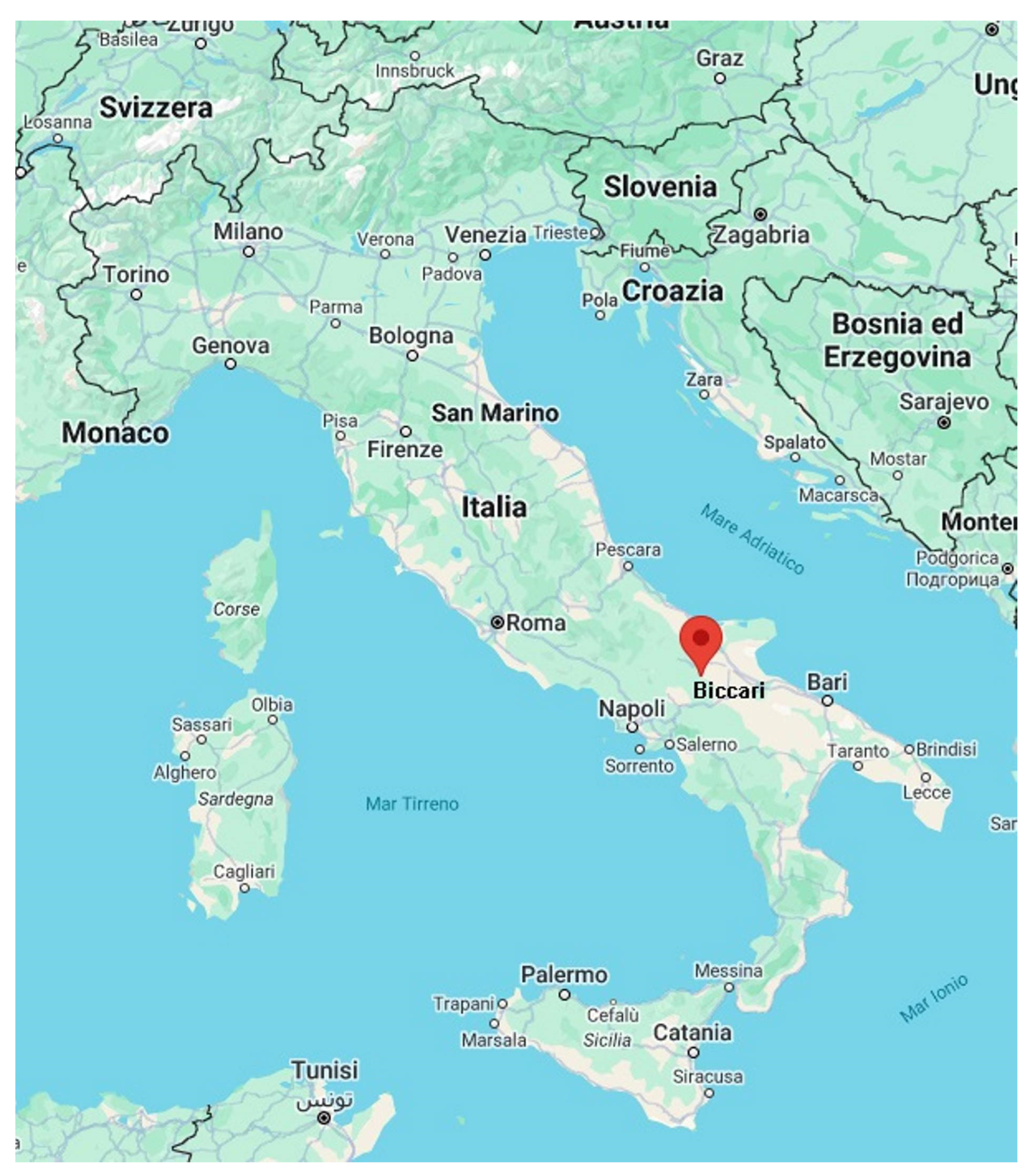
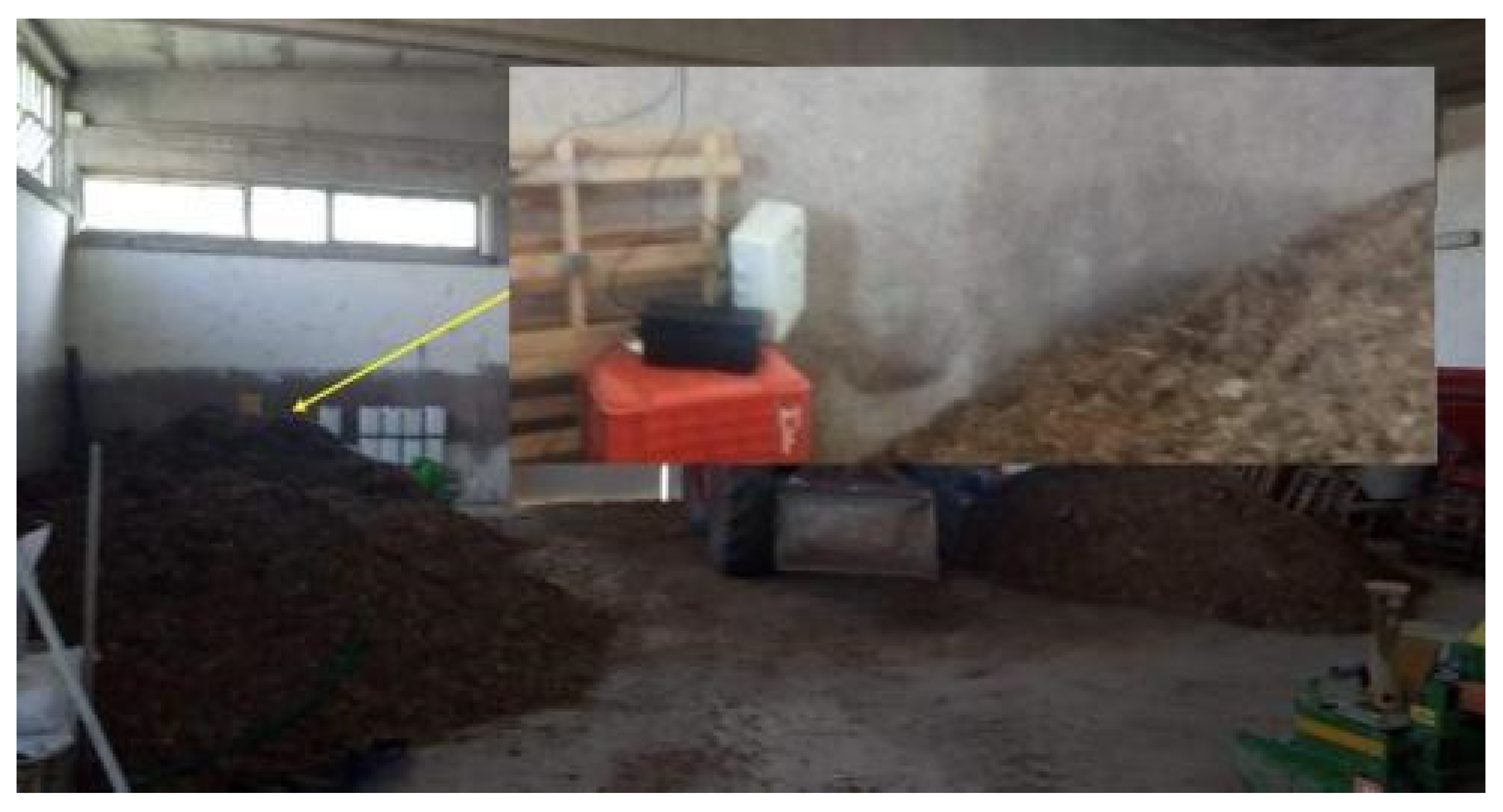
2.1. The Site of the Experiment

One of the experimental trials for the project was held in a rural area of the south of Italy, more specifically, in a location called Biccari (see Figure 1). The treated poultry manure was stored in a depot, the dimensions of which were 20 m × 15 m × 5 m (see Figure 2). The room was accessible by operators and workers and had no forced ventilation systems. Some windows located close to the depot ceiling were left partially opened to ensure a certain amount of natural ventilation. The total area left open was 2.7 m². Moreover, the location was characterized by an unstable and weak Internet signal radio, which allowed us to test a protocol to remotely control the monitoring units. As seen in Figure 2 and Figure 3, the first monitoring unit was placed very close to the manure heaps inside the depot, while the second one was placed outside the depot in its close vicinity.

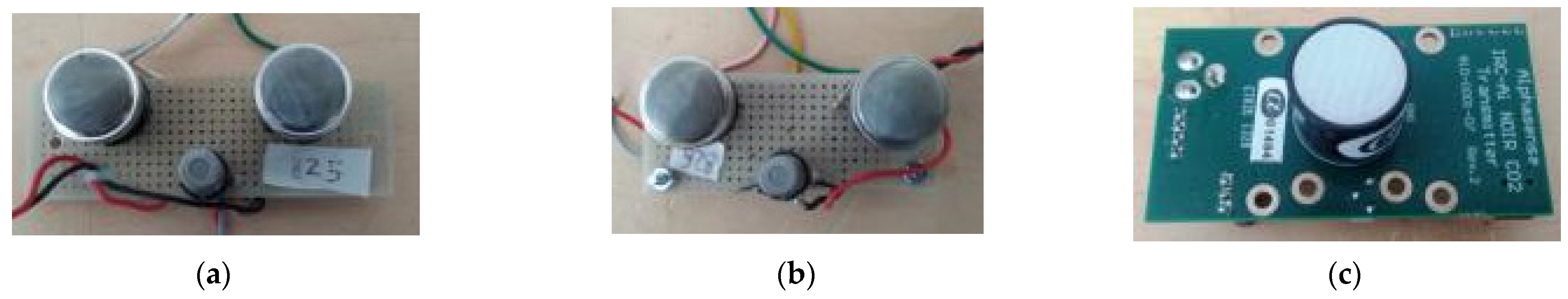
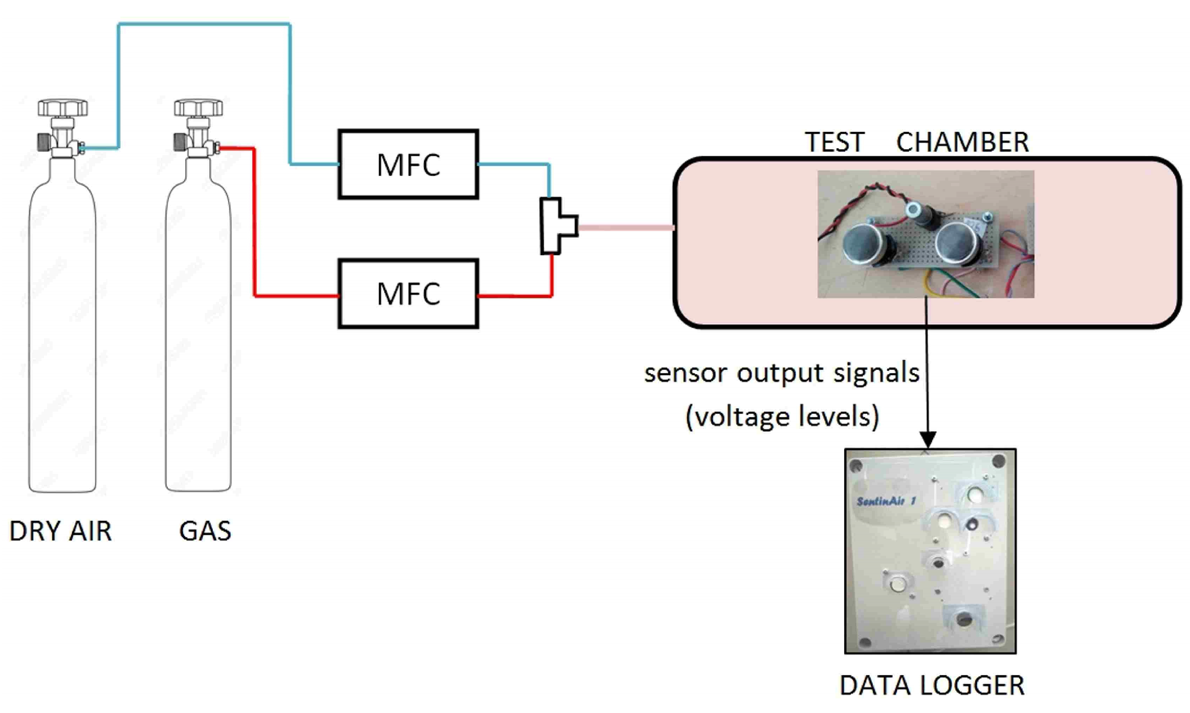
2.2. The LCSs Selected for Gas Monitoring and Their Calibration

As explained earlier, the main gases expected to be emitted by the treated manure were NH₃, CH₄, H₂S, and CO₂; therefore, the LCSs selected for their monitoring were, respectively, the TGS826, the TGS2611, the TGS825, and the IRC-A1. The first three sensors are resistive sensor types by Figaro [40], while the last one is an NDIR sensor by Alphasense [41]. Three main reasons led us to the selection of these types of sensors: the most important one was their affordability; the second one was their small size; and the third one was the absence of cross-sensitivity issues in the use of such sensors. To better clarify this last aspect, let us consider, for example, the TGS826 model: it is sensitive to ammonia, which is the gas target or the gas type for which the sensor has been designed and built, but it is also sensitive to ethanol and iso-butane, which are considered as interfering gases for the sensor. In our case, we did not expect relevant concentrations of these interfering gases; for this reason, we decided to use the TGS826 for ammonia concentration measurements. Similar considerations could be made for the rest of the gas sensors used for this experiment.

The selected set of sensors was installed on both the first monitoring unit inside the depot, and on the second one outside it (see Figure 2 and Figure 3). The CO₂ sensor (called IRC-A1) was purchased with the electronic board to support its operation provided by Alphasense. This board is capable of providing the concentrations of the CO₂ expressed in “ppm” through the USB interface, which we used to connect it with the SentinAir system (see [37,38,39]). The sensor and its support board are sold by the manufacturer as already calibrated; therefore, no further calibration in the laboratory was necessary. On the contrary, the resistive sensors were not available with a support board capable of providing data expressing the measurements of the gas concentrations; thus, it was necessary to design and implement a suitable board to operate them. The working principle of the resistive sensors for gas concentration measurements can be summarized as an electric resistor that can vary its electric conductance depending on the number of gas molecules affecting its sensing surface. The sensing layer of such sensors needs to operate at high temperatures; then, it is necessary to provide electric power to the on-purpose pins of the sensor to activate their heaters. The electronic board implemented to operate them is capable of performing this task and providing an output signal consisting of a DC voltage that can vary by following the variations in the sensor’s electric conductance and the downrange of the gas concentrations (see Figure 4). Both the boards designed for the resistive sensors and the support board for the IRC-A1 sensor are characterized by sizes small enough to be easily integrated and installed in the SentinAir monitoring units.

The analogic signals coming out from the resistive sensors formed the inputs of the interfacing board connected to the SentinAir system [37], which is in charge of converting them into digital data expressing the gas concentrations through its analog-to-digital (A/D) converter. Thus, the resistive sensors TGS825, TGS826, and TGS2611 provided voltage levels as outputs that reflected the gas concentrations experienced by their sensing layer; therefore, they needed to be calibrated in the laboratory for their effective use.

To perform this task, we used gas cylinders with a certified concentration of gas, a mass flow controller (MFC) system to obtain different gas flows, a mixing device to mix the dry air flow with the test gas flow, and a test chamber where the sensors to calibrate were placed. The system composed of these elements was set up by following the scheme depicted in Figure 5.

The calibration of the sensors was performed by exposing them to different known gas concentrations obtained by mixing the flow provided by the MFC regulating the test gas (F_gas), which was NH₃, CH₄, or H₂S depending on the sensors under test, and the flow coming out from the dry air MFC (F_air). To make the different gas concentrations, the MFCs were regulated to provide flows according to the following formulas:

$$\mathrm{C}={\displaystyle \frac{{\mathrm{F}}_{\mathrm{g}\mathrm{a}\mathrm{s}}}{{\mathrm{F}}_{\mathrm{a}\mathrm{i}\mathrm{r}}+{\mathrm{F}}_{\mathrm{g}\mathrm{a}\mathrm{s}}}}$$

(1)

F_tot = F_air + F_gas,

(2)

where F_tot was fixed to 1000 mL/min, and C is the gas concentration expressed in “ppm”.

The output signals coming out from the sensor boards were logged by the SentinAir device and stored in files to use for the subsequent calibration process.

For calibrating the resistive sensors, we injected into the test chamber ten known concentrations of gas alternated with dry air, which is useful for tracking the fluctuation of the sensor “zero levels”, which are the voltages present at the sensor board outputs when there is a gas concentration equal to zero. The “zero levels” and the voltages obtained in correspondence with the various gas concentrations were used to compose a set of data on which it was possible to determine the mathematical law linking the sensor voltages to the gas concentrations. As our purpose was to indicatively assess the gas concentrations emitted by the poultry manure heaps, we reckoned that a linear law could be sufficient for this aim; therefore, given that the linear law can be written as:

C = aV + b,

(3)

where C is the gas concentration expressed in “ppm”, and V is the sensor board voltage expressed in volts. The set of data built as described earlier was useful to calculate the “a” and “b” coefficients present in Formula (3) through the method of linear regression. The software tool used to calculate them was Origin 7.0 by OriginLab.

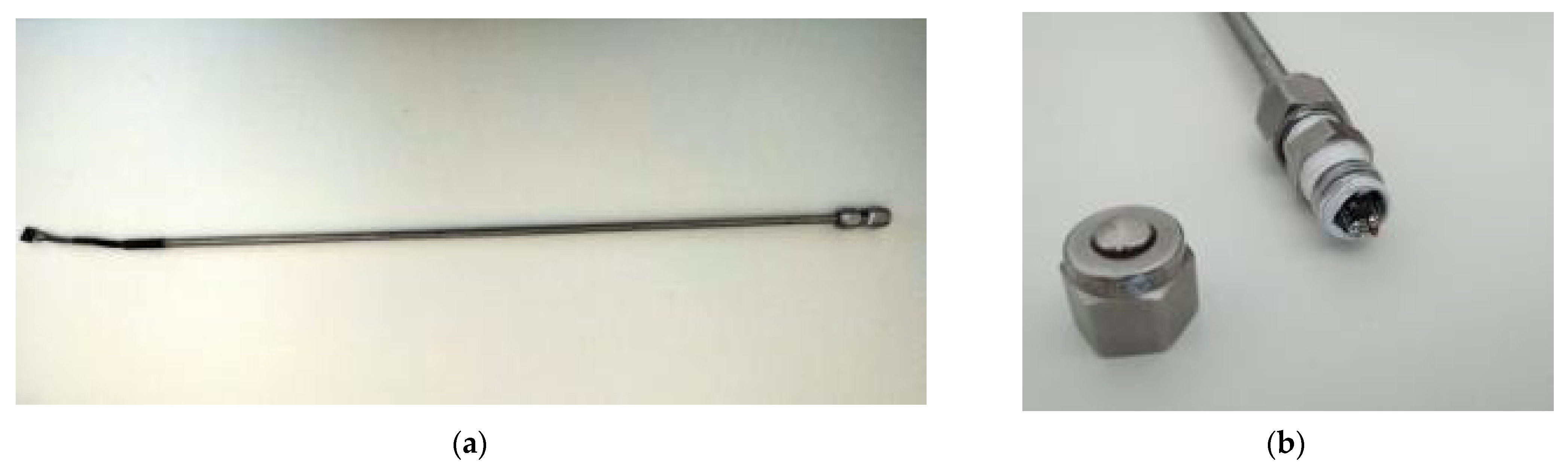
2.3. The Monitoring of the Temperature inside the Manure Heaps and Other Environmental Variables

The monitoring units developed in our laboratory were equipped with sensors to measure the ambient temperature, the ambient relative humidity, and the temperature inside the manure heaps. The monitoring of these variables was useful to understand the drying level of the treated manure and the bio-activity levels inside it.

The sensors used for measuring temperature and relative humidity were the TC1047A by Microchip [42] and the HIH5031 by Honeywell [43], respectively. These sensors are available in a miniaturized case, and they can be directly soldered onto an electronic board to allow a remarkable level of compactness, such as when used with the SentinAir monitoring units (see Figure 6).

For measuring the temperature inside the manure heaps, a temperature probe was deliberately designed and implemented in our laboratory (see Figure 7a,b). The probe was implemented by cutting a steel pipe used for gas pipelines in our laboratory, to which a gas fitting closed by a steel cap was to the tip. The internal diameter of the pipe and the gas fitting where we placed the TC1047A sensor was 4 mm, which is large enough to host the temperature sensor and the wirings necessary to connect it with the SentinAir system.

We selected the material for making the probe to prevent potentially corrosive phenomena that could damage the temperature sensor. Moreover, we thought that the steel forming the probe would ensure a good thermal conductivity that would have favorable results for an accurate temperature measurement.

The calibration of these sensors was not necessary because their manufacturers provide the complete mathematical law linking the sensor signal outputs with the physical quantity to measure.

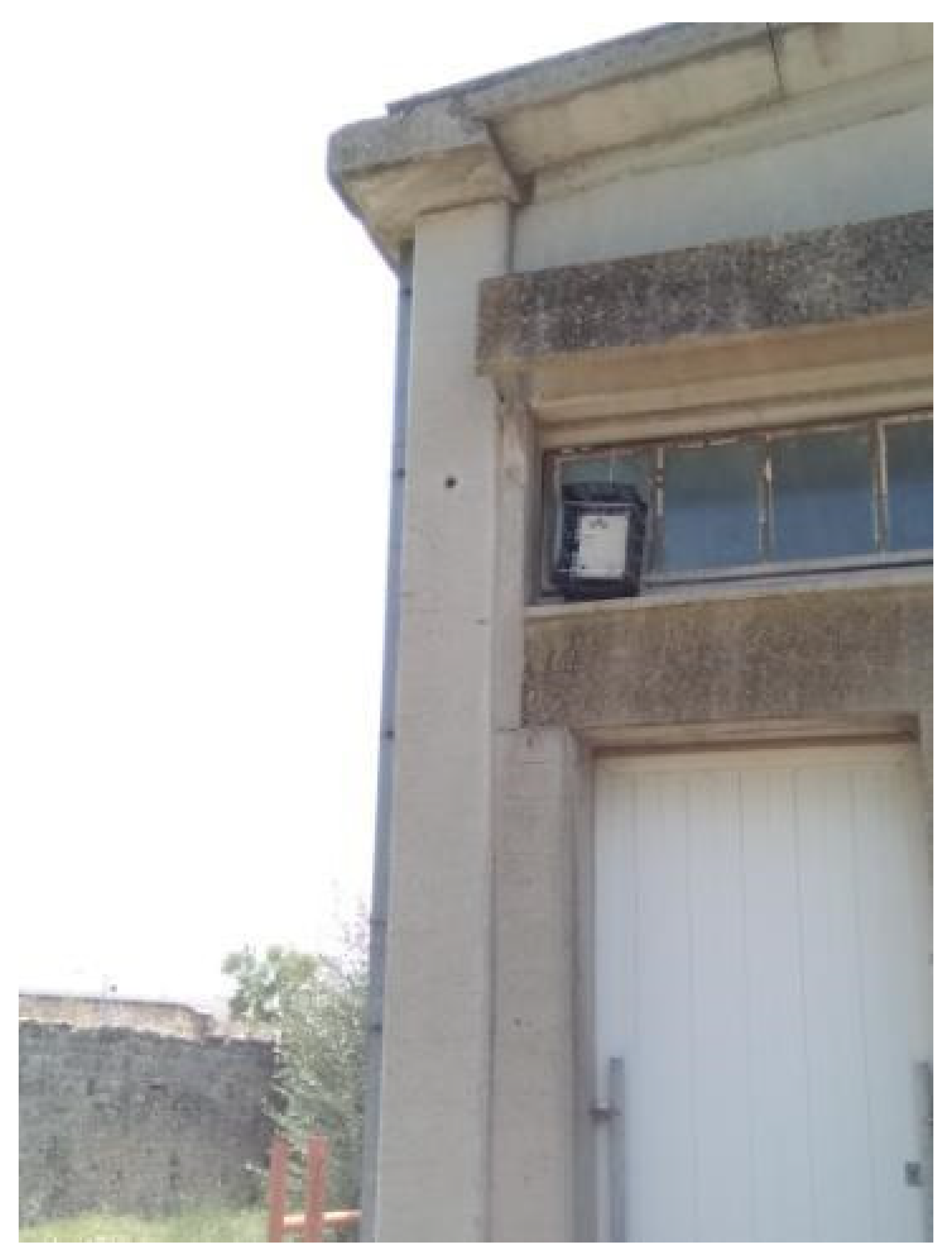
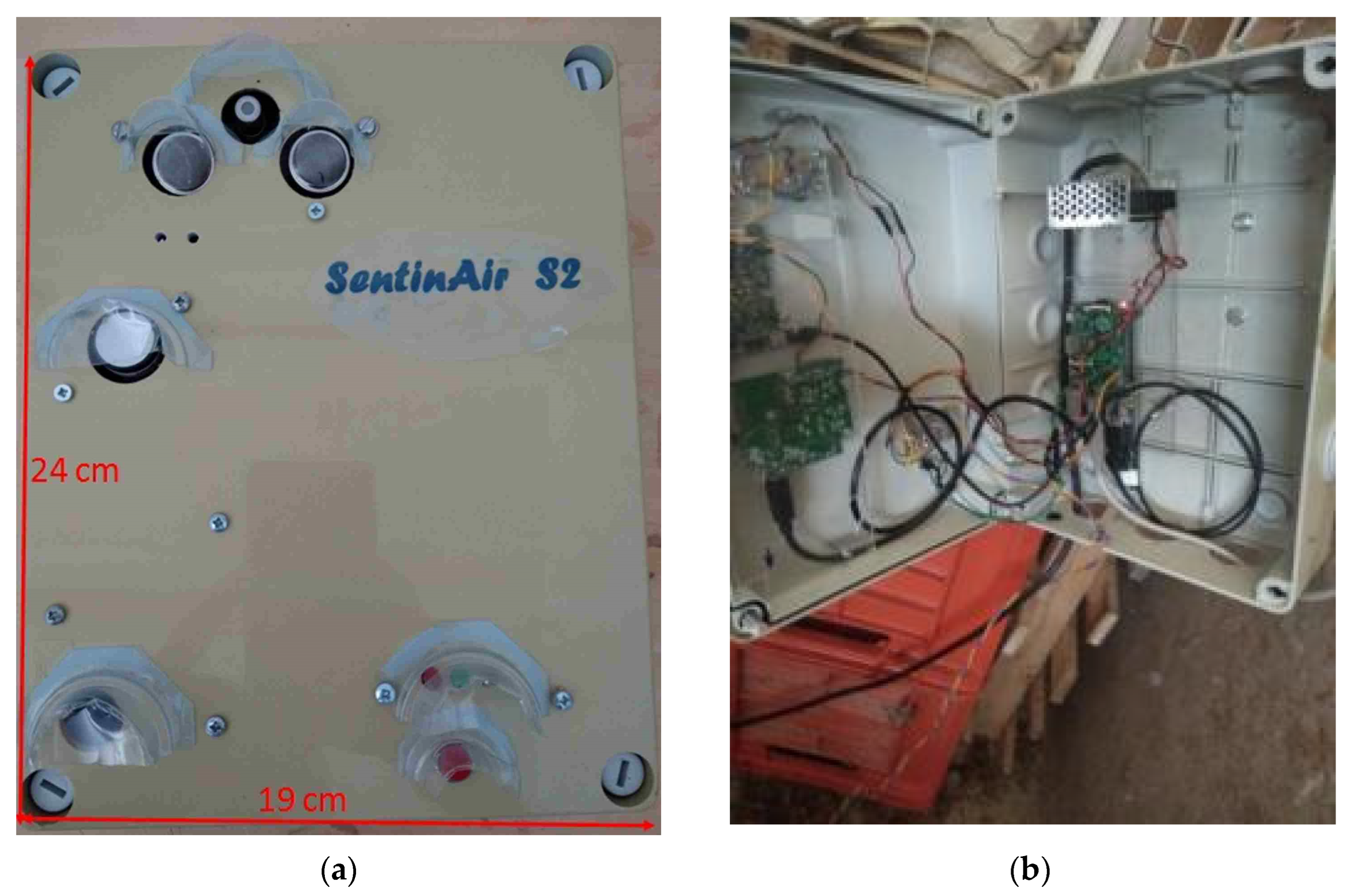
2.4. The Monitoring Unit and the Communication Protocol

The system designed and implemented in our laboratory to carry out the monitoring of the gas emitted by the treated poultry manure and the other variables meaningful for our purposes is a multi-purpose device acting as an LCAQM and as a data logger called SentinAir [37,38,39] (see Figure 8). Some features differentiate SentinAir from other similar devices available on the market or designed by other research groups: the most important are the capability to use a varied range of sensor models, and the capability to be remotely controlled even when deployed in locations where the Internet radio signal is weak and unstable.

The first characteristic is possible due to the hardware featuring the main board of the system and also to the software developed for its operation. The SentinAir main board is a low-cost mini-computer available on the market and called Raspberry 3b+ [44]. It is provided with four USB ports, a serial-TTL port, and an I2C bus through which it is possible to connect different sensors, or other modules developed or adapted for the SentinAir system (see [37,39]). This hardware can operate a heterogeneous variety of sensors and devices because it is managed by the particular software framework developed for the purpose that makes their plug-and-play use possible through the installation of software modules or “device drivers” specific for each sensor or device to use with SentinAir. More details about the SentinAir software can be found in an earlier publication as well as on the GitHub web repository [38,39].

The communication protocol developed in the case of an unstable Internet signal is based on the exchange of e-mail messages containing commands, if directed toward the monitoring unit, or output data, if coming from the monitoring unit. The SentinAir device periodically connects to the given Imap/Smtp servers to search for e-mails sent by the user containing commands. If some such e-mails are found (the system can recognize them by scanning the e-mail subjects), it automatically reads the e-mail, extracts the commands, and then returns the answer by connecting with the given Smtp server. If the connection, the transmission, or the reception of the e-mail messages fails due to an unstable Internet signal, the system performs continuous attempts to rectify the interrupted operation until it succeeds. More details about this communication system can be found on the GitHub web repository and in an earlier article [38,39].

3. Results

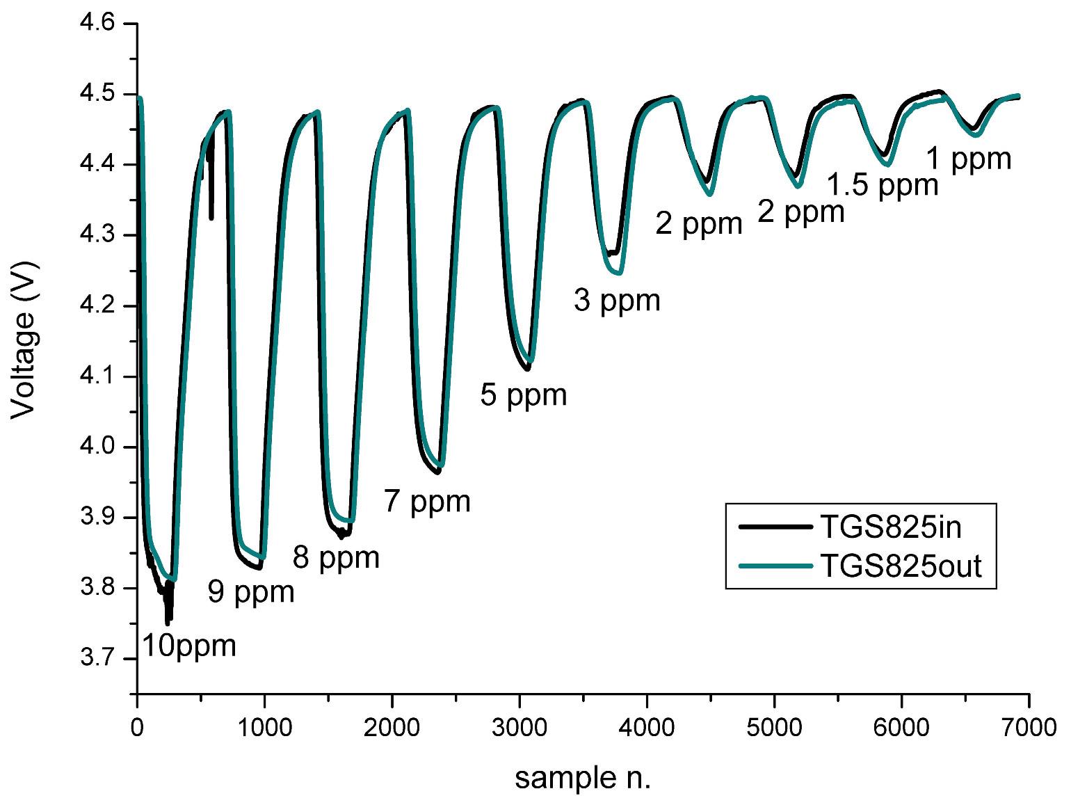
3.1. The Results of the Calibration of the Resistive Gas Sensors in the Laboratory

The resistive sensors used for this experience were calibrated by alternating steps in which a known gas concentration was injected in the test chamber at a flow rate equal to 1000 mL/s for 900 s with steps in which dry air was injected at the same flow rate for the same time (see Figure 9, Figure 10 and Figure 11). Two sets of sensors composed of TGS825, TGS826, and TGS2611 were calibrated under the same conditions. The first set identified by the suffix “in” was later installed in the monitoring unit deployed inside the depot and near the manure heaps, and the second set identified by the suffix “out” was later installed in the monitoring unit deployed outside the depot.

Starting from the data collected through the earlier shown expositions to the target gases, it was possible to make the calibration tables (see

Table 1. The calibration table elaborated for the TGS825 sensor.

H2S Concentrations (ppm)	TGS825in (V)	TGS825out (V)
10	3.78	3.81
9	3.82	3.84
8	3.87	3.89
7	3.96	3.97
5	4.11	4.12
3	4.27	4.24
2	4.37	4.35
2	4.38	4.36
1.5	4.41	4.4
1	4.45	4.44
0	4.48	4.47

,

Table 2. The calibration table elaborated for the TGS826 sensor.

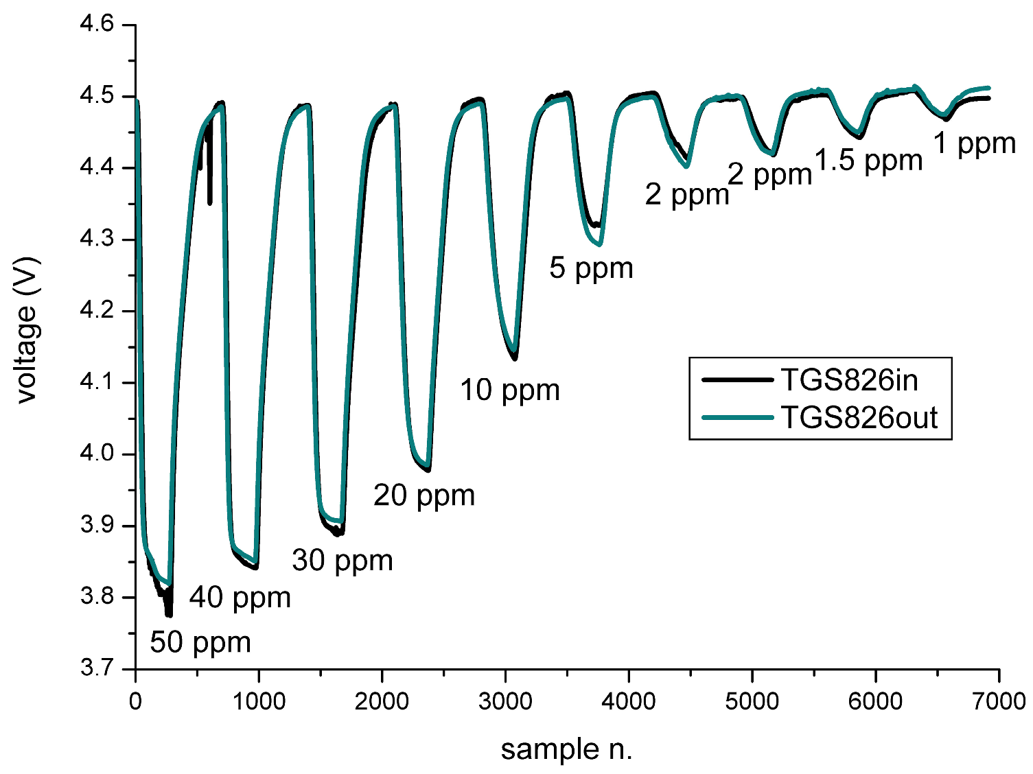
NH3 Concentrations (ppm)	TGS826in (V)	TGS826out (V)
50	3.78	3.82
40	3.84	3.85
30	3.89	3.9
20	3.97	3.99
10	4.13	4.14
5	4.31	4.29
2	4.41	4.4
2	4.41	4.42
1.5	4.44	4.45
1	4.46	4.47
0	4.49	4.49

and

Table 3. The calibration table elaborated for the TGS2611 sensor.

CH4 Concentrations (ppm)	TGS2611in (V)	TGS2611out (V)
100	2.78	2.82
90	3.01	3.04
80	3.29	3.32
70	3.61	3.62
60	3.88	3.89
30	4.06	4.03
15	4.16	4.14
15	4.15	4.15
10	4.21	4.17
8	4.24	4.22
0	4.27	4.26

) whereby the “a” and “b” coefficients of Equation (3) could be calculated for each sensor. The particular trend of the gas in the test chamber during the calibration consisting of more steps of zero gas concentrations allowed us to carry out a preliminary and indicative check on the stability of the sensor “zero level”. Moreover, the repetition of a step with an identical gas concentration gave us rough indications about the repeatability of the measurements performed by such sensors.

The calculation of the coefficients related to Equation (3) for each sensor was performed by using the linear regression algorithm, which provided the results summarized in

Table 4. The results of the resistive sensor calibrations. R² is the coefficient of determination, while the RMSE is the root mean squared error.

Sensor	a (ppm/V)	b (ppm)	R2	RMSE (ppm)
TGS825in	−12.99	58.61	0.993	0.299
TGS825out	−13.85	62.19	0.992	0.331
TGS826in	−61.06	270.77	0.906	5.748
TGS826out	−62.67	278.02	0.894	6.101
TGS2611in	−66.34	294.71	0.918	11.161
TGS2611out	−69.23	305.67	0.915	11.400

.

The coefficients reported in Table 4 were used to modify the software of the monitoring units in order to automatically convert the voltage output signals of the sensors into gas concentrations. This operation allowed us to create a unique database reporting the concentrations of the resistive sensors along with the rest of the sensor set.

3.2. The Results of the On-Field Monitoring

The monitoring of the gas concentrations and the other variables on the site of the experiment lasted 4 months and 2 days. The sampling rate of the measurements was set to 5 min; the sensor readings were used to calculate in real-time the hourly means of such variables and store them in a CSV (comma-separated values) file acting as a local database in the monitoring units. It was possible to gradually download these files from our laboratory thanks to the particular communication protocol earlier described and assemble the pieces composing the database in a unique file available in the Supplementary Materials attached to this document.

The trends of the gas concentrations are shown in Figure 12, Figure 13, Figure 14 and Figure 15, while the trends of the other monitored variables are exposed in Figure 16 and Figure 17. In Figure 14, Figure 15 and Figure 16, some spikes can be observed. We suppose that those values, which are clearly out of the range measured in that period, are just electromagnetic interferences affecting the electronic circuitry of the monitoring units. In particular, we noted that the spikes in the measures only concerned the sensors installed in the monitoring unit inside the depot. The most likely explanation for these data can be ascribed to the presence of electrical switches in the depot and interrupters that could cause electromagnetic spikes when operated.

The trends exposed in Figure 12, Figure 13, Figure 14, Figure 15, Figure 16 and Figure 17 are summarized in

Table 5. The statistics concerning the measurements performed during the experiment.

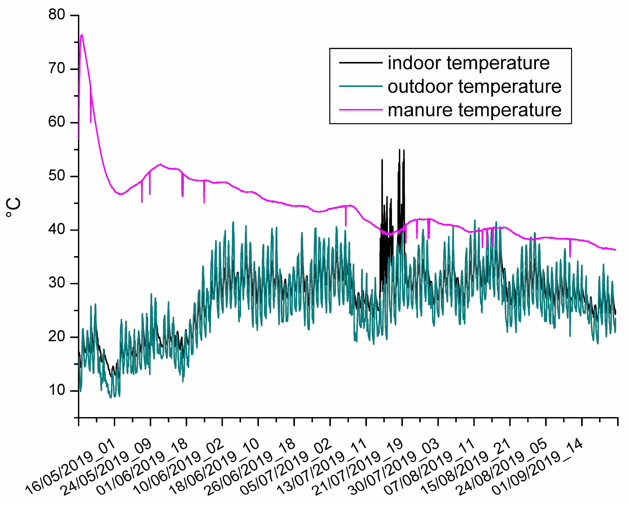
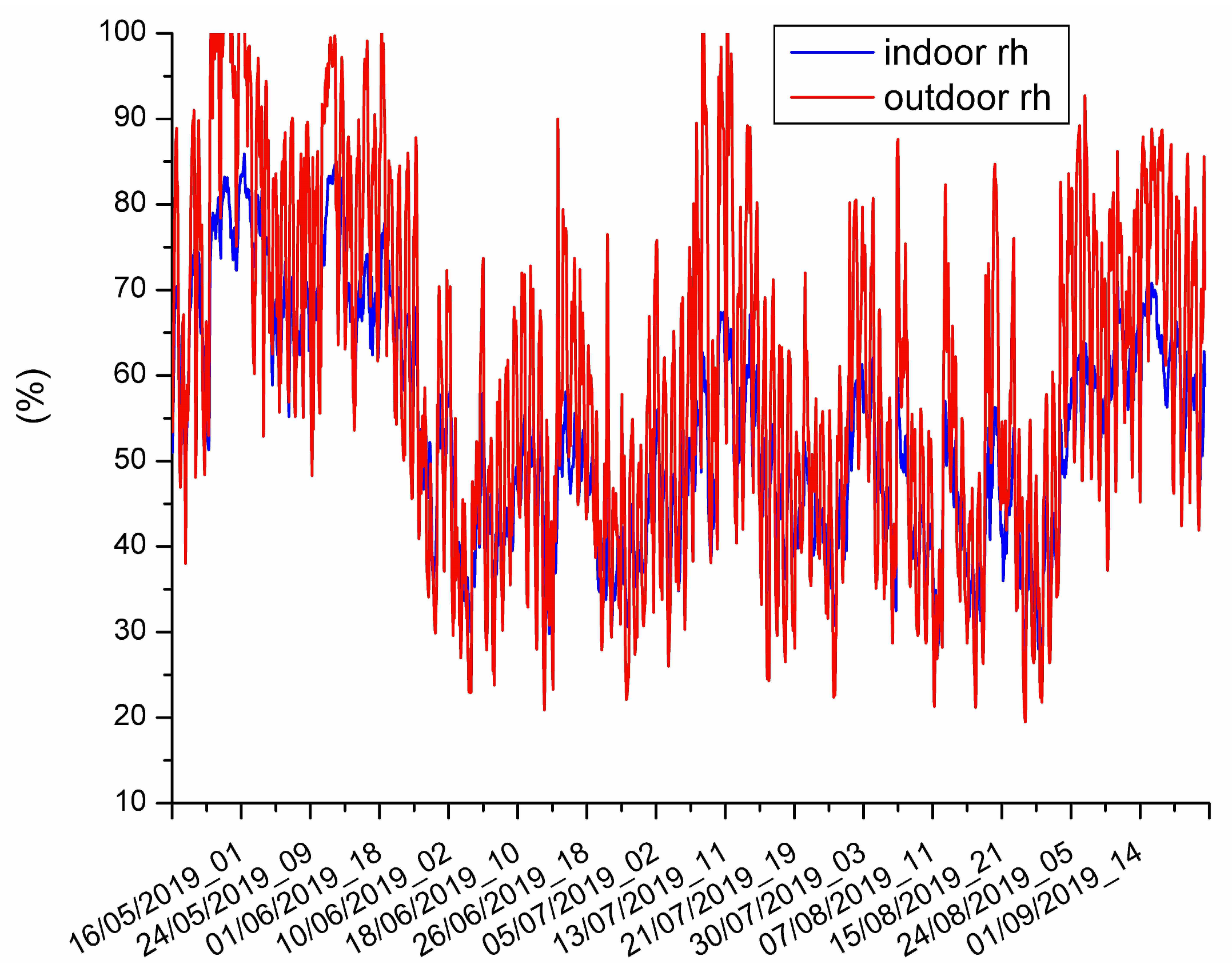
Measurement	Min	Max	Mean	Median
indoor temperature (°C)	12.3	55	27.7	29
outdoor temperature (°C)	8.7	41.8	26.3	26.3
manure temperature (°C)	35	76.4	44.4	43.5
indoor rh (%)	27	86	53	51.3
outdoor rh (%)	19	112	60	57.8
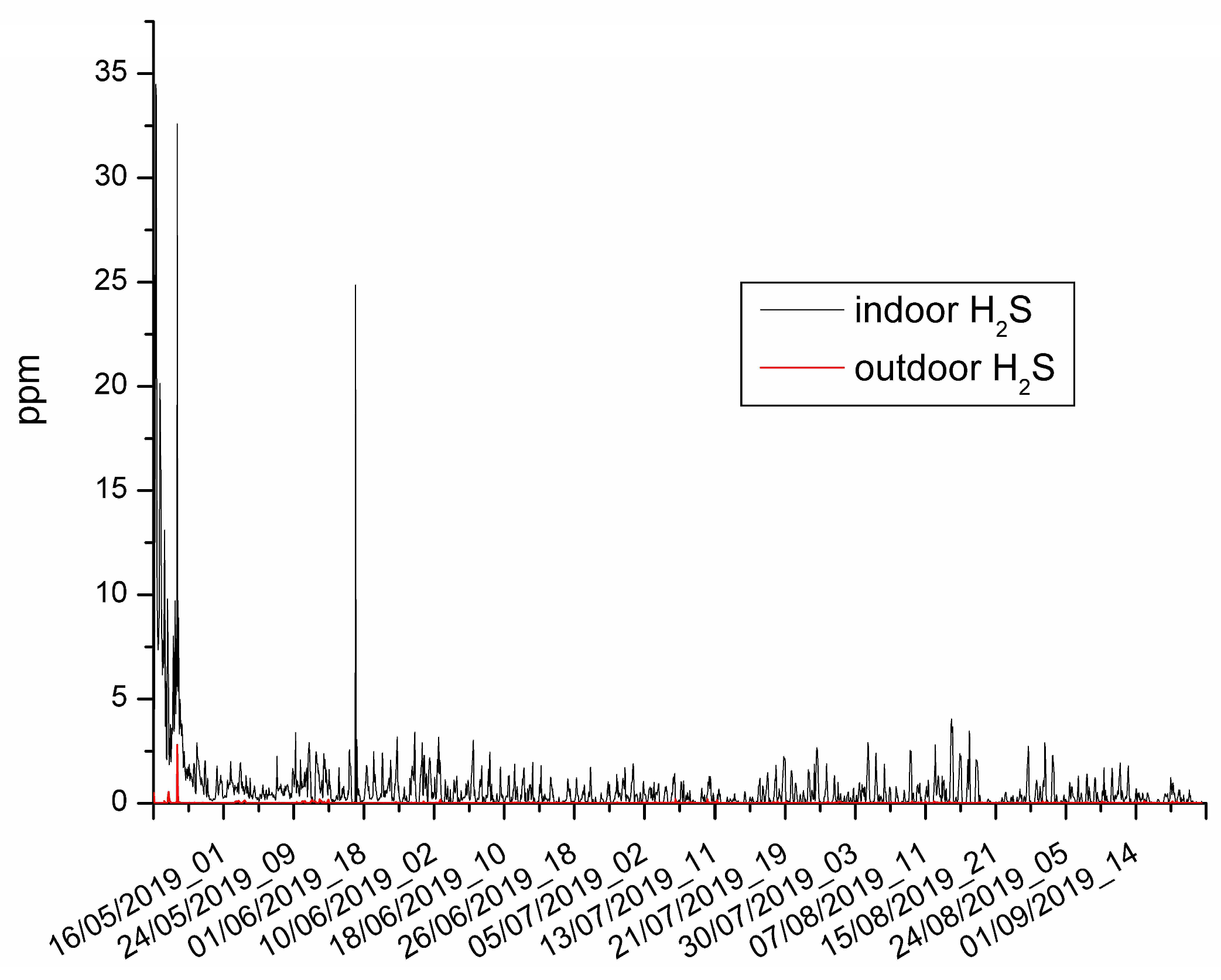
indoor H2S (ppm)	0	34.48	0.72	0.29
outdoor H2S (ppm)	0	2.8	0.03	0.02
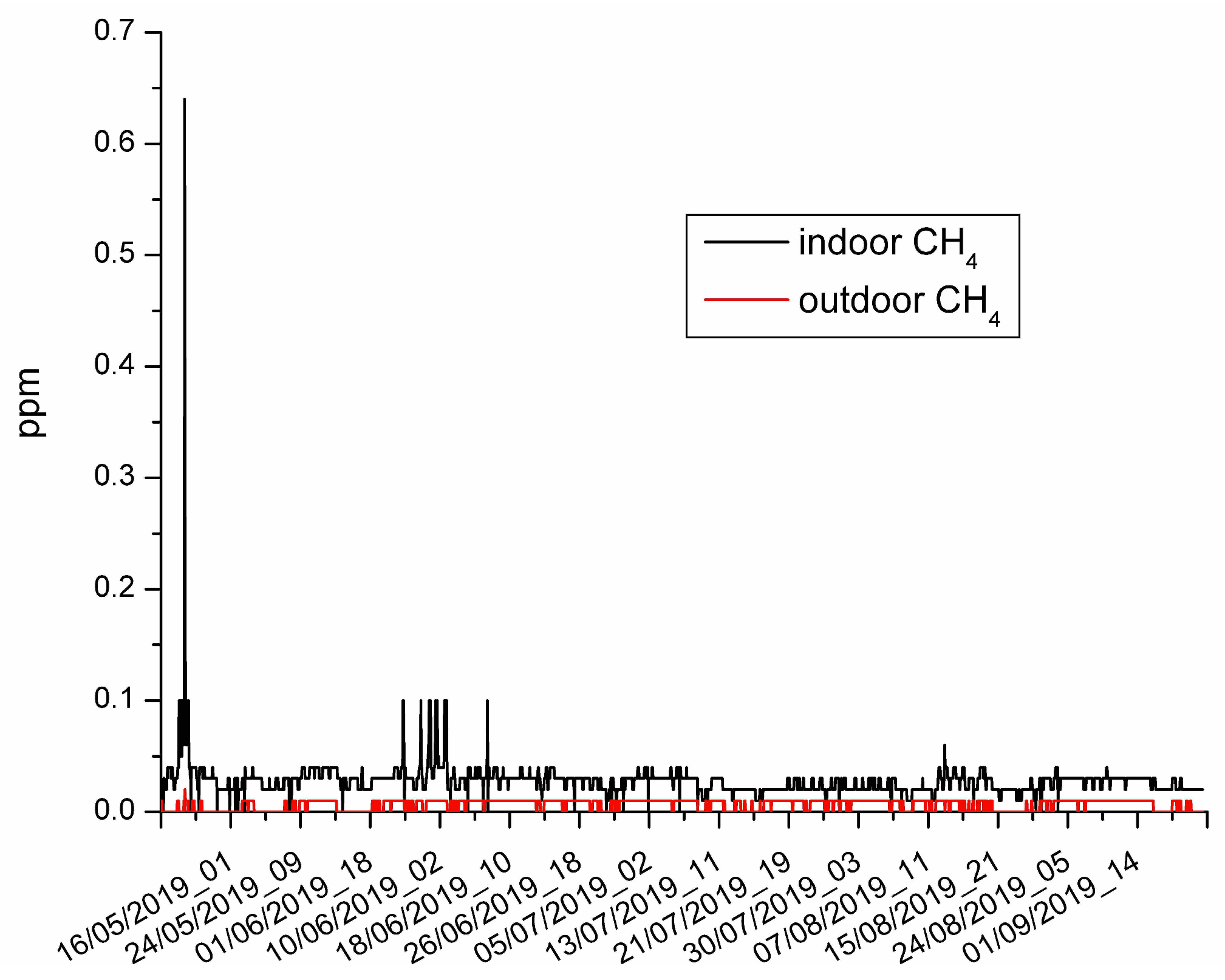
indoor CH4 (ppm)	0	0.64	0.03	0.03
outdoor CH4 (ppm)	0	0.02	0.01	0.01
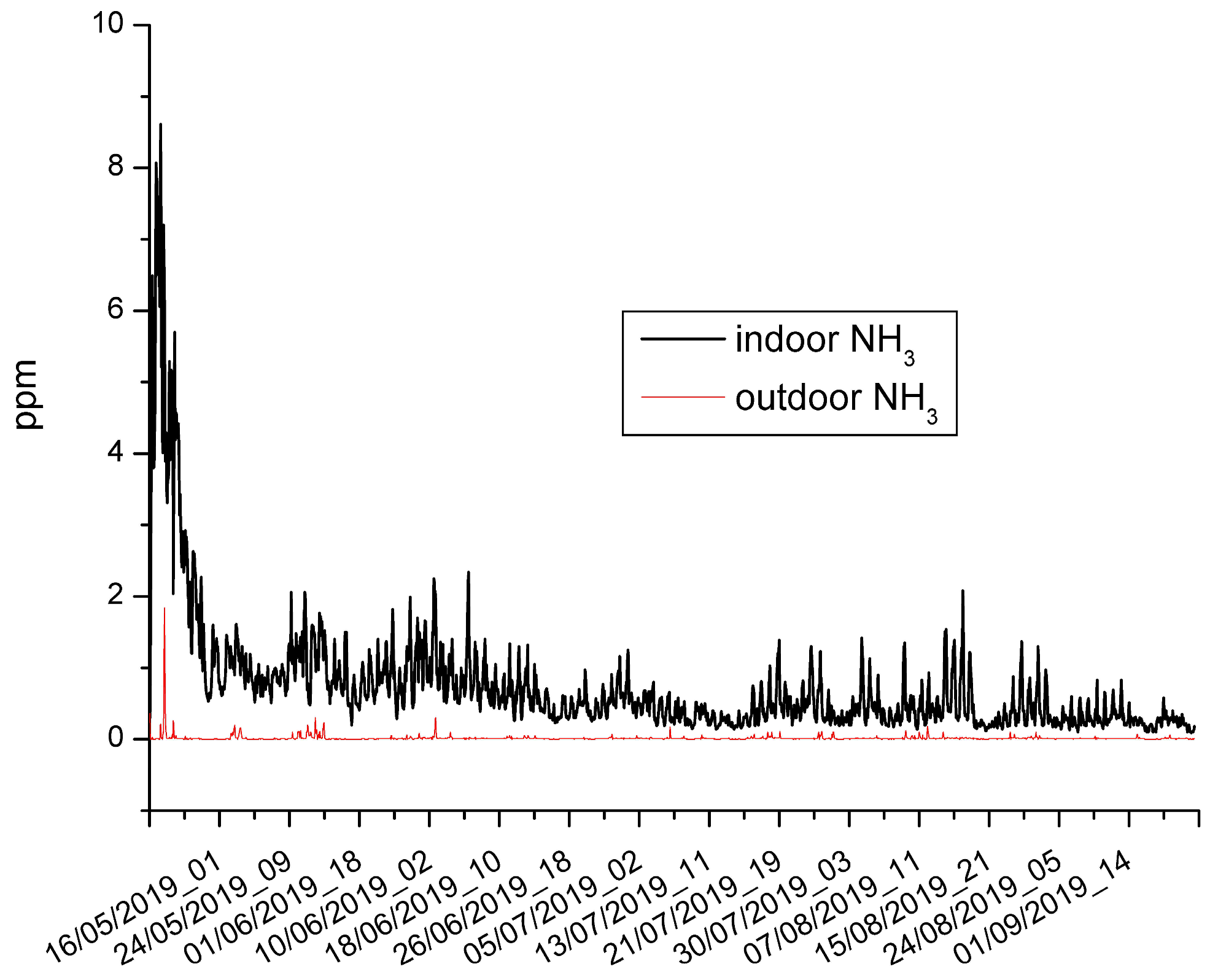
indoor NH3 (ppm)	0.09	8.61	0.74	0.5
outdoor NH3 (ppm)	0	1.84	0.02	0.01
indoor CO2 (ppm)	510	1285	688	666
outdoor CO2 (ppm)	93	567	377	371

, where a more accurate examination of the data concerning the measures can be carried out.

4. Discussion

As concerns the measurements of the gas concentrations, by inspecting Figure 12, Figure 13, Figure 14 and Figure 15 and Table 5, it can be noted that the values measured indoors are always higher than those detected outdoors. This element makes us conclude that the monitoring units actually measured the gases emitted by the treated poultry manure in the depot rather than those coming from possible nearby sources, and also that the instruments worked correctly. The other important consideration is given by the fact that the main gases emitted were CO₂, NH₃, and H₂S, while no remarkable emission of CH₄ could be measured. As a matter of fact, the mean and median values of the CO₂ concentrations were, respectively, 688 ppm and 666 ppm, while the reported concentrations of ammonia and hydrogen sulfide were, respectively, 0.74 ppm, 0.5 ppm, and 0.72 ppm, 0.29 ppm. As expected, the highest values of the main emitted gases were measured in the first 10 days of the experiment, while their concentrations gradually decreased during the rest of the experimentation period.

The temperature measured inside the manure heaps also followed a trend similar to the main gas emitted: in the first 10 days, it ranged from 76 °C to 48 °C, and thereafter, it started to decrease very slowly to values almost always higher than the ones measured in the indoor and outdoor spaces. On the contrary, indoor and outdoor temperatures followed a trend reflecting the seasonal variations of that location: generally increasing from May to August and slowly decreasing from August to September. Temperature trends along with their ranges, means, and median values indicated that the measurements provided by the machines designed in the laboratory were reliable and reflected the actual values. As concerns the relative humidity values, the main relevant elements are given by the mean and median outdoor values higher than the indoor ones, which was expected; meanwhile, we confirmed that the indoor values were adequate for allowing the drying process of the manure heaps.

To the best of our knowledge, very few studies reporting data on the monitoring of gas concentrations emitted during rural activities and performed through LCAQMs can be found. However, even though relevant differences exist, some comparisons can be made with the work of D’Urso et al. [30]. In this study, the potential use of low-cost portable devices for the measurement of ammonia and carbon dioxide concentrations in an open dairy barn was investigated. Three units of the same LCAQM model were used for evaluating their performance against reference instruments in an open barn where some fans were present to ensure forced ventilation. Fifty-seven cows were hosted in a barn which was 55 m long, 20 m wide, and had variable height ranging from 4 m to 7 m. Another significant difference was in the duration of the studies: the experiment performed by D’Urso et al. lasted 5 days, while this one lasted more than 4 months.

The comparison with this study is summarized in

Table 6. Comparison between the measures of CO₂ and NH₃ concentrations found by this study and those found in the work carried out by D’Urso et al. [30]. The data referring to the mean in the study by D’Urso et al. are expressed as a range because three devices were used for the measurements.

Measure	Mean (ppm)	Min (ppm)	Max (ppm)
CO2 (indoor study)	688	510	1285
CO2 ([30] LCAQM)	445–780	450	1400
CO2 ([30] reference)	559–599	480	750
NH3 (indoor study)	0.74	0.09	8.61
NH3 ([30] LCAQM)	0.68–3.63	0	7.1
NH3 ([30] reference)	1.69–3.51	1.4	7.5

. In making the comparison, the measures performed outside the depot are not considered because they express the gas concentrations of the background environment, which is not the focus of this experiment. The main similarity emerging from the data exposed in this table is given by the mean values of measures performed by this study and the LCAQMs used in [30]. It can be noted that the mean values of CO₂ and NH₃ concentrations found in this work fall in the range of values found in [30]. Another element of similarity is given by the range of concentrations measured for both CO₂ and NH₃ through the LCAQMs used in both studies, while a slight difference can be noted between the maximum value of the CO₂ concentration detected by the reference instruments used in the work by D’Urso et al., and the maximum value found by this study.

5. Conclusions

The results of this experiment highlight the feasibility of monitoring the gases emitted during rural activities through low-cost technologies and instruments. Laboratory-made devices were designed and implemented for this purpose, while the calibration of low-cost gas sensors was performed using gas cylinders generating known gas concentrations. The calibration results indicated a good global performance in terms of the coefficient of determination, which ranged from 0.894 to 0.993. The RMSE values found by the calibration process also indicated that the best performance was achieved by the TGS825 sensor (ranging from 0.299 ppm to 0.331 ppm).

The open hardware machine [37] featuring open source software [38] developed in our laboratory proved the effectiveness of the communication protocol based on e-mail exchange for the remote control of the device deployed in areas characterized by a weak and unstable Internet radio signal.

It was also found that the main gases emitted by the treated poultry manure developed in the context of the POREM project were CO₂, NH_3, and H₂S. Their highest concentration values were measured in the first ten days of the experiment, while a long decreasing trend was observed after that period. The temperature inside the treated manure heaps was also monitored using a laboratory-made probe. It showed that the temperature had a peak equal to 76.4 °C, and also that, even for this measurement, the highest values could be observed in the first ten days. These elements indicated that the bio-activation [34] processes were mainly active in the first ten days of the experiment.

A comparison with a previous study [30] concerning the measurement of the concentrations of CO₂ and NH₃ showed interesting similarities, even though some differences in the conditions of the two experiments were present. In particular, we found that the mean of the concentrations related to NH₃ and CO₂ measured inside the depot by this research (respectively, 0.74 ppm and 688 ppm) is in the range of the values found by D’Urso et al. (respectively, 0.68–3.63 ppm and 445–780 ppm) with regard to the LCAQMs measurements.

References

- Kumar, P.; Morawska, L.; Martani, C.; Biskos, G.; Neophytou, M.; Di Sabatino, S.; Bell, M.; Norford, L.; Britter, R. The rise of low-cost sensing for managing air pollution in cities. Environ. Int. 2015, 75, 199–205. [Google Scholar] [CrossRef] [PubMed]
- Snyder, E.G.; Watkins, T.H.; Solomon, P.A.; Thoma, E.D.; Williams, R.W.; Hagler, G.S.; Shelow, D.; Hindin, D.A.; Kilaru, V.J.; Preuss, P.W. The Changing Paradigm of Air Pollution Monitoring. Environ. Sci. Technol. 2013, 47, 11369–11377. [Google Scholar] [CrossRef] [PubMed]
- Karagulian, F.; Barbiere, M.; Kotsev, A.; Spinelle, L.; Gerboles, M.; Lagler, F.; Redon, N.; Crunaire, S.; Borowiak, A. Review of the Performance of Low-Cost Sensors for Air Quality Monitoring. Atmosphere 2019, 10, 506. [Google Scholar] [CrossRef]
- Velasco, A.; Ferrero, R.; Gandino, F.; Montrucchio, B.; Rebaudengo, M. A mobile and low-cost system for environmental monitoring: A case study. Sensors 2016, 16, 710. [Google Scholar] [CrossRef] [PubMed]
- Castell, N.; Dauge, F.R.; Schneider, P.; Vogt, M.; Lerner, U.; Fishbain, B.; Broday, D.; Bartonova, A. Can commercial low-cost sensor platforms contribute to air quality monitoring and exposure estimates? Environ. Int. 2017, 99, 293–302. [Google Scholar] [CrossRef]
- Kang, Y.; Aye, L.; Ngo, T.D.; Zhou, J. Performance evaluation of low-cost air quality sensors: A review. Sci. Total Environ. 2022, 818, 151769. [Google Scholar] [CrossRef]
- Han, I.; Symanski, E.; Stock, T.H. Feasibility of using low-cost portable particle monitors for measurement of fine and coarse particulate matter in urban ambient air. J. Air Waste Manag. Assoc. 2017, 67, 330–340. [Google Scholar] [CrossRef]
- Masic, A.; Bibic, D.; Pikula, B.; Blazevic, A.; Huremovic, J.; Zero, S. Evaluation of optical particulate matter sensors under realistic conditions of strong and mild urban pollution. Atmos. Meas. Tech. 2020, 13, 6427–6443. [Google Scholar] [CrossRef]
- Guidi, V.; Carotta, M.C.; Fabbri, B.; Gherardi, S.; Giberti, A.; Malagù, C. Array of sensors for detection of gaseous malodors in organic decomposition products. Sens. Actuators B Chem. 2012, 174, 349–354. [Google Scholar] [CrossRef]
- Suriano, D.; Rossi, R.; Alvisi, M.; Cassano, G.; Pfister, V.; Penza, M.; Trizio, L.; Brattoli, M.; Amodio, M.; De Gennaro, G. A Portable Sensor System for Air Pollution Monitoring and Malodours Olfactometric Control. In Sensors and Microsystems: AISEM 2011 Proceedings; Lecture Notes in Electrical Engineering; Springer: Boston, MA, USA, 2012; Volume 109. [Google Scholar]
- Abulude, F.O.; Suriano, D.; Oluwagbayide, S.D.; Akinnusotu, A.; Abulude, I.A.; Awogbindin, E. Study on indoor pollutants emission in Akure, Ondo State, Nigeria. Arab. Gulf J. Sci. Res. 2023; ahead of print. [Google Scholar] [CrossRef]
- Suriano, D.; Penza, M. Assessment of the Performance of a Low-Cost Air Quality Monitor in an Indoor Environment through Different Calibration Models. Atmosphere 2022, 13, 567. [Google Scholar] [CrossRef]
- Suriano, D.; Prato, M. An Investigation on the Possible Application Areas of Low-Cost PM Sensors for Air Quality Monitoring. Sensors 2023, 23, 3976. [Google Scholar] [CrossRef] [PubMed]
- Trizio, L.; Brattoli, M.; De Gennaro, G.; Suriano, D.; Rossi, R.; Alvisi, M.; Cassano, G.; Pfister, V.; Penza, M. Application of artificial neural networks to a gas sensor-array database for environmental monitoring. In Sensors and Microsystems; Springer: Boston, MA, USA, 2012; pp. 139–144. [Google Scholar]
- Cavaliere, A.; Carotenuto, F.; Di Gennaro, F.; Gioli, B.; Gualtieri, G.; Martelli, F.; Matese, A.; Toscano, P.; Vagnoli, C.; Zaldei, A. Development of Low-Cost Air Quality Stations for Next Generation Monitoring Networks: Calibration and Validation of PM2.5 and PM10 Sensors. Sensors 2018, 18, 2843. [Google Scholar] [CrossRef] [PubMed]
- Bigi, A.; Mueller, M.; Grange, S.K.; Ghermandi, G.; Hueglin, C. Performance of NO, NO2 low cost sensors and three calibration approaches within a real world application. Atmos. Meas. Tech. 2018, 11, 3717–3735. [Google Scholar] [CrossRef]
- Pitarma, R.; Marques, G.; Ferreira, B.R. Monitoring Indoor Air Quality for Enhanced Occupational Health. J. Med. Syst. 2017, 41, 23. [Google Scholar] [CrossRef]
- Zhang, H.; Srinivasan, R.; Ganesan, V. Low Cost, Multi-Pollutant Sensing System Using Raspberry Pi for Indoor Air Quality Monitoring. Sustainability 2021, 13, 370. [Google Scholar] [CrossRef]
- Jo, J.; Jo, B.; Kim, J.; Kim, S.; Han, W. Development of an IoT-Based Indoor Air Quality Monitoring Platform. J. Sens. 2020, 2020, 8749764. [Google Scholar] [CrossRef]
- Tryner, J.; Phillips, M.; Quinn, C.; Neymark, G.; Wilson, A.; Jathar, S.H.; Carter, E.; Volckens, J. Design and testing of a low-cost sensor and sampling platform for indoor air quality. Build. Environ. 2021, 206, 108398. [Google Scholar] [CrossRef]
- Abraham, S.; Li, X. A cost-effective wireless sensor network system for indoor air quality monitoring applications. Procedia Comput. Sci. 2014, 34, 165–171. [Google Scholar] [CrossRef]
- Aleixandre, M.; Gerboles, M. Review of small commercial sensors for indicative monitoring of ambient gas. Chem. Eng. Trans. 2012, 30, 169–174. [Google Scholar]
- Spinelle, L.; Gerboles, M.; Kok, G.; Persijn, S.; Sauerwald, T. Review of Portable and Low-Cost Sensors for the Ambient Air Monitoring of Benzene and Other Volatile Organic Compounds. Sensors 2017, 17, 1520. [Google Scholar] [CrossRef]
- Devkota, J.; Ohodnicki, P.R.; Greve, D.W. SAW Sensors for Chemical Vapors and Gases. Sensors 2017, 17, 801. [Google Scholar] [CrossRef] [PubMed]
- Mandal, D.; Banerjee, S. Surface Acoustic Wave (SAW) Sensors: Physics, Materials, and Applications. Sensors 2022, 22, 820. [Google Scholar] [CrossRef] [PubMed]
- Penza, M.; Rossi, R.M.; Alvisi, M.; Aversa, P.; Cassano, G.B.; Suriano, D.; Benetti, M.; Cannata’, D.; Di Pietrantonio, F.; Verona, E. SAW Gas Sensors with Carbon Nanotubes Films. In Proceedings of the IEEE Ultrasonics Symposium, Beijing, China, 2–5 November 2008; pp. 1850–1853. [Google Scholar]
- Han, T.; Nag, A.; Mukhopadhyay, S.C.; Xu, Y. Carbon nanotubes and its gas-sensing applications: A review. Sens. Actuators A Phys. 2019, 291, 107–143. [Google Scholar] [CrossRef]
- Cross, E.S.; Williams, L.R.; Lewis, D.K.; Magoon, G.R.; Onasch, T.B.; Kaminsky, M.L.; Worsnop, D.R.; Jayne, J.T. Use of electrochemical sensors for measurement of air pollution: Correcting interference response and validating measurements. Atmos. Meas. Tech. 2017, 10, 3575–3588. [Google Scholar] [CrossRef]
- Mead, M.I.; Popoola, O.A.M.; Stewart, G.B.; Landshoff, P.; Calleja, M.; Hayes, M.; Baldovi, J.J.; McLeod, M.W.; Hodgson, T.F.; Dicks, J.; et al. The use of electrochemical sensors for monitoring urban air quality in low-cost, high-density networks. Atmos. Environ. 2013, 70, 186–203. [Google Scholar] [CrossRef]
- D’Urso, P.R.; Arcidiacono, C.; Cascone, G. Assessment of a Low-Cost Portable Device for Gas Concentration Monitoring in Livestock Housing. Agronomy 2023, 13, 5. [Google Scholar] [CrossRef]
- Janke, D.; Bornwin, M.; Coorevits, K.; Hempel, S.; van Overbeke, P.; Demeyer, P.; Rawat, A.; Declerck, A.; Amon, T.; Amon, B. A Low-Cost Wireless Sensor Network for Barn Climate and Emission Monitoring—Intermediate Results. Atmosphere 2023, 14, 1643. [Google Scholar] [CrossRef]
- Woutersen, A.; de Ruiter, H.; Wesseling, J.; Hendricx, W.; Blokhuis, C.; van Ratingen, S.; Vegt, K.; Voogt, M. Farmers and Local Residents Collaborate: Application of a Participatory Citizen Science Approach to Characterising Air Quality in a Rural Area in The Netherlands. Sensors 2022, 22, 8053. [Google Scholar] [CrossRef]
- Seesaard, T.; Goel, N.; Kumar, M.; Wongchoosuk, C. Advances in gas sensors and electronic nose technologies for agricultural cycle applications. Comput. Electron. Agric. 2022, 193, 106673. [Google Scholar] [CrossRef]
- POREM Project Webpage. Available online: https://webgate.ec.europa.eu/life/publicWebsite/project/LIFE17-ENV-IT-000333/poultry-manure-based-bioactivator-for-better-soil-management-through-bioremediation (accessed on 28 June 2024).
- Von Essen, S.G.; Auvermann, B.W. Health effects from breathing air near CAFOs for feeder cattle or hogs. J. Agromedicine 2005, 10, 55–64. [Google Scholar] [CrossRef]
- Akter, S.; Cortus, E.L. Comparison of Hydrogen Sulfide Concentrations and Odor Annoyance Frequency Predic-tions Downwind from Livestock Facilities. Atmosphere 2020, 11, 249. [Google Scholar] [CrossRef]
- Suriano, D. A portable air quality monitoring unit and a modular, flexible tool for on-field evaluation and calibration of low-cost gas sensors. HardwareX 2021, 9, e00198. [Google Scholar] [CrossRef] [PubMed]
- Suriano, D. SentinAir system software: A flexible tool for data acquisition from heterogeneous sensors and devices. SoftwareX 2020, 12, 100589. [Google Scholar] [CrossRef]
- SentinAir GitHub Repository. Available online: https://github.com/domenico-suriano/SentinAir (accessed on 7 July 2024).
- Figaro Website. Available online: https://www.figarosensor.com/ (accessed on 7 July 2024).
- Alphasense Website. Available online: https://www.alphasense.com/ (accessed on 7 July 2024).
- Microchip Website. Available online: https://www.microchip.com/ (accessed on 7 July 2024).
- Honeywell Website. Available online: https://www.honeywell.com/ (accessed on 7 July 2024).
- Raspberrypi Website. Available online: https://www.raspberrypi.com/ (accessed on 7 July 2024).