Abstract
Pressure reducing valves (PRV) are widely used to enhance the performance of water distribution networks. Recently, PRVs have tended towards more sophisticated devices to realize complex control strategies. The present work compares network performances achieved with different PRV control methodologies considering variable demand conditions. A widely analyzed water distribution network is modeled using EPANET and used to simulate the PRV operation. The results show the effectiveness of the different control strategies, highlighting the amount of saved water, the pressure deficit occurring in critical nodes, and the power dissipated by the valve that can be potentially recovered using pumps as turbines or other emerging energy recovery technologies.
1. Introduction
Pressure reducing valves (PRV) are widely diffused devices in water distribution networks (WDNs). They are used to implement pressure management strategies aimed at improving the performance of the network from several points of view, ranging from improving the efficiency of the network to improving service to users. Probably, one of the most interesting ones for WDN managers for its proven effectiveness, is the potential reduction in water leakages [1]. Leakage has been proved to be directly related to the pressure in pipelines. Thus, the control, and basically the reduction, of the pressure in the pipelines allows an effective reduction of the leakages. One widely diffused pressure management strategy for leakage reduction consists of the creation of district metered areas (DMA) that require the installation of a proper PRV at the entrance of the district to operate pressure regulation [2,3,4]. From the technologic point of view, PRVs in recent years have tended towards more responsive and dynamic devices. Standard PRVs can rely usually on a single setting value, which prevents the introduction of sophisticated pressure control strategies. Recently, the use of electronic controllers has been proposed to adjust the setting of the PRV. This solution allowed the introduction of real-time control (RTC) strategies that require the PRV setting to be updated on the basis of a measure made at a remote critical node. This methodology allows the setting of the PRV to be always optimal [5] to minimize the pressure and leakages in the network. Often, the introduction of PRV in a network is coupled with energy recovery; in fact, the energy dissipated by the valve can be potentially exploited using energy recovery systems such as pumps as turbines (PAT) or other energy conversion machinery [6,7,8,9].
Although PRVs are widely studied in literature, as in [10,11,12,13], where their function has been extensively analyzed, few works quantitatively compare the effectiveness of different strategies of regulations that can be realized using different types of PRV. The present work investigated the advantages that can be obtained using PRV equipped with different options for pressure regulation. In particular:
- Standard PRV (C-PRV), that allows a single constant set point for pressure;
- Time-dependent PRV (T-PRV), that allows the tuning of the set point based on the time of day;
- Remote-control PRV (R-PRV), that allows a set point regulation based on the pressure measured in a remote node of the network. In this case, the time control frequency considered is one minute.
The effectiveness of each different type of PRV was considered when an oscillating and varying demand is set in each node of the network. The distribution network model used for the scope is the widely studied network presented firstly by Jowitt and Xu (1990) [14]. The performance of the different pressure regulation methodologies will be compared on the basis of leakage reduction, of the pressure deficit at the critical node and of the energy dissipated by the valve that represents a potential for energy recovery.
2. Materials and Methods
The study is based on demand-driven hydraulic analysis performed using the EPANET–MATLAB toolkit [15], a MATLAB library developed to use EPANET in the MATLAB framework.
The network used in the study is characterized by 25 nodes highly interconnected and supplied by three reservoirs placed on the west side of the network. The PRV is introduced in the section suggested in the work of [16], i.e., between node #12 and #13. For more detailed information about the network, reference can be made to [14,16]. In Figure 1a, a scheme of the network with the valve location is shown.
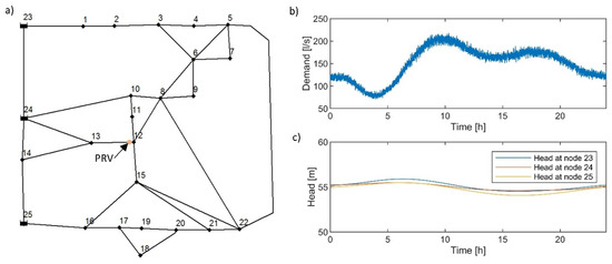
Figure 1.
(a) Scheme of the network with indication of the installation point for the PRV. (b) Total demand as a function of day hours. (c) Head at the fixed head nodes during day hours.
A residential demand has been generated at each node with the bottom-up stochastic approach proposed firstly by [17]. The number of users for each node was calculated on the basis of the base demand of the node and considering an average daily demand per person equal to 400 L for a total of about 30,000 users served by the network. The base demands of the nodes are the ones considered in [16]. For the generation of the oscillating demand, the parameters suggested in [11] were used, i.e., a minimum intervention time defined as a function of the demand pattern with a minimum of 1.5 min and a maximum of 2.5 min during night hours. An event duration of 20 s and an average intensity of 0.1 L/s were considered. The distributions obtained for each user were then aggregated to obtain the resulting oscillating demand for each node for each minute. In Figure 1b, the resulting oscillating demand is shown as a function of day hours. The head of the reservoirs at nodes #23, #24, and #25 follows the curves shown in Figure 1c that were obtained by interpolating the condition suggested in [14] where they are defined with a bi-hourly frequency.
The leakage flow rate of the network is approximated as a function of the emitter coefficient , defined at each node j and of the pressure at the node j [16].
where is the leakage concentrated at the node j, is the pressure at the node j and is the exponent defined according to literature to 1.18.
The emitter coefficient of the node can be calculated as:
where is a characteristic of the junction i connected to the node j, is its length, m is the number of junctions connected to the node j. In the present case, is considered constant for each junction.
The present work compares different control methods achievable using different kinds of PRVs. The scenarios considered are summarized in Table 1. The three different control methods considered, C-PRV, T-PRV, and R-PRV, differ for the different time control periods, which goes from one day for the C-PRV method to one minute for the R-PRV method. The setting of the PRV in all the cases considered is calculated as the setting to obtain a minimum pressure of 30 m in every node in each time control period. Usually, control strategies based on time, such as T-PRV, are set on the basis of the average typical day using a suitable margin. The condition considered in the present work investigates the best performance, i.e., where the pressure at the critical node in each time period reaches exactly 30 m. The most sophisticated pressure control method, R-PRV, can be realized in a real environment using, for example, the methods suggested in [18] and applied in [19] or the method suggested in [20] based on the prevision of the shutter position, of the resistance, or of the head loss associated with the setting of the valve and on the pressure monitored at the critical node. In the present work, the effects of network–valve interactions are neglected. In this way, the computed behavior of the R-PRV expresses the ideal maximum performance achievable with the real-time control of the valve.

Table 1.
List and characteristics of the simulated scenarios.
To assess the effect of demand variation, two cases with an increased demand of 10% and a reduced demand of 20% with respect to the base condition have been performed. In these cases the PRV settings have been maintained equal to the base condition for the C-PRV and T-PRV methods. The setting of the R-PRV is instead calculated on the basis of the actual demand condition and updated at each control period.
To evaluate the performance of the pressure regulation in the network, the relative pressure deficit is calculated. A negative value of indicates a pressure at the node below the limit of 30 m. The relative pressure deficit is calculated as follows:
where is the head at node j and is the limit imposed for head in this case equal to 30 m. The minimum relative pressure deficit for a certain scenario is defined as . A negative value of expresses the occurrence of pressure deficit condition in the network for the considered scenario.
3. Results
The results of the analysis of the several considered scenarios are reported in Figure 2. The results in case of constant setting regulation are shown in Figure 2a. In this case, the pressure at the critical node, which is #21, oscillates with a minimum of 30 m around 10 a.m. The T-PRV case where the PRV setting is adjusted hourly is shown in Figure 2b. It can be noticed that both the setting pressure and the critical node pressure show discontinuity at the end of every hour and the head at the critical node reaches the limit of 30 m every hour. The R-PRV case, where the setting of the PRV is updated every minute, is shown in Figure 2c. In this case, the pressure at the critical node is constant and equal to the limit of 30 m.
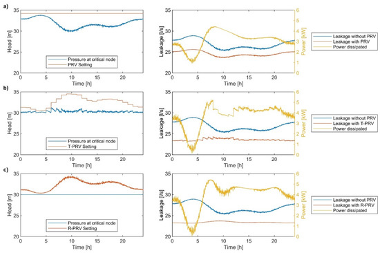
Figure 2.
Results of the simulations with base demand pattern for: (a) constant setting, C-PRV mode; (b) hourly variable setting control, T-PRV mode; (c) real-time setting control, R-PRV mode. On the left, the setting and the critical node pressure are reported. On the right, the leakage flow without and with the PRV are reported together with the power dissipated through the PRV.
By analyzing the plots on the right side of Figure 2, it can be observed that the leakage is considerably reduced due to the introduction of any kind of PRV. Indeed, the leakage without any PRV installed (represented by the blue lines) is always higher than the leakage flow rate calculated after installing any of the PRVs considered. The use of a valve with a constant setting allows a reduction of 9.5%, which corresponds to a saving of more than 120 m3 of water daily. The use of a setting optimized each hour increases the saving up to 13%. Furthermore, the use of a real-time setting that updates the setting of the valve each minute leads to a further 1% saving. The results and the comparison between the different control modes are reported in Table 2.
Table 2.
Leakage volume, potential recoverable power, and pressure deficit at a critical node for base demand pattern and demand pattern increased by 10% and decreased by 20%. The values in brackets are percentages relative to the “No PRV” case.
Regarding the evaluation of the energy that is dissipated in the PRV and that can potentially be recovered, the case with constant setting shows an average dissipated power of 3.1 kW with an increase of 19% in the case of hourly adjustment of the setting and of a further 6% in case of R-PRV, which corresponds to a total of 3.9 kW. Clearly, these powers represent only a potential because the process of transformation from hydraulic power to electric power has a specific efficiency that depends on the device used for the conversion. The available power changes widely during the day as shown in Figure 2. Especially, during the night, the power reaches the minimum value, which for the T-PRV and R-PRV cases is close to zero. This limiting case occurs when the pressure in the network increases due to the night-hours demand reduction. In this situation, the PRV operates until it closes almost completely to adjust the pressure at the critical node the closest possible to 30 m.
The relative pressure deficit calculated in the different scenarios is shown in the last column of Table 2. Negative values are reached only for the scenarios where the demand is increased and only for the C-PRV and T-PRV cases.
It must be considered that the minimum pressure, even in the worst case, is only slightly below the limit of 30 m; in particular, it reaches a minimum of 28.74 m for the C-PRV case with demand increased by 10%.
4. Discussion
The introduction of a PRV in the network significantly reduces the volume of water leakage. A constant setting PRV achieves 9.5% of water saving, but introducing real-time pressure control (case R-PRV) increases the saving to 14.2% in standard demand conditions. The effectiveness of R-PRV is highlighted in the reduced demand scenario where the saving increase to 15.6%, while other control methods maintain or reduce the performance. The results obtained for R-PRV cases highlight the advantages of the adaptability to the effective network condition of real-time control. The adjustment of the PRV setting in real-time avoids any occurrence of pressure deficit (negative also when the daily demand undergoes wide variations due to particular but likely situations, e.g., the need for high amounts of water for firefighting or seasonal variations. The T-PRV is effective in the reduction of leakages, reaching a percentage reduction of 13.3%, but the effectiveness decreases when variation of demand occurs in the network. It should be considered that the installation of a PRV, with constant or time-dependent setting, decreases the network resilience [21], increasing the risk of critical situations and pressure deficits in cases of unexpected working conditions. The topology of the network of the present test case mitigates the problem having a high level of redundancy at each node. The high redundancy prevents severe pressure deficits, even when the demand changes. This result changes quickly when the redundancy is decreased, for example introducing other PRVs in the network or decreasing interconnections between nodes. Generally, to reduce the problem of pressure deficits when constant setting or time−dependent setting PRVs are used, a large margin is kept on the valve pressure setting. In this way, even in the case of large water demand variations, the pressure deficit is limited or avoided. Naturally, these precautions have the direct effect of increasing the pressure in the network, also increasing the leakages and generally reducing the advantages of pressure management. The use of R-PRV method largely eliminates this issue, maintaining the pressure always at the optimal value and optimizing the performance of pressure regulation, even when unexpected demand occurs.
The power that potentially can be recovered is proportional to the hydraulic head dissipated through the valve implemented for the pressure regulation of the network. This amount of power is the one that can be used as input for the sizing of an energy converter such as pumps as turbines or other machines. It must be noted that the power dissipated through the valve has large variations during the day. This behavior can represent an issue for an effective functioning of the energy recovery device that cannot work in many hours of the day under its best efficiency conditions. Moreover, the R-PRV case achieves values of dissipated power very close to zero during night hours. This is a limit condition that is specific for the network under consideration. In the specific case, the nodes of the network are highly interconnected and they are supplied by three reservoirs from different positions. These characteristics of the network allow the almost complete closure of the PRV while respecting the condition of minimum pressure in each node of the system. Even so, in terms of average potential recoverable power, the R-PRV performs better than the other cases, showing the highest values in each scenario. The energy recovery feasibility of the calculated potential must be discussed further and consider the efficiency of the energy conversion machinery and the economic aspects. In particular, considering a tentative efficiency of 65%, as suggested in [22], for the conversion to electrical energy, the average power calculated in all scenarios falls below 3 kW. As discussed in [7], the recovery of such a limited amount of power may not be economically convenient for production, although it can be profitable for the supply of local facilities, such as valve actuation, monitoring, disinfection pumps.
5. Conclusions
The study investigates quantitatively the performances of different types of pressure control strategies, which are achievable using different types of PRV, associated with increasing levels of complexity ranging from the simplest C-PRV (where a constant pressure setting along the simulation period is used) to the most complex R-PRV (where real-time control is implemented, based on the pressure measured at a critical remote node). Simulations are performed considering three different scenarios: a base scenario of a typical representative day, an increased demand scenario, and a reduced demand scenario. The results highlight the efficiency of R-PRV, which achieves noncritical pressures and maintains high performance in leakage reduction even when the demand is increased. However, the simple application of constant setting PRV (C-PRV case) also achieves a non-negligible reduction of the leakages in the network, even when demand variations are introduced. Although the pressure becomes critical for C-PRV and T-PRV when the demand increases, the minimum pressure deficit is close to zero even in these cases indicating only a slightly critical condition. The average power dissipated is in all cases between 3 kW and 4 kW, with peaks during daylight hours of up to 5.3 kW and minimum values during night hours when T-PRV and R-PRV dissipate powers close to 0 kW. It must be highlighted that this behavior is characteristic for the network under study and depends on the level of interconnection between the nodes and on the position and head of the reservoirs. The present work is a first step in the quantification of the performances of different pressure control strategies using PRVs. Further studies could consider the effects of the introduction of a higher number of valves that limit the redundancy of the network and change its topology. In this way, the differences between R-PRV, T-PRV and C-PRV will be amplified and the results of the present work can be extended.
Author Contributions
Conceptualization, S.M. and N.F.; methodology, G.F., S.G. and G.M.; validation, G.F. and S.G.; formal analysis, G.F. and S.M.; investigation, G.F. and G.M.; writing—original draft preparation, G.F. and G.M.; writing—review and editing, S.M., G.M. and N.F.; visualization, G.F. and S.G.; supervision, S.M and N.F.; All authors have read and agreed to the published version of the manuscript.
Funding
This research was funded by Progetto ARS01_01080 “WATERGY—L’efficientamento energetico del Servizio Idrico Integrato” CUP B52F20001180005.
Institutional Review Board Statement
Not applicable.
Informed Consent Statement
Not applicable.
Data Availability Statement
The data presented in this study are available on request from the corresponding author.
Acknowledgments
The authors would like to thank Tomasz Janus for sharing the results of his research.
Conflicts of Interest
The authors declare no conflict of interest.
References
- Abd Rahman, N.; Muhammad, N.S.; Wan Mohtar, W.H.M. Evolution of research on water leakage control strategies: Where are we now? Urban Water J. 2018, 15, 812–826. [Google Scholar] [CrossRef]
- Alvisi, S.; Franchini, M. A procedure for the design of district metered areas in water distribution systems. Procedia Eng. 2014, 70, 41–50. [Google Scholar] [CrossRef]
- Gomes, R.; Sá Marques, A.; Sousa, J. Identification of the optimal entry points at District Metered Areas and implementation of pressure management. Urban Water J. 2012, 9, 365–384. [Google Scholar] [CrossRef]
- Di Nardo, A.; Di Natale, M. A heuristic design support methodology based on graph theory for district metering of water supply networks. Eng. Optim. 2011, 43, 193–211. [Google Scholar] [CrossRef]
- Creaco, E.; Campisano, A.; Fontana, N.; Marini, G.; Page, P.R.; Walski, T. Real time control of water distribution networks: A state-of-the-art review. Water Res. 2019, 161, 517–530. [Google Scholar] [CrossRef] [PubMed]
- Fontana, N.; Giugni, M.; Glielmo, L.; Marini, G.; Zollo, R. Use of Hydraulically Operated PRVs for Pressure Regulation and Power Generation in Water Distribution Networks. J. Water Resour. Plan. Manag. 2020, 146, 04020047. [Google Scholar] [CrossRef]
- Ferrarese, G.; Malavasi, S. Perspectives of water distribution networks with the GreenValve System. Water 2020, 12, 1579. [Google Scholar] [CrossRef]
- Malavasi, S.; Rossi, M.M.A.; Ferrarese, G. GreenValve: Hydrodynamics and applications of the control valve for energy harvesting. Urban Water J. 2016, 15, 200–209. [Google Scholar] [CrossRef]
- Ferrarese, G.; Benzi, S.; Rossi, M.M.A.; Malavasi, S. Experimental characterization of a self-powered control system for a real-time management of water distribution networks. Urban Water J. 2022, 19, 208–219. [Google Scholar] [CrossRef]
- Prescott, S.L.; Ulanicki, B. Dynamic modeling of pressure reducing valves. J. Hydraul. Eng. 2003, 129, 804–812. [Google Scholar] [CrossRef]
- Prescott, S.L.; Ulanicki, B. Improved Control of Pressure Reducing Valves in Water Distribution Networks. J. Hydraul. Eng. 2007, 134, 56–65. [Google Scholar] [CrossRef]
- Meniconi, S.; Brunone, B.; Mazzetti, E.; Laucelli, D.B.; Borta, G. Hydraulic characterization and transient response of pressure reducing valves: Laboratory experiments. J. Hydroinform. 2017, 19, 798–810. [Google Scholar] [CrossRef]
- Ferrarese, G.; Malavasi, S. Performances of Pressure Reducing Valves in Variable Demand Conditions: Experimental Analysis and New Performance Parameters. Water Resour. Manag. 2022, 36, 2639–2652. [Google Scholar] [CrossRef]
- Jowitt, B.P.W.; Xu, C. Optimal valve control in water distribution networks. J. Water Resour. Plan. Manag. 1990, 116, 455–472. [Google Scholar] [CrossRef]
- Demetrios, E. OpenWaterAnalytics/Epanet-Matlab-Toolkit. Available online: https://it.mathworks.com/matlabcentral/fileexchange/25100-openwateranalytics-epanet-matlab-toolkit (accessed on 9 February 2022).
- Araujo, L.S.; Ramos, H.; Coelho, S.T. Pressure control for leakage minimisation in water distribution systems management. Water Resour. Manag. 2006, 20, 133–149. [Google Scholar] [CrossRef]
- Buchberger, S.G.; Wells, G.J. Intensity, Duration, and Frequency of Residential Water Demands. J. Water Resour. Plan. Manag. 1996, 122, 11–19. [Google Scholar] [CrossRef]
- Fontana, N.; Giugni, M.; Glielmo, L.; Marini, G.; Verrilli, F. Real-Time Control of a PRV in Water Distribution Networks for Pressure Regulation: Theoretical Framework and Laboratory Experiments. J. Water Resour. Plan. Manag. 2017, 144, 04017075. [Google Scholar] [CrossRef]
- Fontana, N.; Giugni, M.; Glielmo, L.; Marini, G.; Zollo, R. Real-time control of pressure for leakage reduction in water distribution network: Field experiments. J. Water Resour. Plan. Manag. 2018, 144, 04017096. [Google Scholar] [CrossRef]
- Giustolisi, O.; Ugarelli, R.M.; Berardi, L.; Laucelli, D.B.; Simone, A. Strategies for the electric regulation of pressure control valves. J. Hydroinform. 2017, 19, 621–639. [Google Scholar] [CrossRef]
- Wright, R.; Stoianov, I.; Parpas, P.; Henderson, K.; King, J. Adaptive water distribution networks with dynamically reconfigurable topology. J. Hydroinform. 2014, 16, 1280–1301. [Google Scholar] [CrossRef]
- Corcoran, L.; Coughlan, P.; McNabola, A. Energy recovery potential using micro hydropower in water supply networks in the UK and Ireland. Water Supply 2013, 13, 552–560. [Google Scholar] [CrossRef]
Publisher’s Note: MDPI stays neutral with regard to jurisdictional claims in published maps and institutional affiliations. |
© 2022 by the authors. Licensee MDPI, Basel, Switzerland. This article is an open access article distributed under the terms and conditions of the Creative Commons Attribution (CC BY) license (https://creativecommons.org/licenses/by/4.0/).