Abstract
This study aims at searching for characteristic parameters of tree trunks to establish a volume model and dynamic analysis of volume based on terrestrial laser scanning (TLS). We collected three phases of data over 5 years from an artificial Liriodendron chinense forest. The upper diameters of the tree stump and tree height data were obtained by using the multi-station scanning method. A novel hierarchical TLS point cloud feature named the height cumulative percentage (Hz%) was designed. The shape of the upper tree trunk extracted by the point cloud was equivalent to that of the analytical tree with inflection points at 25% and 50% of the height, and the dynamic volume change of the model, which was established by hierarchical features, was highly related to the volume change of the actual point cloud extraction. The obtained results reflected the fact that the Hz% value provided by multi-station scanning was closely related to the characteristic stumpage parameters and could be used to invert the dynamic forest structure. The volume model established based on point cloud hierarchical parameters in this study could be used to monitor the dynamic changes of forest volume and to provide a new reference for applying TLS point clouds for the dynamic monitoring of forest resources.
1. Introduction
Forest resource surveys provide information about the structure and distribution of and dynamic changes to forest resources [1]. Over the past 20 years, studies have increasingly applied laser point cloud data to extract information on forest structures [2] at the individual tree [3] and sample plot levels [4]. Many studies have explored the ability of terrestrial laser scanning (TLS) technology to measure forestland factors [5,6] which has become the mainstream approach for forestland surveys [4]. One advantage of TLS is that it is capable of accurately measuring the structural properties of live stumpage, such as the stem curves, which are difficult to directly measure by using traditional tools [7]. Previous studies have shown that the characteristic parameters determined by laser radar can invert the structural parameters of forests and have been widely applied [8]. These studies applied airborne laser scanning (ALS) and extracted the height percentile and density characteristic parameters to invert the forest structural parameters; the results have shown that the 90% height percentile can reliably predict most forest structural parameters [9]. Airborne laser scanning (ALS) obtains the vertical structure information from the upper layer of the stand, which it is often affected by canopy occlusion and the structure of the lower layer is ignored, and therefore some studies have applied the same segmentation method to TLS point cloud data [10]. TLS has shown considerable promise for obtaining highly accurate estimates of the tree diameter, height, and stem curve.
In this study, we selected the multi-station scanning method to obtain complete information about the stumpage diameter, tree height, and vertical distribution of the tree crown. An algorithm for extracting the hierarchical characteristics of TLS point clouds was designed. Then, models corresponding to the measured stumpage characteristics were developed to establish a volume model based on the characteristic parameters by using data in three periods to provide a reference for applying TLS in monitoring dynamic forest changes.
2. Materials and Methods
2.1. Study Site and Data Collection
The study site was located within an even-aged forest of Chinese tulip trees (Liriodendron chinense) which were planted with a spacing of 3 × 3 m in March 1981, and the sample plot had the dimensions of 40 × 25 m, in the west of Wuqi Hill in Jiangsu Province, China.
The point cloud data of the sample plot were collected in three phases, in winter, in January 2014, 2018, and 2019, when the trees were leafless. In the study period, a Riegl VZ-400i laser scanner with an original digital echo, real-time waveform processing, and multibeam transceiver processing technologies was used, with a scanning rate of 500,000 dots/s. Inspected sample data were obtained by conducting a manual inventory of each standing tree, including the tree height, diameter at breast height (DBH), and the crown width. At the same time, in the first sampling period of 2014, two analytical trees were selected for the test sample data (DBH were 29.2 and 33.1 cm).
2.2. Data Method
The sample plot was scanned at multiple stations. The software, LiDAR360 v2.2, was used to extract the digital elevation model (DEM) and carry out the normalization procedure. Because the trees were leafless, the degree of overlap between individual tree point clouds obtained at the canopy level was almost negligible. To obtain complete vertical structure information of a trunk, individual trees were located and segmented by manual identification and cutting to facilitate the extraction of stem parameters.
2.2.1. Extract Tree Height and Diameters at Various Heights
The height of a single tree was calculated by the point cloud height difference, which was the peak cloud height of a single tree minus the height of the ground point cloud. The diameter, at various heights, was based on the single tree point data; the trunk was sliced to obtain the rings at the top of each tree heights. Because excessively thin slices of point cloud data result in insufficient data for calculating the diameter, while overly thick slices reduce the extraction efficiency [7], in this study, the slice thickness was controlled at 0.1 m. Rings were sliced at intervals of 1 m through the trunk. Then, the least square method was used to fit the diameter of the upper part of the stem [7].
2.2.2. Obtain the Volume of Each Tree
The area segment quadrature method was used to calculate the standing timber volume of the central section of each tree [11]. According to the previous step, the central diameter of each segment was extracted, and the remaining segment (less than 2 m) was treated as the tip of the tree. The stem volume of each Chinese tulip tree (L. chinense) in the sample plot can be calculated using Equation (1):
where V is the stem volume, is the cross-sectional area of each segment, is the length of the segment, is the cross-sectional area of the tip, is the length of the tip, and n is the number of segments.
2.2.3. Analysis of Point Cloud Hierarchical Characteristics
Point cloud density features can accurately reflect the state of the target spatial distribution, but most of them are based on plane density analysis, which cannot fully reflect the real density characteristics of three-dimensional point clouds. From a hierarchical view of the point cloud of a standing tree, this research proposed the concept of the height cumulative percentage (Hz%) of the point cloud to study the association of Hz% with other important forest resource parameters, such as the stem volume.
Hz% represents the cumulative total height (z%) of all the points in the cloud at a lower or equal height. Before calculating Hz%, the point cloud of each individual tree should be normalized (with the DEM as the ground datum), and then sorted according to each point’s height. MATLAB 2014a was used to process the data and to calculate Hz% based on Equations (2) and (3) as follows:
where n is the total number of points for the point cloud of a tree and hi is the height of point I, m denotes the number of points at which Equation (3) is balanced, and hm is assigned to Hz%.
Other hierarchical features of the point cloud, such as the mean height (Ht mean, average height of the cloud point above the ground), standard deviation of the height (Ht std dev, standard deviation of the point cloud height), variance of the point cloud height (Ht var, variance of the point cloud height), quartile of the height (Ht IQ, quartile distance of the point cloud height), average absolute deviation of the height (AAD, average absolute deviation), and median absolute deviation from the median height (MAD, median absolute deviation from the overall median), were also extracted as candidate variables for the subsequent stem volume regression.
2.3. Modeling and Verification
To find the most suitable parameters for the volume model, the linear equation shown in Formula (4) was employed. According to the number of selected parameters, the formula was extended to obtain a unary primary volume model and a binary primary volume model [12]. Hence, three types of models were established. First, Hz% and DBH were taken as variables to conduct the modeling, second, volume modeling was carried out by taking Hz% as the lone variable, and third, Hz% and other hierarchical features were modeled as variables using the following linear equation:
Pearson’s correlation coefficient (P) was calculated between each extracted feature parameter and volume (V). Feature parameters with a p value larger than 0.6 were selected and used as candidate variables for the volume model. The parameters were calculated by using the multivariate stepwise regression of SPSS19 software, where the significance level of the model parameters was set as 0.05, and the equations with high collinearity were eliminated by using the variance inflation factor (i.e., VIF > 10) variable by using the variance inflation factor (VIF).
Then, the binary volume equation [10] was applied as a reference model (Formula (5)) to establish the volume model based on the regression relationship between the DBH and tree height. This model reflects that certain stem characteristics have extensive regional applicability as follows:
where V is the volume value, denotes the coefficients, and represents the independent variables of the equation.
The coefficient of determination (R2), root mean square error (RMSE), and F value were utilized as the evaluation indices for the model. The 10-fold cross-validation method was used to verify the prediction effect of the model. The prediction accuracy of the model was verified by building a scatter plot between the estimated values of the model and the TLS-extracted values.
Dynamic changes in the volume of the Chinese tulip tree were analyzed based on the data from the three periods. The volume of stumpage in the three periods was acquired by using the characteristic parameter volume prediction model, and the dynamic change in the volume was calculated according to the diameter classes. The changes were compared with the actual volume change computed by the point cloud, and the feasibility of applying the inverted volume prediction model to analyze the dynamic changes in timber volume was evaluated.
3. Results and Analysis
3.1. Verification of the Extraction with Stem Analysis
The extraction of the upper diameter should be confirmed. We analyzed the upper diameter of point cloud extraction with the analytical wood data of the plant, and the results show a high correlation (R2 = 0.9864)
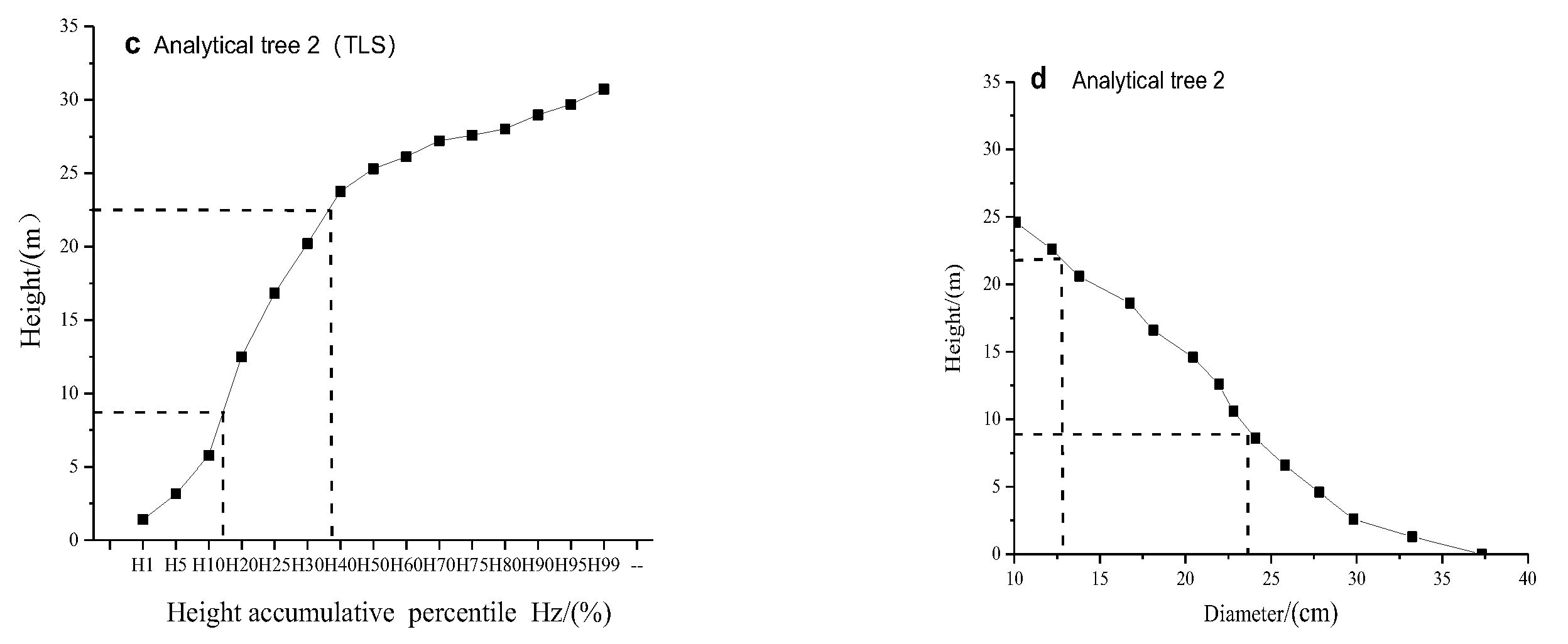
Data from the stem analysis were used to draw the taper curves, as shown in Figure 1b,d. Tree heights of 10 to 20 m represent the inflection points of the tree trunk. The point cloud data for these two trees were also drawn, as shown in Figure 1a,c. Hz% clearly increases with increasing height and reaches approximately 10 m of the tree height at 25%, which appears to be an inflection point; then, Hz% reaches approximately 20 m of the tree height at value of 50%, which appears to be another inflection point and is followed by a gentle increasing trend for Hz%.
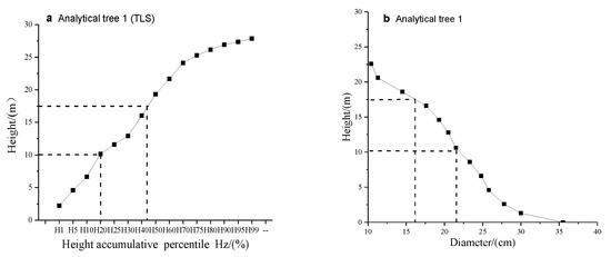

Figure 1.
Comparative analysis of the height cumulative percentile and analytical tree stem curve. (a,c) Height cumulative percentage (Hz%) versus height; (b,d) Analytical wood stem curve.
3.2. Features Extracted from the Point Cloud Data in Three Periods
This research extracted the tree structure parameters (DBH and tree height) and hierarchical features (Hz% and Hmean) and counted the volume of each standing tree in all three periods. A summary of the stumpage features is shown in Table 1. The average DBH of a single tree increased significantly, and the average annual growth was stable at 0.3 cm. The standard deviation of DBH growth was large at 5.95 in 2014, 6.49 in 2018, and 7.66 in 2019. The tree height and volume also increased annually. The average heights of H75, H55, and H25, which refer to the spatial distribution of tree trunks from top to bottom, decreased annually in accordance with the law of tree growth.

Table 1.
Summary of features of a single tree in the three periods.
3.3. Tree Volume Modeling Results
A Pearson correlation analysis was conducted on individual trees. According to the analysis results of the three periods, the DBH has the highest correlation with the tree volume, followed by the tree height, which conforms to the rule regarding the three elements of volume. Among the correlations between the hierarchical features and the tree volume, the highest correlation parameter in 2014 was H25, and then H50; the highest correlation parameter in 2018 was H25, and then H50; and the highest correlation parameter in 2019 was H80, and then H75.
Thus, the volume model was established by using the hierarchical features DBH and tree height as variables. The model results are shown in Table 2. Among them, the binary volume Serial No. 1 models are used as reference models and have the highest R2 values (0.974, 0.974, and 0.919, respectively), and H and DBH are variables. The Serial No. 2 models are also binary linear models with H25 and DBH as variables, and their R2 values are 0.951, 0.957 and 0.901. Table 2 shows that the models with hierarchical features (H50, H80, and H75) have slightly lower R2 values; however, these models seem to be better for predicting the volume, thus, revealing the efficacy of Hz%. In contrast, H25 is the first inflection point along the trunk.
Table 2.
Results of the volume model for individual trees.
The Serial No. 2 models are used to predict the individual tree volume, and the scatterplot of the predicted value of the model and the volume of individual tree in three periods were drawn. After verification, no significant difference was observed between the predicted volume and the volume extracted from the point cloud. Therefore, the volume model with hierarchical parameters can be used as the volume model for each period.
Then, the volume was counted for each DBH grade in each period, and the results are shown in Table 3. At the same time, the linear relationship of the volume changes in the DBH grades between the modeled values and the values extracted from the point cloud was established and determined to have an intercept of −0.081, a slope of 1.14, and an R2 of 0.98.
Table 3.
Volume variations in diameter at breast height (DBH) grades from 2014 to 2019.
3.4. Dynamic Analysis of the Tree Structure from Features
3.4.1. Individual Tree Changes and the Growth Rate
Table 4 displays the individual changes in growth rates of the tree height, DBH, and tree volume in the three phases. Since the investigated periods spanned four years and one year, the growth rates are distinguished as four-year and one-year rates. The average growth rates among the three phases are as follows: tree height average growth rate: 0.36–0.39 m; DBH average growth rate of 0.34−0.38 cm; and volume average growth rate of 0.02–0.03 m3. Among these rates, the average growth rate of the tree height is greater than the average growth rate in the four-year period 2014–2018. Moreover, the volume growth rates in all three periods are relatively average.
Table 4.
Growth rates of the features for individual trees in the three periods.
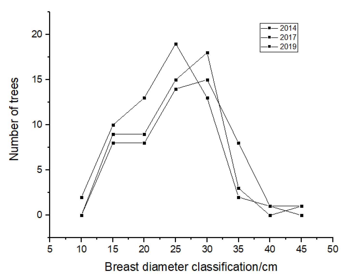
The variations in the diameter grades of the sample plot during the three periods are shown in Figure 2. The diameter step was 5 cm, and the initial diameter class was set to 5 cm. As the number of trees was counted by diameter class, the peak of the diameter distribution curve shifted from 25 cm in 2014 to 30 cm in 2018. Among the diameter classes, the shifted numbers of the 20 and 25 cm diameter classes were relatively high.
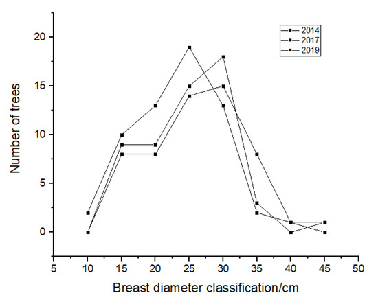
Figure 2.
Diameter grade distribution curves for 2014, 2018, and 2019.
3.4.2. Height Cumulative Percentage Analysis
The study calculates the change rate of height cumulative percentage of adjacent tree high, and the interval was 5%. For instance, the change rate from H10 to H15 is H15 minus H10 divided by H10. As shown in Table 5 the maximum change value of the change rate in the three periods are , which means that in the range of H20-H25-H35, the Hz change amplitude was the largest. Therefore, H25 is regarded as the mutation point of Hz change. These results indicate that the hierarchical features can reflect the change in the stem shape, and these features appear regularly within all five years. The height cumulative percentages of 25% for the Chinese tulip (L. chinense) tree is the inflection points for standing trees. As evidenced, the cumulative height percentage of the point cloud can reflect the change in the stem shape.
Table 5.
The change rate of Hz in three periods.
4. Discussion
First, laser scanning technology provides data with high density point cloud that can be used to extract related geometric and statistical parameters for individual trees. This study focuses on point cloud data obtained by TLS. After splicing, denoising, and normalization, the point cloud data have a relatively uniform point distribution regardless of the type of equipment. Photogrammetry and ALS technology can also achieve the same data distribution [13]. Therefore, whether vertical hierarchical parameters can be used as fusion features for multisource point cloud data is worthy of further discussion.
Second, in this paper, we studied the potential of TLS for estimating the volume of L. chinense in the study area by using point cloud hierarchical and statistical parameters. These parameters changed with the growth characteristics, namely, the tree height and canopy diameter. Through the analysis of the correlation between these parameters and volume, we concluded that the H50 and H25 were mostly correlated with volume. At the same time, the model based on these parameters had high accuracy and can be used for dynamic analysis (Table 3).
Third, the height of each quantile can be calculated analogously in a sample canopy profile of the ground [14]. The TLS data have dense point clouds under the canopy and can obtain structures with precision. This research defined the ground vertical characteristic parameter Hz%. This parameter extends the measurements of standing tree point clouds and extracts the characteristics reflecting the tree height and canopy from the vertical distribution features of point clouds. Whether this feature can reveal the trunk shape or not and whether Hz% is related to the planting density and species characteristics or not are worthy of further discussion. Hz% could also be discussed as a new taper parameter that can be obtained by laser scanning technology.
5. Conclusions
The significant outcome of the study is that our approach defined the ground vertical characteristic parameter Hz%, which is used to express the cumulative height of the first m points (from the bottom up to the first point) divided by all heights equal to Z% n points, with the first m point heights representing the Z% of the point cloud. This parameter extends the measurements of standing tree point clouds and extracts the characteristics reflecting the tree height and upper-diameter from the vertical distribution features of point clouds. This paper proposed that the corresponding model could be chosen according to the actual needs of the investigation based on the species and the scanning condition. The structure of standing tree could be derived from point cloud data, and a dynamic analysis could be performed through modeling.
Author Contributions
Y.S. conceived and designed the experiment. X.L., X.W. and J.J. performed the experiments and analyzed the data. X.L., Y.G. and Y.Z. wrote the manuscript. All authors have read and agreed to the published version of the manuscript.
Funding
This study was funded by the Natural Science Foundation of Jiangsu Province (BK20191388), Jiangsu Provincial Postgraduate Research and Practice Innovation Program (KYCX20_0900), Priority Academic Program Development of Jiangsu Higher Education Institutions (PAPD) and the China Postdoctoral Science Foundation (2016M601822).
Conflicts of Interest
The authors declare that they have no conflict of interest.
References
- Hilker, T.; Wulder, M.A.; Coops, N.C. Update of forest inventory data with Lidar and high spatial resolution satellite imagery. Can. J. Remote Sens. 2014, 34, 5–12. [Google Scholar] [CrossRef]
- Simonse, M.; Aschoff, T.; Spiecker, H.; Michael, T. Automatic determination of forest inventory parameters using terrestrial laser scanning. In Proceedings of the Scandlaser Scientific Workshop on Airborne Laser Scanning of Forests; Sveriges Lantbruksuniversitet: Umeå, Sweden; 2003. (In Germany)
- Pfeifer, N. Automatic reconstruction of single trees from terrestrial laser scanner data. Int. Arch. Photogramm. Rem. Sens. 2004, 35, 114–119. [Google Scholar]
- Liang, X.L.; Kankare, V.; Hyyppä, J.; Wang, Y.S.; Kukko, A.; Haggrén, H.; Yu, X.W.; Kaartinen, H.; Jaakkola, A.; Guan, F.Y.; et al. Vastaranta, M. Terrestrial laser scanning in forest inventories. ISPRS J. Photogramm. Remote Sens. 2016, 115, 63–77. [Google Scholar] [CrossRef]
- Erikson, M.; Karin, V. Finding tree-stems in laser range images of young mixed stands to perform selective cleaning. In Proceedings of the Scandlaser Scientific Workshop on Airborne Laser Scanning of Forest; Sveriges Lantbruksuniversitet: Umeå, Sweden, 2003; pp. 244–250. (In Germany). [Google Scholar]
- Thies, M.; Spiecker, H. Evaluation and future Prospects of terrestrial laser scanning for standardized forest inventories. In Proceedings of the ISPRS working group VIII/2 Laser-Scanners for Forest and Landscape Assessment, Freiburg, Germany, 3–6 October 2004. (In Germany). [Google Scholar]
- Sun, Y.; Liang, X.L.; Liang, Z.Y.; Welham, C.; Li, W.Z. Deriving merchantable volume in poplar through a localized tapering function from non-destructive terrestrial laser scanning. Forests 2016, 7, 87–97. [Google Scholar] [CrossRef]
- Seidel, D.; Ehbrecht, M.; Puettmann, K. Assessing different components of three-dimensional forest structure with single-scan terrestrial laser scanning: A case study. For. Ecol. Manag. 2016, 381, 196–208. [Google Scholar] [CrossRef]
- Næsset, E. Predicting forest stand characteristics with airborne scanning laser using a practical two-stage procedure and field data. Remote Sens. Environ. 2002, 80, 88–99. [Google Scholar] [CrossRef]
- Grilli, E.; Menna, F.; Remondino, F. A review of point clouds segmentation and classification algorithms. In Proceedings of the ISPRS-International Archives of the Photogrammetry, Remote Sensing and Spatial Information Sciences, Nafplio, Greece, 1–3 March 2017; pp. 339–344. [Google Scholar]
- Meng, X.Y. Forest Measuration; China Forestry Publishing House: Beijing, China, 2006. [Google Scholar]
- Li, Y.M.; Guo, Q.H.; Su, Y.J.; Tao, S.L.; Zhao, K.G.; Xu, G.C. Retrieving the gap fraction, element clumping index, and leaf area index of individual trees using single-scan data from a terrestrial laser scanner. ISPRS J. Photogramm. Remote Sens. 2017, 130, 308–316. [Google Scholar] [CrossRef]
- Srinivasans, S.; Popescu, S.C.; Eriksson, M.; Sheridan, R.D.; Ku, N.W. Multi-temporal terrestrial laser scanning for modeling tree biomass change. For. Ecol. Manag. 2014, 318, 304–317. [Google Scholar] [CrossRef]
- Maguya, A.; Tegel, K.; Junttila, V.; Tuomo, K.; Markus, K.; Janice, B.; Vesa, L.; Blanca, S. Moving voxel method for estimating canopy base height from airborne laser scanner data. Remote Sens. 2015, 7, 8950–8972. [Google Scholar] [CrossRef]

Publisher’s Note: MDPI stays neutral with regard to jurisdictional claims in published maps and institutional affiliations. |
© 2020 by the authors. Licensee MDPI, Basel, Switzerland. This article is an open access article distributed under the terms and conditions of the Creative Commons Attribution (CC BY) license (https://creativecommons.org/licenses/by/4.0/).