Transport Cost Estimation Model of the Agroforestry Biomass in a Small-Scale Energy Chain ^†

Abstract

The delivery of biomass products from the production place to the point of final use is of fundamental importance within the constitution of energy chains based on biomass use as renewable energy source. In fact, transport can be one of the most economically expensive operations of the entire biomass energy production process. In this work, a geographic identification, through remote sensing and photo-interpretation, of the different biomass sources was used to estimate the potential available biomass for energy in a small-scale supply chain. The economic sustainability of transport costs was calculated for different types of biomass sources available close to a biomass power plant of a small-scale energy supply chain, in central Italy. The proposed analysis allows us to highlight and visualize on the map the areas of the territory characterized by greater economic sustainability in terms of lower transport costs of residual agroforestry biomass from the collection point to the final point identified with the biomass power plant. The higher transport cost was around € 40 Mg⁻¹, compared to the lowest of € 12 Mg⁻¹.

1. Introduction

The interest in the use of renewable energies and bioenergy is always increasing on a planetary level, especially about the decisive role that they can play in terms of contrasting the climate changes taking place in substitution of fossil fuels considered the most responsible of greenhouse gas emissions [1,2,3]. There are different types of biomass that can be used for energy purposes and numerous technologies have been developed for their conversion into different forms of energy (thermal, electrical, liquid fuels and biogas). Each energy form corresponds to equally diversified energy chains. The logistical organization of these supply chains represents one of the priority aspects on which most of the impacts (economic, occupational, environmental, etc.) depend, and of the real convenience to the production of primary energy from agroforestry biomass. It is therefore essential to make the entire production process of energy transformation sustainable, from the collection and transport of the raw material, to its final transformation, by applying models that can improve the efficiency of production processes and optimize production costs for each type of biomass available [4,5,6]. Among the cost items of the energy supply chain, transport certainly represents a key element that heavily affects the economic and environmental sustainability of the energy supply and production chain [7]. In this sense, the short energy chain and the priority enhancement of the biomasses spread throughout the territory in the vicinity of the transformation plant represent the basis for sustainable development of bioenergy [8].

The present work examines a small territorial basin of a small local energy supply chain [9], where different sources of agroforestry biomass are available. A geographic model was built on the area to evaluate the economics of the logistics of transport of agroforestry biomass, taking into consideration both technical and economic data (transport times and costs, biomass loading and unloading), and data relating to the territory, such as type of biomass and its location, qualitative and quantitative availability, viability and possible routes with respect to the transformation point.

2. Materials and Methods

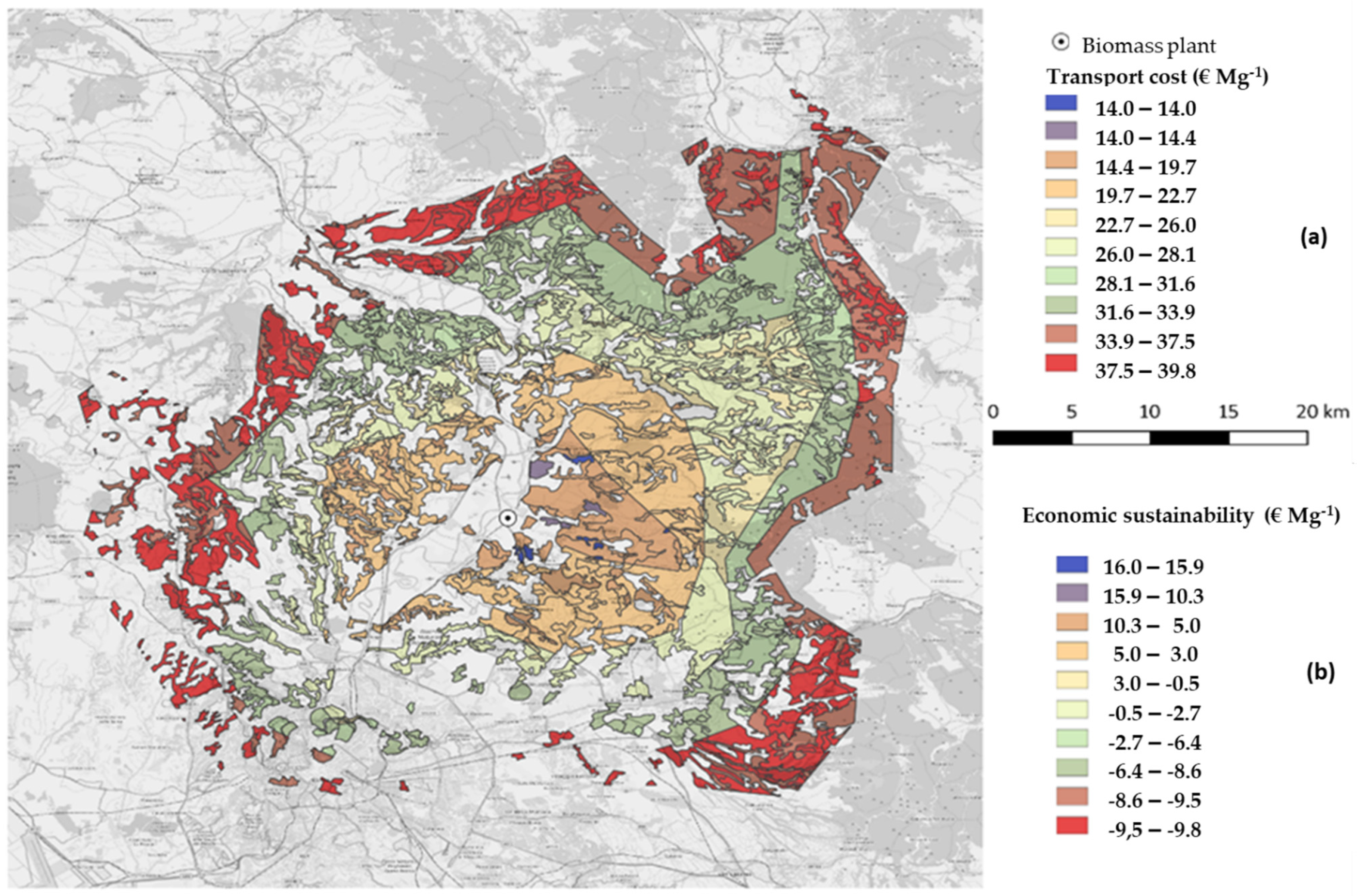
2.1. Study Area and Biomass Power Plant

The study area refers to a small-scale supply chain located in the north-east of Rome, with a biomass power plant installed within the CREA farm-Research Center for engineering and agri-food processing of Monterotondo, Italy (42°6′2.63″ N; 12°37′37.36″ E). The boundaries of the potential wood biomass supply area were based on the travel time of the trucks from any spatial point located no more than 60 min from the biomass plant, selecting the road with the shortest travel time, excluding highways [9]. For this reason, the conformation of the study area is irregular and depends on the spatial arrangement of the road network, the types of roads and the speed limits. Five areas consisting of irregular isochronous rings were identified. The first ring, the most external, is the one with a travel time varying from 60 to 50 min; the second from 50 to 40, the third from 40 to 30, the fourth from 30 to 20 and finally the fifth ring, the closest to the biomass plant, from 20 to 0 min. The isochronous rings have been calculated by applying the software package R osrm (OpenStreetMap-Based Routing Service) version 3.2.0 [10]. The furthest point of the outer boundary of the area from the plant was at a linear distance of about 35 km, while the closest was about 16 km. The total area examined was 2276 km², increasingly distributed from the fifth to the first isochronous ring.

The proposed model was built with reference to the specific point of energy transformation, represented by the 350 kW biomass power plant used for heating the buildings of the Research Center. The plant is also set up for micro-cogeneration, using a steam turbine to produce approximately 40 kWh of electricity. For the heating of buildings alone, the potential biomass that can be consumed annually is about 290.1 Mg. By also activating the cogeneration option, the annual consumption of biomass would rise to approximately 811.5 Mg.

2.2. Biomass Estimation

The residual biomass, present in the observed area, divided by type, was estimated by interpreting satellite images taken from the Google Earth software [9]. The quantitative estimation was made by applying judgment coefficients of photointerpretation experts. Out of a total of 139 observations, eight sampling populations were defined, each of which was independently sampled. Eight types of biomass classes have been identified, on which the transport cost assessment model has been applied:

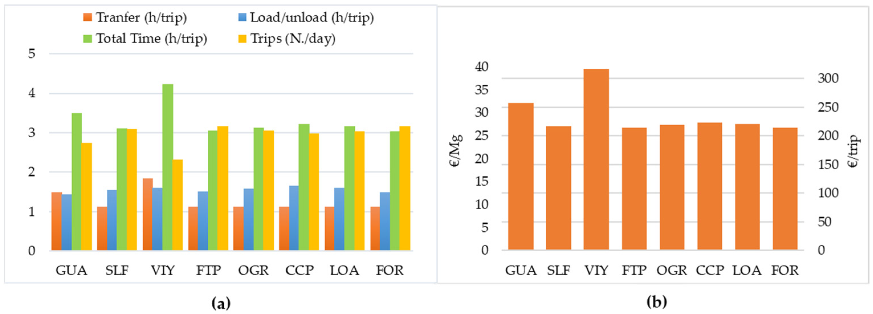
• green urban area (GUA); considering an average density of 80 trees ha⁻¹, intervention cycles repeated every 8 years, with an estimated production of 16–32 Mg ha⁻¹;
• sports and recreational facilities (SLF); like GUA, but considering a lower average density, 50 trees ha⁻¹, with an average production of 10.4–20.0 Mg ha⁻¹, and with pruning every 8 years;
• vineyards (VIY); pruning biomass of about 0.7–1.0 kg tree⁻¹; density of 3000–4000 trees ha⁻¹; with annual pruning;
• fruit trees and berry plantations (FBP); plantation density about 400–500 trees ha⁻¹; pruning production estimated at 5.0–7.0 kg tree⁻¹;
• olive grove (OGR); planting density about 180–300 trees ha⁻¹, production of 20.0–27.0 kg tree⁻¹, with pruning every two years;
• complex cultivation models (CCP); considering 130–260 trees ha⁻¹, biomass production of 2.0–4.0 Mg ha⁻¹, pruning every two years;
• land mainly occupied by agriculture (LOA); considering a density of about 400–500 trees ha⁻¹, biomass production about 2.0–3.5 Mg ha⁻¹, pruning every year;
• forests (FOR); considering mainly broad-leaved woods, coppices with residual biomass production of 19–26 Mg ha⁻¹, in 25-year cycles.

Based on the coverage of the tree canopy observed on the territorial map, for each of the eight classes, four decreasing levels of biomass production (in Mg ha⁻¹ y⁻¹) have been attributed (

Table 1. Biomass production levels (L) considered for the calculation of biomass available for each typological class (in Mg ha⁻¹ y⁻¹).

Typology	L3	L2	L1	L0
Green Urban Areas (GUA)	4.00	3.00	2.00	0.00
2. Sport and Leisure Facilities (SLF)	2.50	1.90	1.30	0.00
3. Vineyards (VIY)	3.00	2.55	2.10	0.00
4. Fruit Trees and berry Plantation (FTP)	3.50	2.75	2.00	0.00
5. Olive Groves (OGR)	4.00	2.90	1.80	0.00
6. Complex Cultivation Patterns (CCP)	2.00	1.50	1.00	0.00
7. Land principally Occupied by Agriculture (LOA)	3.50	2.75	2.00	0.00
8. Forest class (FOR)	1.05	0.90	0.75	0.00

). In this way, a set of data was built referring to each single area of the map, identifying the type, the overall surface, the percentage of the surface referred to the different biomass level potentially available and the belonging to a specific isochronous ring.

2.3. Transport Cost Evaluation Model

The analysis of the economic sustainability of the biomass recovery and transport was based on the evaluation of the costs of the transport operation, including the transfer of the biomass from pre-processing sites to the main processing plant and the loading and unloading operations. The hypothesis adopted is that farmers supply pruning biomass for free to avoid incurring in the fees charged for the disposal of this material in landfills. Both the farmer and the power plant manager benefit from the deal: the former does not pay for the disposal; the latter does not pay for the raw material recovered. In the case study, the pruning biomass is staked by the farmer and directly available for transport. It is assumed that an unloaded truck departs from the power plant and arrives at the biomass loading site, where a forest loader loads the pruning biomass.

Once the loading operation is complete, the truck makes the journey and unloads the biomass near the biomass plant. The truck carries out the subsequent operations until the completion of the scheduled working time (8 working hours per day). It was assumed that this operation was carried out using a single truck with a total load capacity of 26 m³, corresponding to about 8 Mg. A forestry loader equipped with a grapple to carry out the loading/unloading of biomass must be transferred daily to the workplace and brought back via a dedicated truck. The hourly costs of the machines calculated with analytical methodology [11], and the main economic and technical elements considered, are shown in

Table 2. Principal elements considered for the machines hourly cost and manpower.

	Truck for Biomass Transport	Truck for Loader Transport	Forest Loader
Purchase price (€)	110,000	95,000	80,000
Salvage value (€)	7559	6528	8590
Life time (years)	12	12	10
Total time (h)	14,400	14,400	8000
Engine Power (kW)	309	280	88
Interest rate (%)	4.0	4.0	4.0
Fuel consumption (l h−1)	25.49	23.10	9.44
Fuel price (€ l−1)	1.50	1.50	1.10
Driver cost (€ h−1)	21.00	21.00	15.00
Machine cost (€ h−1)	71.00	64.00	35.00
Total operating cost (€ h−1)	92.00	85.00	50.00

.

The formula used to determine the unitary transport cost (Equation (1)), including the biomass loading, transport and unloading cost and the daily forest loader transfer cost, is the following:

$$CTB=\frac{\left[\left(Ttr\times Ctr)+(Tlu\times Clo\right)+\left(tcl\times Ctl\right)\right]}{bl},$$

(1)

where:

CTB	biomass transport cost per Mg (€ Mg−1);
Ttr	roundtrip travel time, obtained doubling the return travel time of the loaded truck (h);
Tlu	time required for loading and unloading operations (h);
Ctr	hourly cost of the truck (€ h−1);
Clo	hourly cost of the loader (€ h−1);
tcl	transferring coefficient;
Ctl	hourly cost of the truck that transfer the loader to destination and return (€ h−1);
bl	average biomass load considered per travel (t).

To consider the influence of the different types and quantity of biomass on the load operation, multiplier coefficients of the load time were used. Other correction coefficients have been applied to consider the displacements required to complete a load. The impact of the loader transfer time on the total travel time was estimated considering a loader transfer coefficient to calculate the additional time (

Table 3. Coefficients used for the calculation of final travel time (lc, loader coefficient; yc, yield coefficient; tc, loader transfer coefficient).

Typology	Coefficients
	lc	yc	tc
GUA	1.00	0.20	0.37
SLF	1.05	0.29	0.34
VIY	1.15	0.21	0.43
FTP	1.05	0.21	0.33
OGR	1.10	0.23	0.34
CCP	1.10	0.30	0.35
LOA	1.15	0.21	0.34
FOR	1.00	0.27	0.30

).

In order to evaluate the economic sustainability of the recovery and transport of biomass spread over the territory of the small-energy chain, it was necessary to consider that the biomass unloaded at the plant had to be chipped before use. A positive assessment on economic sustainability was based on the positive difference between the average value of the wood chips and the cost incurred for transport and chipping. The chipping operation was performed using a company forest chipper. The average cost of this operation was estimated in € 15 Mg⁻¹. The value of the woodchip was quoted at around € 45 Mg⁻¹.

3. Results and Discussion

In Figure 1, the average times consumed (Figure 1a) and relative average costs (Figure 1b) of the load, transport and unload operations of the residual biomass for each class are reported. The highest total time is request for the VIY class with 4.23 h trip⁻¹, while the shortest time is recorded for the FOR class, with 3.04 h trip⁻¹. The other biomass classes record intermediate times between 3.05 and 3.50 h trip⁻¹. The load/unload time is highest in CCP class with 1.65 h, followed by LOA and VIY with 1.61 h, while GUA requires the lowest time of 1.44 h. The trend in average costs per trip reflects that of the times with the highest value of € 316.31 trip⁻¹ for VIY, corresponding to € 39.54 Mg⁻¹, and the lowest value of € 213.84 trip⁻¹ for FOR, that is € 26.73 Mg⁻¹.

It should be specified that, with regard to the VIY class, it is not abundant in the area observed, so it is not to be considered a representative data for the class examined. For the other classes, instead, there is a greater homogeneity of results for the classes FTP, OGR, CCP and LOA. The cost increases by proceeding from the 5th isochronous ring (journey time 0–20 min) to the 1st (50–60 min). This is valid for all classes even if in a different way. The average costs varying from minimum of about € 14 Mg⁻¹ in the area of the 5th ring, to maximum of about € 39.80 Mg⁻¹ in the 1th ring. Economic sustainability is inversely proportional to the costs incurred. Figure 2 shows the territorial map in which the transport costs are associated with the location of the area to which they refer. From this map it is possible to check the transport cost (Figure 2a) in relation to the distance from the plant of the biomass to recover. The economic sustainability conditions (Figure 2b) occur at positive values, i.e., in the areas ranging from yellow to blue (proximity of the biomass plant).

Compared to the total area and the related potential biomass available, only that relating to the 4th and 5th isochronous ring presents conditions of economic sustainability, showing a positive difference between the woodchip value and calculated costs.

On a total area of 2276 km², about 57% of this, equal to 130 kha, was considered in the model. The annual residual biomass potentially available was about 134 Gg distributed on the territory observed. Much of the biomass available was classified as agricultural area (LOA) for about 34.4%, followed by olive groves with 33% and forest area with 23.8%. The remaining 8.8% is mainly divided between associated crops and orchards. Of this total biomass available, only 24% falls within the area of the economic sustainability (5 and 4 isochronous rings) for a quantity of about 32 Gg, 62% of which represented by olive grove pruning residues. For the case study, only a small percentage of this available biomass can be used in the biomass plant, whose annual consumption in cogeneration system does not exceed 1 Gg of woodchip.

The economic evaluation model is applied to the different types of biomass available, considering the various difficulties related to the quality of biomass residues and the influence this generates in the calculation of recovery and transport costs [12,13]. The model, as expected, returns highest transport costs in correlation to greatest distances to travel. For the examined small-scale energy chain, the economic sustainability for the supply of biomass to feed the plant is verified when the travel distance was not exceeding 20 km, with a travel time from the place where the biomass is loaded to the plant, no more than 35 min. At equal distance from the power plant, the pruning residues of orchards and forest biomass are slightly more advantageous than the other classes, while the pruning of vineyards, being represented only within the most distant isochronous ring, are always uneconomical.

4. Conclusions

The study carried out was aimed at implementing a geographic evaluation model capable of providing a mapping of the costs of transporting biomass (including loading and unloading) from production sites to processing sites. By mapping the cost of biomass transport, it is possible to guide the choices in relation to the size of the energy transformation plants to be considered also in a project to enhance the local resources available. The short supply chain, in fact, currently represents a model to be encouraged and applied in farms that want to make a qualitative leap towards a bioenergy company. The start of a virtuous process of mutual benefit between the farmers of a territory and the bioenergy company, results in a recovery of the residual biomass, otherwise destined for landfill or burned in the field, to enhance it in the production of energy. In this way, environmental impacts are also reduced thanks to a more controlled combustion process in small biomass plants.

References

1. Nishiguchi, S.; Tabata, T. Assessment of social, economic, and environmental aspects of woody biomass energy utilization: Direct burning and wood pellets. Renew. Sustain. Energy Rev. 2016, 57, 1279–1286. [Google Scholar] [CrossRef]
2. Tziolas, E.; Manos, B.; Bournaris, T. Planning of agro-energy districts for optimum farm income and biomass energy from crops residues. Oper. Res. 2017, 17, 535–546. [Google Scholar] [CrossRef]
3. Martín-Lara, M.A.; Ronda, A.; Zamora, M.C.; Calero, M. Torrefaction of olive tree pruning: Effect of operating conditions on solid product properties. Fuel 2017, 202, 109–117. [Google Scholar] [CrossRef]
4. Cambero, C.; Sowlati, T.; Marinescu, M.; Röser, D. Strategic optimization of forest residues to bioenergy and biofuel supply chain. Int. J. Energy Res. 2015, 39, 439–452. [Google Scholar] [CrossRef]
5. Paulo, H.; Azcue, X.; Barbosa, A.P.; Relvas, S. Supply chain optimization of residual forestry biomass for bioenergy production: The case study of Portugal. Biomass Bioenergy 2015, 83, 245–256. [Google Scholar] [CrossRef]
6. Sierk de Jong, S.; Hoefnagels, R.; Wetterlund, E.; Pettersson, K.; Faaij, A.; Junginger, M. Cost optimization of biofuel production—The impact of scale, integration, transport and supply chain configurations. Appl. Energy 2017, 195, 1055–1070. [Google Scholar] [CrossRef]
7. Zhang, Y.; Qinb, C.; Liuc, Y. Effects of population density of a village and town system on the transportation cost for a biomass combined heat and power plant. J. Environ. Manag. 2018, 223, 444–451. [Google Scholar] [CrossRef] [PubMed]
8. Verani, S.; Sperandio, G.; Picchio, R.; Marchi, E.; Costa, C. Sustainability Assessment of a Self-Consumption Wood-Energy Chain on Small Scale for Heat Generation in Central Italy. Energies 2015, 8, 5182–5197. [Google Scholar] [CrossRef]
9. Bascietto, M.; Sperandio, G.; Bajocco, S. Efficient Estimation of Biomass from Residual Agroforestry. ISPRS Int. J. Geo-Inf. 2020, 9, 21. [Google Scholar] [CrossRef]
10. Luxen, D.; Vetter, C. Real-time routing with OpenStreetMap data. In Proceedings of the 19th ACM SIGSPATIAL International Conference on Advances in Geographic Information Systems, Chicago, IL, USA, 1–4 November 2011; ACM: New York, NY, USA, 2011; pp. 513–516. [Google Scholar]
11. Miyata, E.S. Determining Fixed and Operating Costs of Logging Equipment; General Technical Report NC-55; Department of Agriculture, Forest Service, North Central Forest Experiment Station: St. Paul, MN, USA, 1980. [Google Scholar]
12. Paolotti, L.; Martino, G.; Marchini, A.; Boggia, A. Economic and environmental assessment of agro-energy wood biomass supply chains. Biomass Bioenergy 2017, 97, 172–185. [Google Scholar] [CrossRef]
13. Zahraee, S.M.; Shiwakoti, N.; Stasinopoulos, P. Biomass supply chain environmental and socio-economic analysis: 40-Years comprehensive review of methods, decision issues, sustainability challenges, and the way forward. Biomass Bioenergy 2020, 142, 105777. [Google Scholar] [CrossRef]
Figure 1. Time consumption (a) and costs (b) for the recovery and transport of residual biomass per each class.
Environsciproc 03 00022 g001
Figure 2. Territorial Map of the biomass transport cost (a) and economic sustainability of the operation (b) according to typological classes and isochronous rings.
Environsciproc 03 00022 g002