FORTLS: An R Package for Processing TLS Data and Estimating Stand Variables in Forest Inventories ^†

Abstract

Terrestrial Laser Scanning (TLS) enables rapid, automatic, and detailed 3D representation of surfaces with an easily handled scanner device. TLS, therefore, shows great potential for use in Forest Inventories (FIs). However, the lack of well-established algorithms for TLS data processing hampers operational use of the scanner for FI purposes. Here, we present FORTLS, which is an R package specifically developed to automate TLS point cloud data processing for forestry purposes. The FORTLS package enables (i) detection of trees and estimation of their diameter at breast height (dbh), (ii) estimation of some stand variables (e.g., density, basal area, mean, and dominant height), (iii) computation of metrics related to important tree attributes estimated in FIs at stand level, and (iv) optimization of plot design for combining TLS data and field measured data. FORTLS can be used with single-scan TLS data, thus, improving data acquisition and shortening the processing time as well as increasing sample size in a cost-efficient manner. The package also includes several features for correcting occlusion problems in order to produce improved estimates of stand variables. These features of the FORTLS package will enable the operational use of TLS in FIs, in combination with inference techniques derived from model-based and model-assisted approaches.

1. Introduction

Information about forest resources is essential for sustainable forest management and development of forest policies. In this regard, forest inventories (FIs) are used as the main approach for estimating and monitoring the state and evolution of the main variables of interest. FIs have improved since they were first introduced, as a result of the continuous appearance of new technologies, such as Terrestrial Laser Scanning (TLS), considered of great potential value for enhancing FIs [1,2]. However, TLS has not yet been adopted in FIs for several reasons [3]. However, many studies agree that affordability is the main key challenge to overcome, emphasizing that automation of the point cloud processing with attainable and easy-to-use software able to extract information related to important forest attributes is essential [1,2,3,4,5].

Since TLS data sets comprise millions of points, sophisticated methods for automatic processing are necessary. In this respect, many algorithms with a high level of automation that are able to extract tree attributes (diameter at breast height, dbh, height, volume, etc.) have been developed in the last few decades [6]. Some of these algorithms have also been included in software applications, e.g., SimpleTree [7], 3D Forest [8], and AutoStem^TM [9]. However, there are some drawbacks to using these applications in FIs: (i) single-tree instead of stand-level approaches (SimpleTree), (ii) semi-automatic processing (3D Forest), and (iii) commerciality (not suitable for all users) (AutoStem^TM).

Here, we present FORTLS, an R package developed with the objective of automating TLS point cloud data processing and estimating variables for forestry purposes. FORTLS can be used with single-scan TLS data and enables (i) detection of trees and estimation of dbh, (ii) estimation of some stand variables, such as density (N, trees ha⁻¹), basal area (G, m² ha⁻¹), and mean and dominant height, defined as the mean height of the 100 largest trees ha⁻¹ (h_m and H₀ respectively), (iii) computation of metrics related to important tree attributes estimated in FIs at stand level, and (iv) optimization of plot design for combining TLS data and field measured data. These features of the FORTLS package will enable the operational use of TLS in FIs in combination with model-based or model-assisted inference approaches.

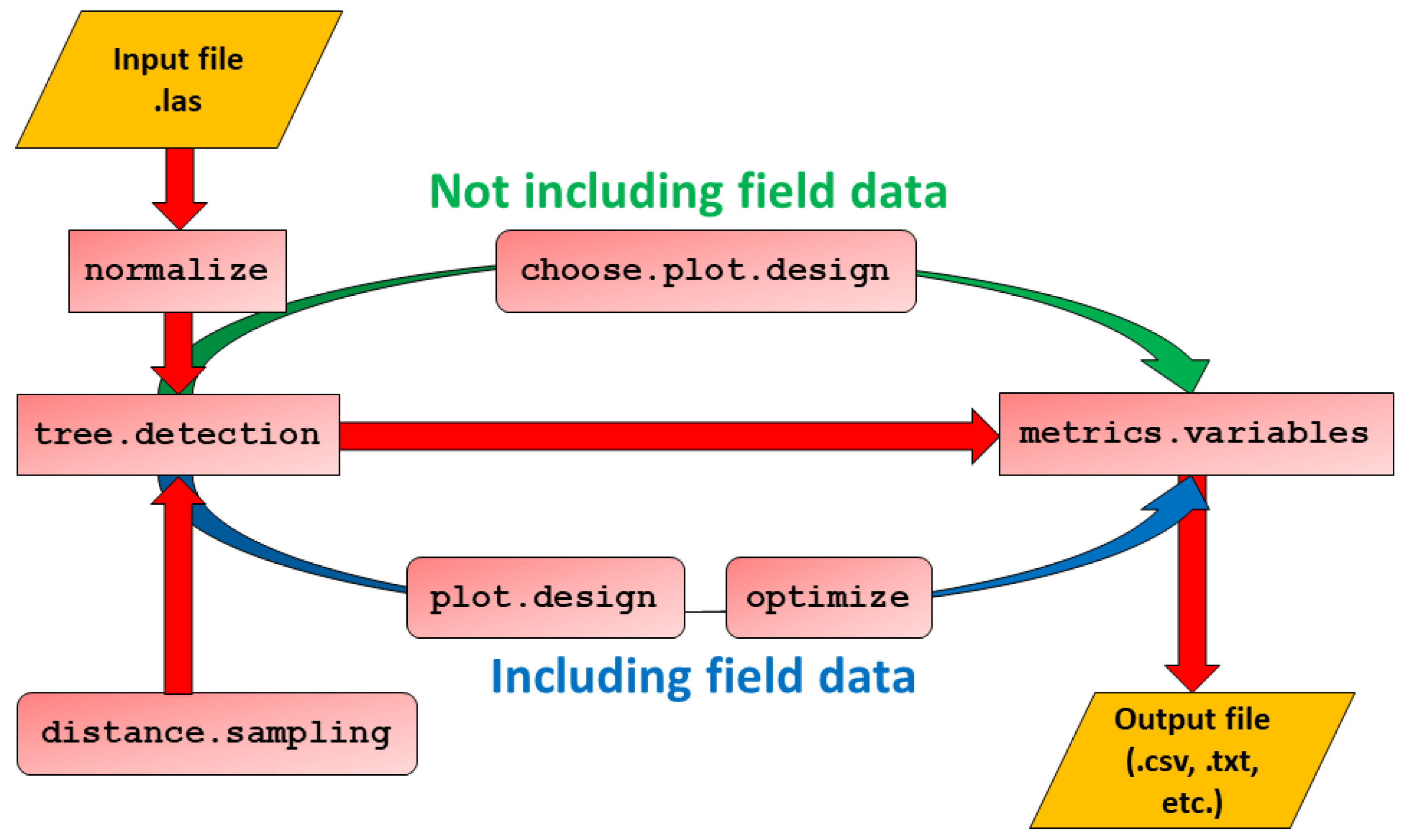
2. Materials and Methods

The steps involved in the TLS data processing algorithms are described in the following sections.

2.1. Detection of Trees and Estimation of dbh

This first algorithm detects trees and estimates their dbh, which is the basis for further computations. This is done by the normalize function (Figure 1), which obtains coordinates relative to the plot centre and the digital terrain model. This function also applies the point cropping process as a criterion for reducing point density homogeneously in space and proportional to object size [10]. The output generated is then used as input for the tree.detection function, which detects as many trees as possible from point clouds in the TLS scans. In addition, for every tree detected, the function calculates the coordinates of the section centre, estimates dbh, and classifies it as fully visible or partially occluded. Finally, this function obtains the number of points corresponding to 1.3-m height sections of trees (i.e., the dbh) for original and reduced point clouds (by applying a point cropping process) as well as their estimations.

2.2. Computation of Variables and Metrics Related to Attributes Estimated in FIs at the Stand Level

Once trees have been detected, the next application of FORTLS is to compute variables and metrics at plot level. For this purpose, the metrics.variables function produces a set of TLS-based variables and metrics related to forest attributes. These can be obtained for different plot designs (circular fixed area, k-tree, and angle-count) if specified in the arguments. This function also includes features for correcting occlusion problems generated in TLS point clouds. These features are based on correcting the shadowing effect [11] and gap probability attenuation with distance to TLS [12]. Apart from these features, others based on distance sampling methods can be applied with the distance.sampling function by implementing point transects methods with the trees detected [13]. This calculates the detection probability for every tree by fitting probability detection functions to the histogram of trees distribution, according to their distance from the plot centre. As in previous studies by the same authors [13], half normal and hazard rate probability functions without and with dbh as a covariate were used.

Before using the metrics.variables function, previous steps are recommended in order to select the most appropriate values for the radius, k-tree, and BAF (Basal Area Factor) in the function arguments. This can be done with or without field data.

2.2.1. Field Measurements Not Available

In this case, the choose.plot.design function can be used to plot empirical charts of N and G estimates as a function of the plot size (estimation-size charts) for different plot designs (circular fixed area, k-tree, and angle-count) through continuous size increments (radius, k, and BAF, respectively). These size-estimation charts represent the consistency in predicting the stand variables across different values of radius, k, and BAF. Size-estimation charts can be drawn for individual sample plots (including all plots together in the same charts) or for mean values (global mean computed for all the sample plots, or for group means if different strata are considered). Finally, different plot designs can be compared if specified in the arguments, producing one size-estimation chart per variable (N and G).

2.2.2. Field Measurements Available

When field measurements are available for the same positions of TLS single-scans, the plot.design and optimize functions can be used to assess the performance of TLS-based metrics and variables relative to field measurements. The plot.design function examines correlations (Pearson and Spearman) and the relative deviance between TLS-based estimates and field measurements, through plots with a continuous size increment. This is done for different plot designs and by default for the most common metrics and variables. However, other metrics/variables may be considered in the arguments. In a second step, those metrics and variables most closely correlated with the variables of interest are evaluated by the optimize function. This function generates heatmaps (one per plot design) in which correlations between TLS metrics-variables and estimations of variables based on field data can be evaluated for all variables and plot sizes.

3. Results

The outputs of the previously mentioned functions are reported below.

3.1. Detection of Trees and Estimation of Their dbh

The result of these applications is a list of the trees detected with the previously mentioned tree.detection function, which is a data frame object containing attributes for every tree detected (

Table 1. Data frame with detected trees and their estimated attributes.

id	file	Tree	x y	phi phi.left phi.right	dbh Horizontal.Distance	num.points num.points.est num.points.hom num.points.hom.est	partial.occlusion
numeric/ character	character (id.txt)	numeric (n)	numeric (m)	numeric (rad)	numeric (m)	numeric (n)	numeric (0–1)

id: identification assigned to a sample plot and which coincides with the file name. file: file name, consisting of the id and the respective extension (.txt, csv, etc.). tree: number assigned to every detected tree (1, 2, …, n). x: x coordinate of tree centre relative to plot centre. y: y coordinate of tree centre relative to plot centre. phi: azimuth of tree centre from plot centre. phi.left: azimuth corresponding to left border of tree section detected. phi.right: azimuth corresponding to right border of detected tree section. dbh: estimated diameter at breast height. horizontal.distance: horizontal distance from sample plot centre to tree centre. num.points: number of points corresponding to normal tree section (1.3 ± 0.05 m). num.points.est: estimated number of points corresponding to normal tree section (1.3 ± 0.05 m). num.points.hom: number of points corresponding to normal tree section (1.3 ± 0.05 m) after the point cropping process. num.points.est: estimated number of points corresponding to normal tree section (1.3 ± 0.05 m) after the point cropping process. partial.occlusion: tree fully visible (0) or partial occluded (1).

).

3.2. Computation of Variables and Metrics Related to Attributes Estimated in FIs at Stand Level

The output of the function metrics.variables is a list with three data frames, one per plot design (circular fixed area, k-tree, and angle-count plot), containing the following metrics and variables included in

Table 2. Structure of list containing metrics and variables.

	N	G	V	dbhm	dbh0	Number of Points Belonging to Normal Sections	Percentiles
fix.plot k.tree angle.count	N N.hn 1 N.hr 1 N.hn.cov1 N.hr.cov 1 N.sh 1 N.corr 2	G G.hn 1 G.hr 1 G.hn.cov 1 G.hr.cov 1 G.sh1 G.corr 2	V V.hn 1 V.hr 1 V.hn.cov 1 V.hr.cov 1 V.sh 1 V.corr 2	dbh.arit dbh.sqrt dbh.geom dbh.harm	dbh.dom.arit dbh.dom.sqrt dbh.dom.geom dbh.dom.harm	num.points num.points.est num.points.hom num.points.hom.est	P1, P5, P10, P20, P25, P30, P40, P50, P60, P70, P75, P80, P90, P95, P99

N: all N variables are direct estimates of N, estimated using trees detected in TLS data. They are computed without considering occlusion corrections (N) and by implementing distance sampling methodologies (N.hn, N.hr, N.hn.cov, N.hr.cov), shadowing effect (N.sh) and gap probability attenuation with distance from TLS (N.corr). G: all G variables are direct estimates of G, estimated using detected trees from TLS data. They are computed without considering occlusion corrections (G) and by implementing distance sampling methodologies (G.hn, G.hr, G.hn.cov, G.hr.cov), a shadowing effect (G.sh), and gap probability attenuation with distance from TLS (G.corr). V: all V variables are direct estimates of V, estimated using trees detected in TLS data. They are computed without considering occlusion corrections (V) and by implementing distance sampling methodologies (V.hn, V.hr, V.hn.cov, V.hr.cov), a shadowing effect (V.sh), and gap probability attenuation with distance from TLS (V.corr). dbh_m: estimated dbh mean for detected trees using arithmetic (dbh.arit), square (dbh.sqrt), geometric (dbh.geom), and harmonic means (dbh.harm). dbh₀: estimated dominant dbh mean (considering the 100 largest trees ha⁻¹) for trees detected using arithmetic (dbh.dom.arit), square (dbh.dom.sqrt), geometric (dbh.dom.geom), and harmonic means (dbh.dom.harm). Number of points belonging to normal sections: sum of points belonging to normal sections of all trees detected from the original point cloud (num.points) and reduced point cloud, reduced using a point cropping process (num.points.hom), and number of points estimated from the original point cloud (num.points.est) and reduced point cloud, reduced using the point cropping process (num.points.hom.est). Percentiles: percentile of z coordinate (m) relative to ground level. ¹ Variables are computed for the fix area and k-tree plots. ² Variables are computed for angle count plots.

:

3.2.1. Plot Design When Field Measurements Are Not Available

Figure 2 is an example of choose.plot.design output when no arguments are defined. In these graphical representations, it can be observed that estimations of N and G become approximately stable from a radius of 8 m (circular fixed area plot) and 10 trees (k-tree plot) and between 1 and 2 for BAF (angle count plot).

3.2.2. Plot Design When Field Measurements Are Available

The outputs of the plot.design function are line charts showing correlation patterns and relative deviance for TLS derived metrics-variables and estimations of variables based on field data for different designs and sizes of plots. One interactive chart (html file) per plot design (circular fixed area, k-tree, and angle-count plot) and variables of interest (N, G, V, h_m, H₀, dbh_m, dbh₀) (Figure 3) as well as their associated database as the csv file are saved in the work directory.

Once all TLS metrics and variables have been assessed according to how they are correlated with the variables of interest, the next step is to evaluate them with the optimize function. This function generates interactive heatmaps (one per plot design) in which the behaviour of those metrics showing the best correlations across continuous plot size increments can be observed (Figure 4). The color palette gives warm and cold colours to highly positive and negative correlations, respectively.

4. Discussion

FORTLS enables automated processing of TLS point clouds and production of variables and metrics related to relevant information about forest attributes. Since some of the functions assess the performance of variable estimations for different plot designs, the application finds the best possible sampling design for any case. This attribute makes FORTLS a flexible application for FIs purposes and valid for several types of forests.

Although FORTLS can be used without including conventional field data, its use is optimal when TLS data and field measured data are combined and assessed with the plot.design and optimize functions. This enables optimization of plot design by assessing correlations between variables of interest (dbh, H, G, etc.) and metrics and variables computed for TLS data, which enables selection of the most appropriate plot designs for each situation. In the best case, those metrics and variables for which low deviations from field measurements are obtained can be used to estimate variables, as in other conventional methods. However, occlusions caused by trees, especially in single-scan data, represent the main problem in this approach [3]. This drawback may be solved with some of the occlusion correction features implemented in this package, as assessed in previous studies [11,12,13].

The utility of the R package FORTLS for operational use of TLS in FIs has been demonstrated, confirming previous conclusions considered a guideline for further research on TLS in forestry [5]. Since FORTLS works with single-scan data, co-registration of point clouds in specific software and placement of targets at field measurements are not required. This improves data acquisition and shortens the processing time, as well as increases sample size in a cost-efficient manner, which is one of the most desirable features of TLS in FIs [3]. Further research with study cases by considering different metrics that are potentially highly correlated with forest attributes is necessary in order to consolidate this R package.

References

1. Dassot, M.; Constant, T.; Fournier, M. The use of terrestrial LiDAR technology in forest science: Application fields, benefits and challenges. Ann. For. Sci. 2011, 68, 959–974. [Google Scholar] [CrossRef]
2. White, J.C.; Coops, N.C.; Wulder, M.A.; Vastaranta, M.; Hilker, T.; Tompalski, P. Remote sensing technologies for enhancing forest inventories: A review. Can. J. Remote Sens. 2016, 42, 619–641. [Google Scholar] [CrossRef]
3. Liang, X.; Kankare, V.; Hyyppä, J.; Wang, Y.; Kukko, A.; Haggrén, H.; Yu, X.; Kaartinen, H.; Jaakkola, A.; Guan, F.; Holopainen, M.; Vastaranta, M. Terrestrial laser scanning in forest inventories. ISPRS J. Photogramm. Remote Sens. 2016, 115, 63–77. [Google Scholar] [CrossRef]
4. Newnham, G.J.; Armston, J.D.; Calders, K.; Disney, M.I.; Lovell, J.L.; Schaaf, C.B.; Strahler, A.H.; Danson, F.M. Terrestrial laser scanning for plot-scale forest measurement. Curr. For. Rep. 2015, 1, 239–251. [Google Scholar] [CrossRef]
5. Liang, X.; Kukko, A.; Hyyppa, J.; Lehtomäki, M.; Pyorala, J.; Yu, X.; Kaartinen, H.; Jaakkola, A.; Wang, Y. In-situ measurements from mobile platforms: An emerging approach to address the old challenges associated with forest inventories. ISPRS J. Photogramm. Remote Sens. 2018, 143, 97–107. [Google Scholar] [CrossRef]
6. Liang, X.; Hyyppä, J.; Kaartinen, H.; Lehtomäki, M.; Pyörälä, J.; Pfeifer, N.; Holopainen, M.; Brolly, G.; Francesco, P.; Trochta, J.; et al. International benchmarking of terrestrial laser scanning approaches for forest inventories. ISPRS J. Photogramm. Remote Sens. 2018, 144, 137–179. [Google Scholar] [CrossRef]
7. Hackenberg, J.; Spiecker, H.; Calders, K.; Disney, M.; Raumonen, P. SimpleTree—An efficient open source tool to build tree models from TLS clouds. Forests 2015, 6, 4245–4294. [Google Scholar] [CrossRef]
8. Trochta, J.; Krůček, M.; Vrška, T.; Král, K. 3D Forest: An application for descriptions of three-dimensional forest structures using terrestrial LiDAR. PLoS ONE 2017, 12. [Google Scholar] [CrossRef]
9. Bienert, A.; Scheller, S.; Keane, E.; Mohan, F.; Nugent, C. Tree detection and diameter estimations by analysis of forest terrestrial lasers canner point clouds. ISPRS Workshop Laser Scanning 2007, 36, 50–55. [Google Scholar]
10. Molina Valero, J.A.; Ginzo Villamayor, M.J.; Novo Pérez, M.A.; Álvarez-González, J.G.; Pérez-Cruzado, C. Estimación del área basimétrica en masas maduras de Pinus sylvestris en base a una única medición del escáner láser terrestre (TLS). Cuad. De La Soc. Española De Cienc. For. 2019, 45, 97–116. [Google Scholar] [CrossRef]
11. Seidel, D.; Ammer, C. Efficient measurements of basal area in short rotation forests based on terrestrial laser scanning under special consideration of shadowing. Iforest-Biogeosci. For. 2014, 7, 227. [Google Scholar] [CrossRef]
12. Strahler, A.H.; Jupp, D.L.; E Woodcock, C.; Schaaf, C.B.; Yao, T.; Zhao, F.; Yang, X.; Lovell, J.; Culvenor, D.; Newnham, G.; et al. Retrieval of forest structural parameters using a ground-based lidar instrument (Echidna®). Can. J. Remote Sens. 2008, 34 (Suppl. 2), S426–S440. [Google Scholar] [CrossRef]
13. Astrup, R.; Ducey, M.J.; Granhus, A.; Ritter, T.; von Lüpke, N. Approaches for estimating stand-level volume using terrestrial laser scanning in a single-scan mode. Can. J. For. Res. 2014, 44, 666–676. [Google Scholar] [CrossRef]
Figure 1. Schematic workflow of FORTLS. The pathway shown in red represents the shortest possible procedure for estimating variables and metrics. The pathway shown in green includes choose.plot.design as a previous step for assessing the stability of estimations, based only on TLS data. The pathway shown in blue includes plot.design and optimize functions with the objective of determining the best plot design according to field measured data. distance.sampling is an optional function that can be used in both approaches.
Environsciproc 03 00038 g001
Figure 2. Line charts with estimated values of N and G for different plot designs (circular fixed area, k-tree and angle-count), through continuous size increments (radius, k, and Basal Area Factor (BAF), respectively). Each grey line represents a sample plot.
Environsciproc 03 00038 g002
Figure 3. Line chart showing Pearson correlation (continuous line) and relative deviance (dotted line) for basal area estimation based on field data and the TLS derived metrics and variables: G (direct estimates of G estimated using trees detected in TLS data), G.hn, G.hr, G.hn.cov, G.hr.cov (considering occlusion corrections based on distance sampling methodologies) and G_sh (considering occlusion corrections based on the shadowing effect) through a continuous size increment (k) for the k-tree plot design.
Environsciproc 03 00038 g003
Figure 4. Heatmap showing correlations between variables of interest and TLS variables-metrics.
Environsciproc 03 00038 g004