Evaluation of the Nowcasting and very Short-Range Prediction System of the National Meteorological Service of Cuba ^†

Abstract

The evaluation of the Nowcasting and very short-range prediction system of the National Meteorological Service of Cuba is presented. The WRF numerical weather model is the primary tool employed in the system. The assessment is done for the relative humidity, precipitation, temperature, wind, and pressure during 2019 and for the simulation domain of highest spatial resolution (3 km). The measurements of the meteorological surface stations were used in the analysis. As result, the system has good ability to forecast the aforementioned variables, and its behavior is better in the pressure and temperature fields, while the worst results were obtained for precipitation. Although there was not much difference between the four initialization (0000, 0600, 1200, and 1800 UTC), the initialization at 1200 UTC stood out among the others because, in general, it had better performance in the forecast of the variables studied.

1. Introduction

The Nowcasting and very short-term prediction system (SisPI for its acronym in Spanish) [1,2] is one of the most used numerical weather modelling tools in the Cuban Meteorological Service. The SisPI uses the Weather Research & Forecast (WRF) [3] as the numerical model, which has been configured from several sensitivity studies with which the microphysics, cumulus, and planetary boundary layer parameterizations to be used, were determined, as well as the number of vertical levels [1,2]. Although these studies imply an evaluation of the SisPI, a more rigorous verification is necessary, taking into account, for example, different variables and different atmospheric processes. The research presented is the first step in the evaluation of the SisPI. In particular, the SisPI is evaluated for the forecast of surface variables such as pressure, relative humidity, wind, temperature, and precipitation. In this case, the data from the surface weather stations are the observations used to carry out the verification. The evaluation is carried out for the year 2019. The document is organized as follows: in the Materials and Methods section, the characteristics of the SisPI are described and the simulation domains are shown. The metrics used in the evaluation are also mentioned. The discussion of the results is presented below, showing the behavior of the SisPI for the forecast of the diurnal cycle of the aforementioned meteorological variables. The work culminates with the presentation of the conclusions.

2. Materials and Methods

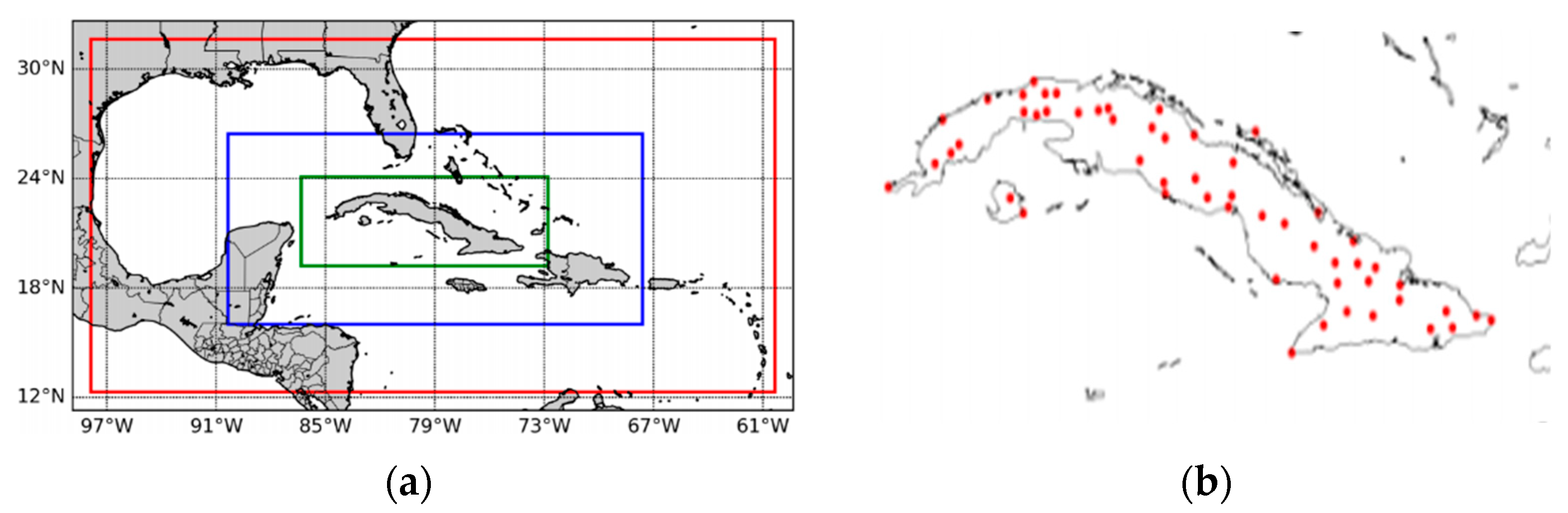
The physical configuration and the simulation domains of SisPI are shown in Table 1 and Figure 1a, respectively [1,2]. The evaluation is carried out for the domain with the highest resolution, that is, 3 km. This system generates four daily forecasts initialized at 0000, 0600, 1200, and 1800 UTC, taking the Global Forecast System (GFS) as initial data. In this study, the verification is conducted for the four initialization.

Table 1. Physical configuration of the WRF used in SisPI.

Parameters	Settings
Spatial resolution	Three nested domains of 27, 9, and 3 km of resolution
Nx	145, 162, 469
Ny	82, 130, 184
Nz	28, 28, 28
Domain center	21.8 N, 79.74 W
Time step	150s
Microphysics	WSM5,WSM5, double moment Morrison
Cumulus	Grell-Freitas, Grell-Freitas, not activated
PBL	Mellor-Yamada-Janjic, Mellor-Yamada-Janjic, Mellor-Yamada-Janjic

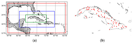
Figure 1. (a) Simulation domains for SisPI. The red square represents the simulation domain with 27 km of resolution, the blue square corresponds with 9 km resolution and the green one represents the domain with 3 km. (b) Meteorological surface stations used in the verification process.

Figure 1b shows the location of the 67 surface weather stations that were included in this study. The period to be evaluated was the year 2019.

For the verification were computed: the Mean Absolute Error (mae), the Mean Square Error (mse), the Mean Relative Error (mre), the Standard Deviation (std), Pearson’s Correlation Coefficient ($p_{corr}$), and the Adjustment Coefficient (ai); applying the cell-point verification approach [4]. All these metrics are computed for the temperature (t2), pressure (p), wind speed (v), relative humidity (hr), and precipitation (pr).

3. Results Discussion

The results obtained are presented below. Although the evaluation was developed for relative humidity, precipitation, wind, temperature, and pressure; the results obtained for the last two are not shown in this document. Furthermore, the bias and ai index graphics are not shown. The analysis focuses on the ability of the SisPI to represent the diurnal cycle. For this reason, throughout the document the results are shown in Local Hour.

3.1. Analysis for Relative Humidity

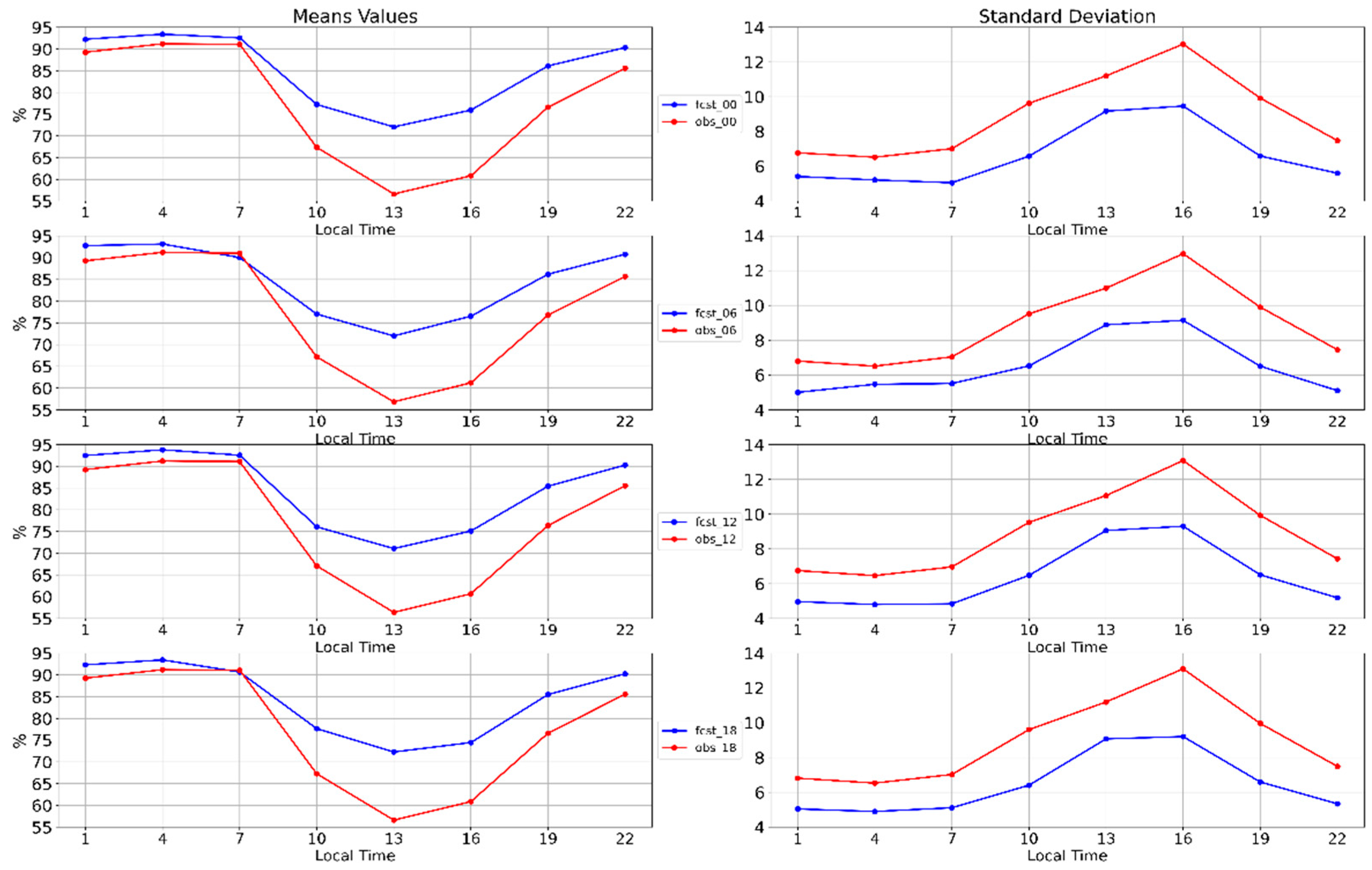
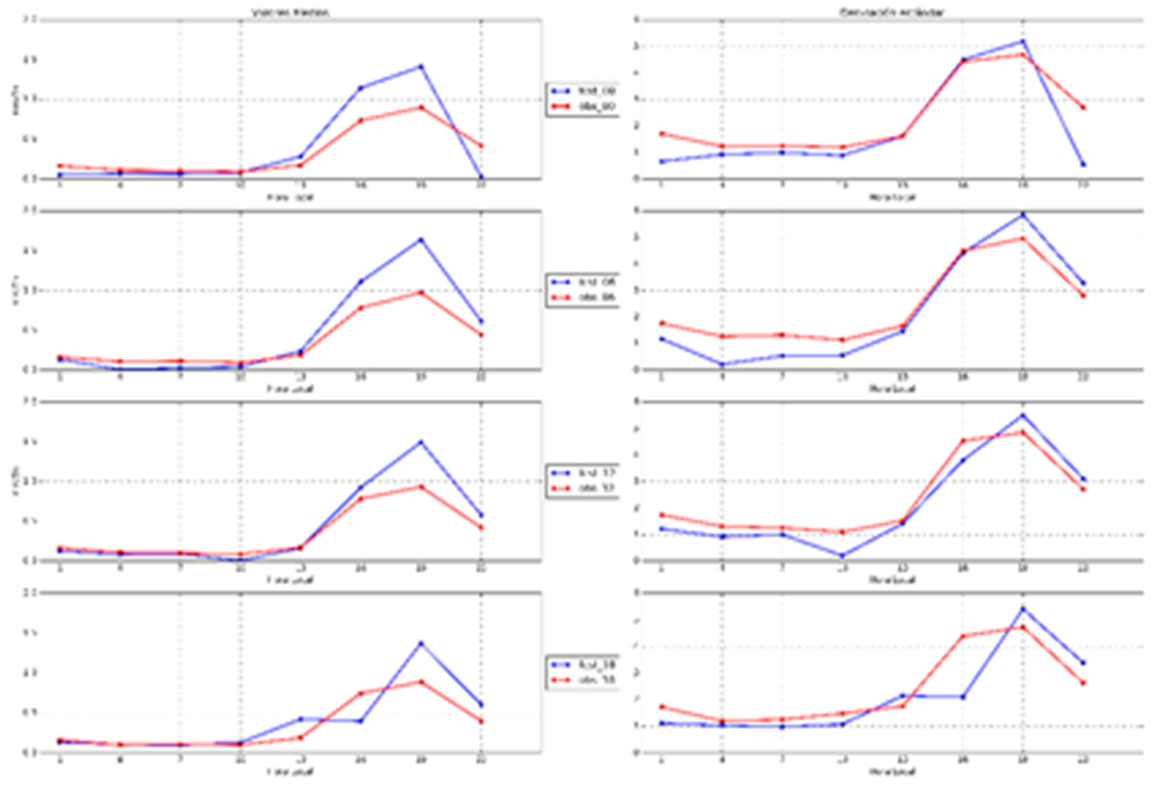
Figure 2 shows the mean values of the data and the standard deviations for relative humidity for 0000, 0600, 1200, and 1800 UTC.

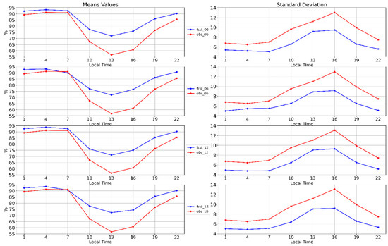
Figure 2. Average hourly values and standard deviation for relative humidity in %. The blue line is the forecast while the red line corresponds to the observations. From top to bottom, the panels present the results for the 0000, 0600, 1200, and 1800 UTC, respectively.

For the four initializations, it is observed that the lowest humidity is recorded during the daytime, reaching the minimum value at 1:00 p.m. (local time). An overestimation is observed by the model, showing the greatest differences between 10:00 and 16:00.

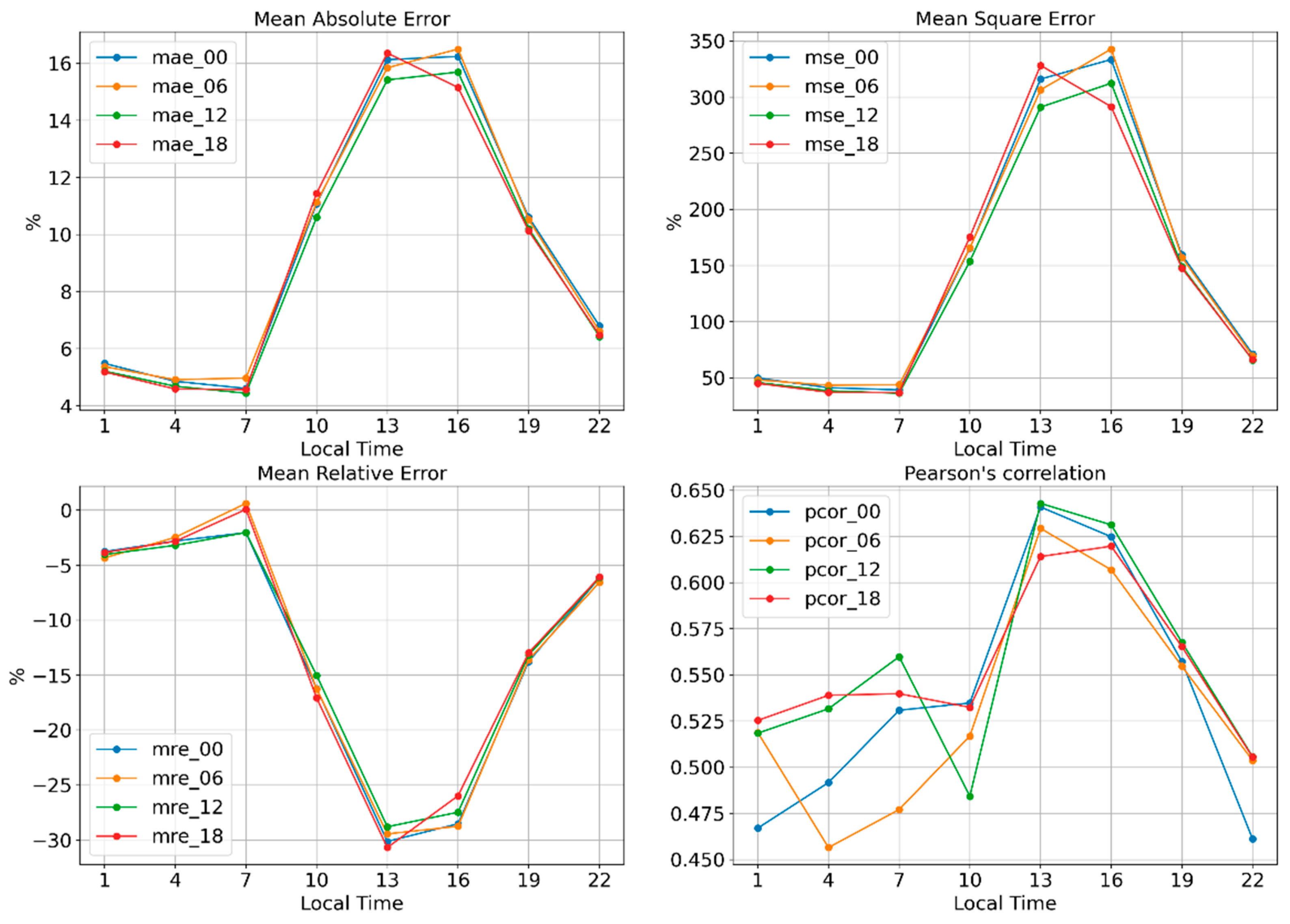
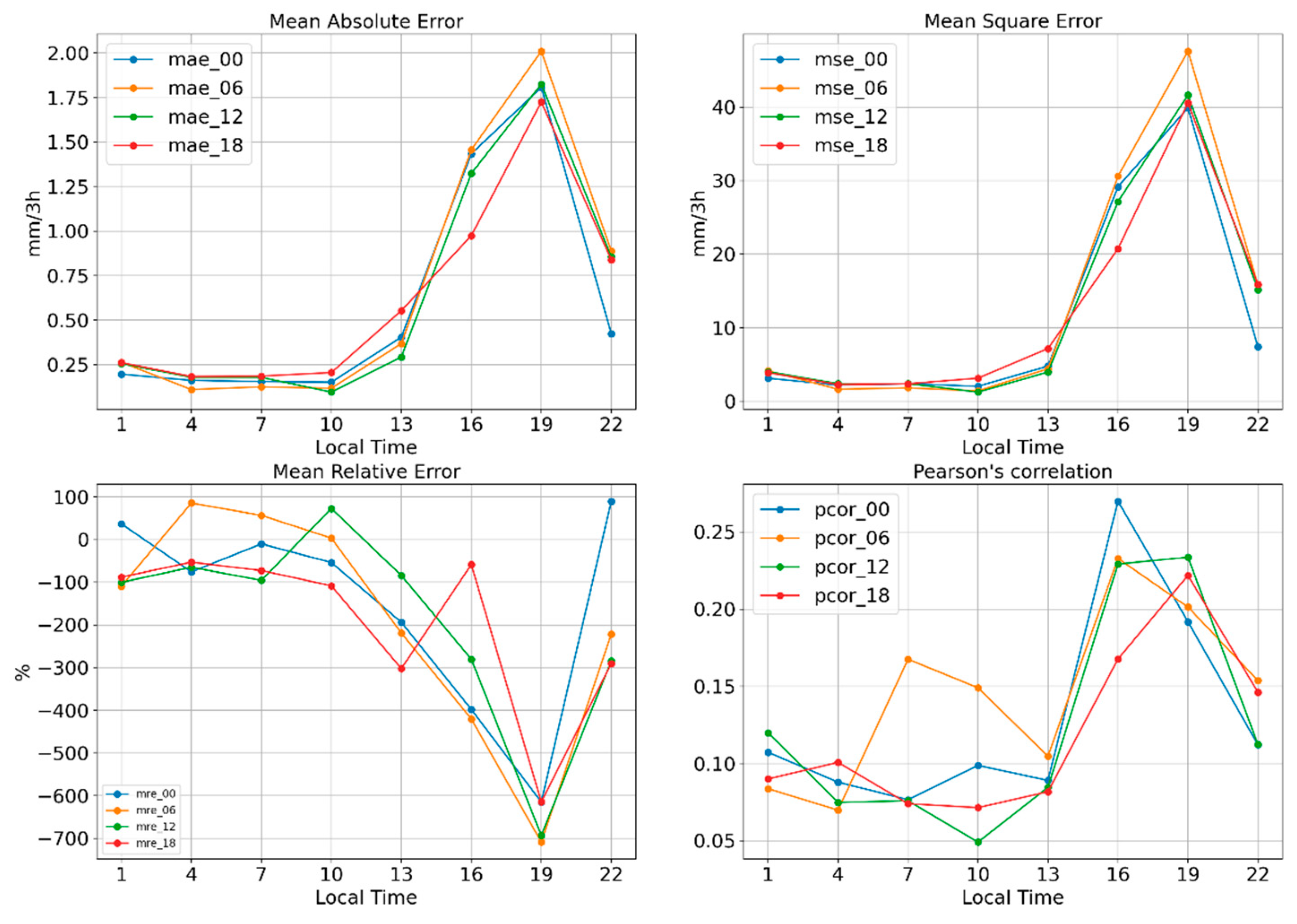
Figure 3 shows the mae, mse, mre, and Pearson’s correlation for relative humidity. It can be seen that the error metrics show similar behavior for all initialization. For each of them, the greatest errors are reached during the daytime (between 10:00 and 19:00) in which the relative humidity values are lower. Regarding the correlation, from 10:00, an increase in this value is observed, reaching a maximum at 13:00, which is between 0.60 and 0.65, and then begins to decrease until it reaches a minimum at 22:00. The diurnal cycle is well represented by SisPI despite the fact that the configuration used trends to overestimate the values of hr. On the other hand, there is not a marked difference between the SisPI’s runs with each initialization time, the run initialized at 1200 UTC slightly presents the better performance.

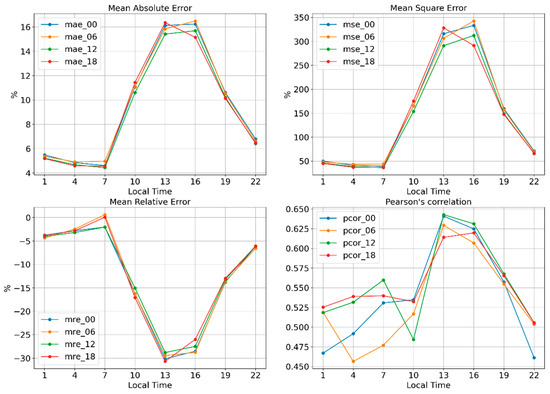
Figure 3. Error metrics(mae, mse, mre and $p_{corr}$) for hr.

3.2. Analysis for Precipitation

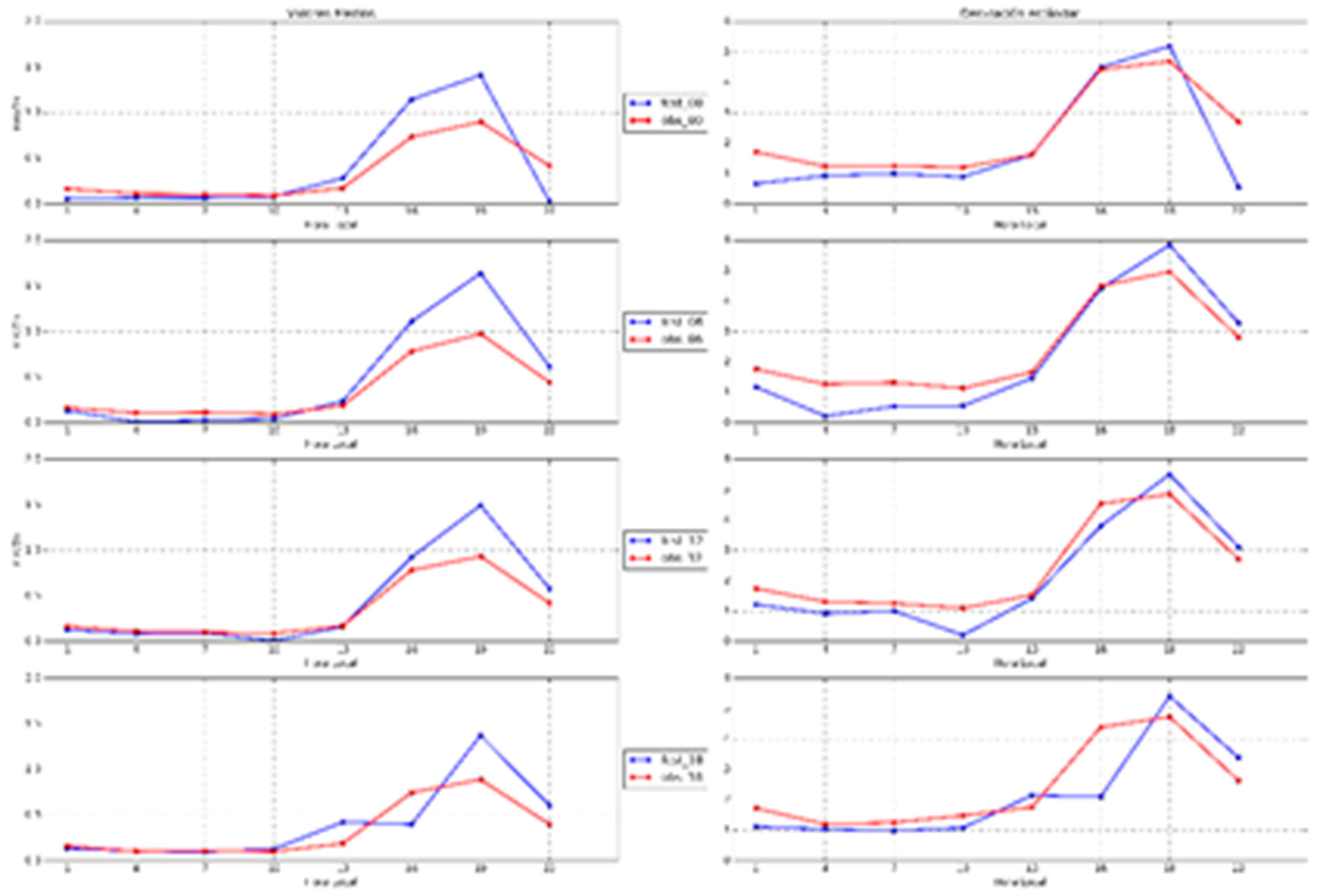
Figure 4 shows the mean values of the data and the std for precipitation in each forecast period. The forecast made by all initialization again overestimates the observed values, with the greatest difference in the afternoon (from 13:00 to 19:00), due to the fact that during this period the probability of rain increases because the daytime warming. In general, all the cases reflects the behavior of the rain in accordance with the observed behavior. In the graph it is observed that when the observations register an increase in the accumulated; the model does too. It can be seen that the deviation of the observed and predicted data is similar in all the forecast periods. Notice that the SisPI’s runs initialized at 1800 UTC presents the worst skill between 13:00 and 16:00. The latter is due to the spin up of the model.

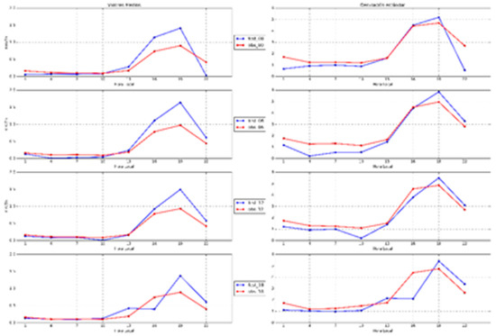
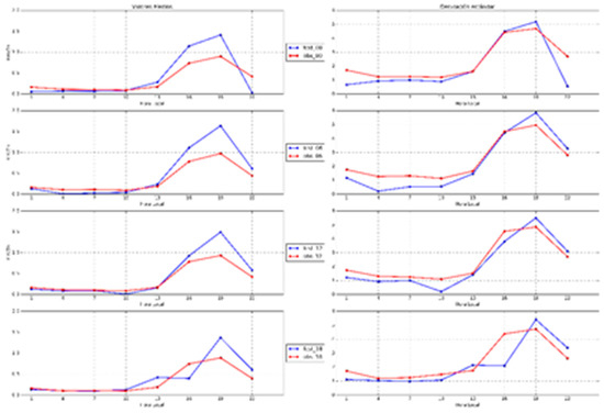
Figure 4. Average hourly values and standard deviation for precipitation in mm/3 h. The blue line is the forecast while the red line corresponds to the observations. From top to bottom the panels presents the results for the 0000, 0600, 1200, and 1800 UTC, respectively.

For pr, the biggest errors (Figure 5) occur in the afternoon. Negative mre values show that the model overestimates the precipitation values. Regarding the correlation $p_{corr}$, the values oscillate between 0.05 and 0.30, evidencing the poor ability of the model to represent the real amount of precipitation. The forecasts initialized at 0000 and 1200 UTC slightly exhibit the lowest error values.

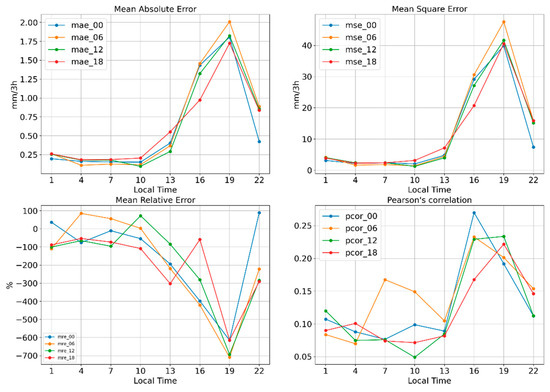
Figure 5. Error metrics (mae, mse, mre and $p_{corr}$) for pr.

3.3. Analysis for Wind Speed

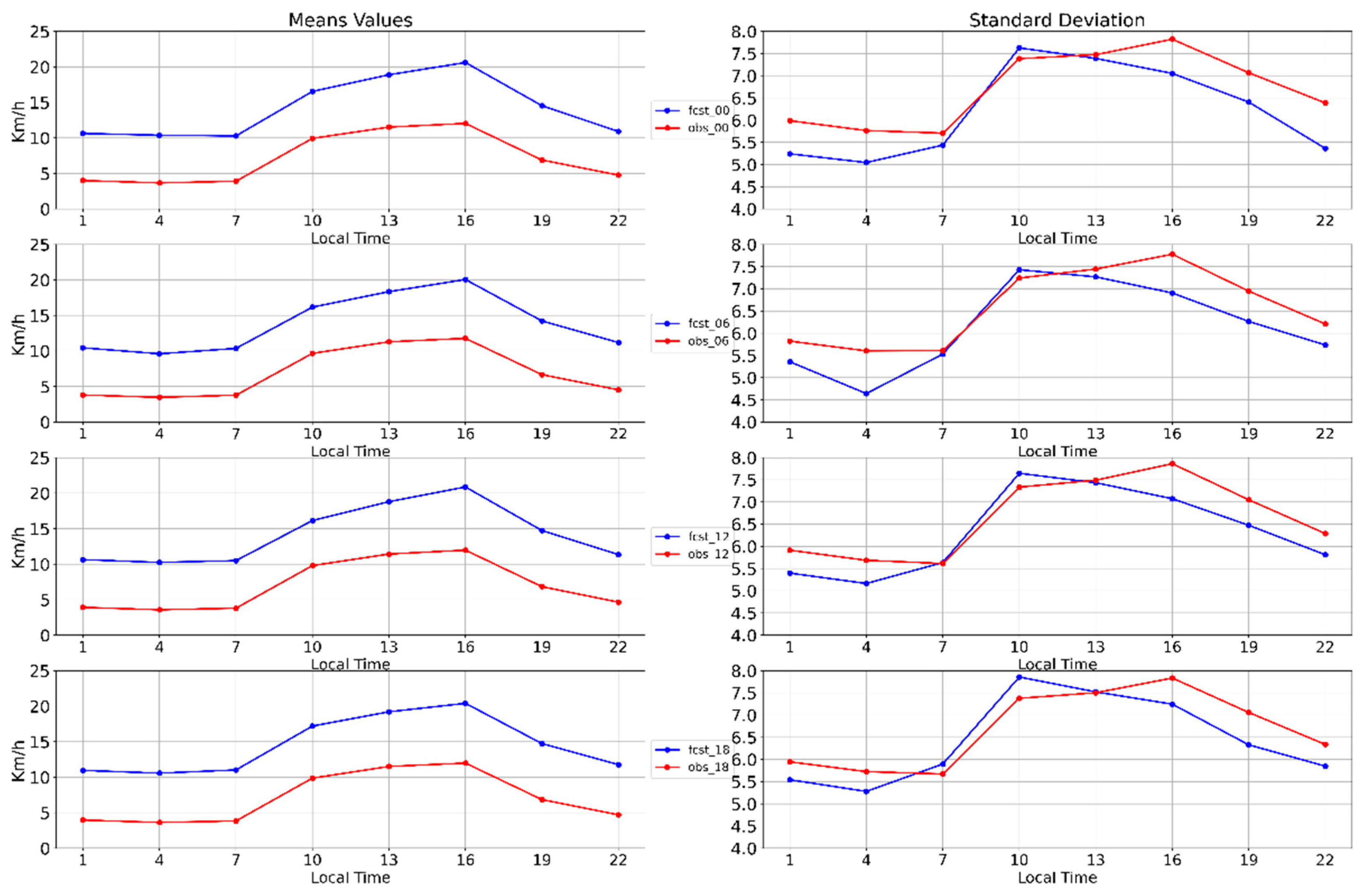
The verification results for wind speed are showed in Figure 6 and Figure 7. It can be observed that, in general, for all initialization, the standard deviation of the observed values is greater than the std of the predicted values. In each of the runs, it is observed that the highest values of wind speed are recorded in the daytime, reaching the maximum value at 16:00. An overestimation is observed by the model, showing the greatest differences between 10:00 and 16:00. The wind speed diurnal cycle is very well represented by SisPI.

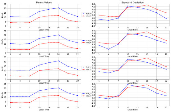
Figure 6. Average hourly values and standard deviation for wind speed in km/h. The blue line is the forecast while the red line corresponds to the observations. From top to bottom the panels presents the results for the 0000, 0600, 1200, and 1800 UTC, respectively.

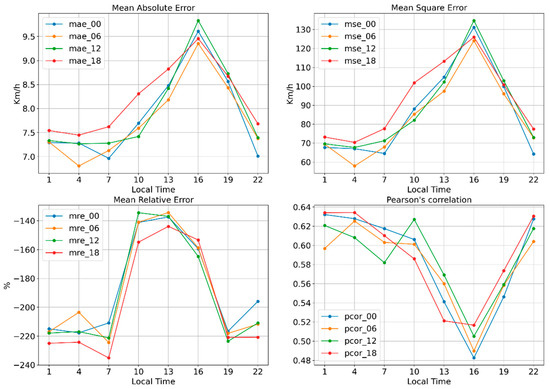
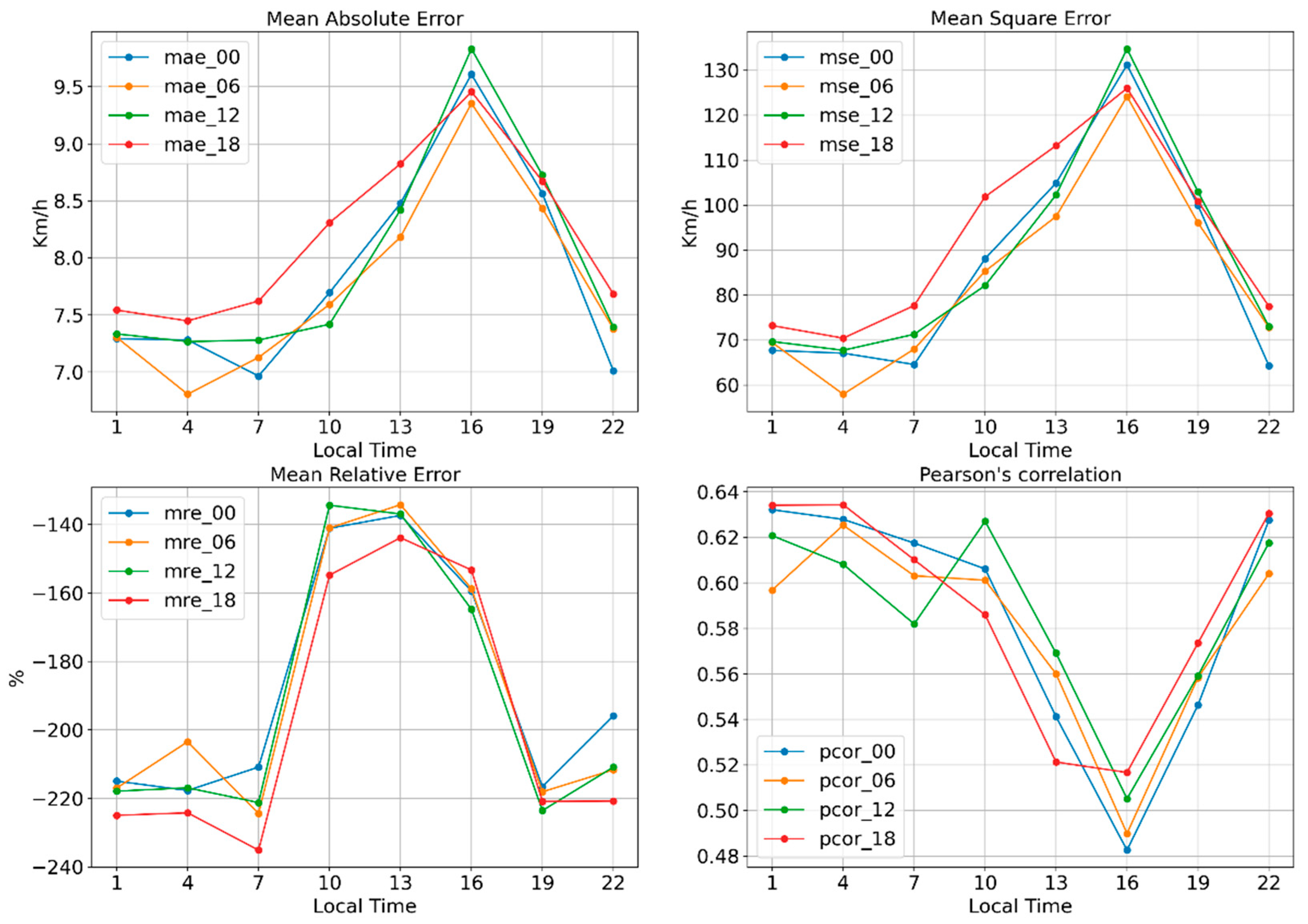
Figure 7. Error metrics (mae, mse, mre, and $p_{corr}$) for v.

In the Figure 7, it is observed that both the mean absolute error and the mean square error have a similar behavior. For both cases, the greatest errors are obtained in the afternoon, with a maximum at 16:00. The negative values of relative error show an overestimation by the model, obtaining the largest errors between 10:00 and 16:00, while the correlation reaches values that oscillate between 0.48 and 0.64, showing the minimum at 16:00 in all initialization.

4. Conclusions

• In this research, the proposed objectives are fulfilled, achieving a characterization of the forecast of the atmospheric variables at the surface level from the evaluation of the outputs of SisPI for all the stations of the country during 2019.
• The SisPI tool shows a good skill to forecast the diurnal cycle of the variables studied.
  • In relation to hr, the SisPI overestimates the values, having the greatest errors in the daytime;
  • For pr, the model presents the poorest skill highlighting the difficulty in forecasting the amount of precipitation;
  • In the case of v, also an overestimation by the SisPI is observed.
• In general, the SisPI’s run initialized at 1200 UTC yields the best results in terms of forecast accuracy.

References

- Sierra-Lorenzo, M.; Ferrer-Hernández, A.L.; Hernández-Valdés, R.; González-Mayor, Y.; Cruz-Rodríguez, R.C.; Borrajero-Montejo, I.; Rodríguez-Genó, C.F. Sistema automático de predicción a mesoescala de cuatro ciclos diarios. In Technical Report; Instituto de Meteorología de Cuba: Havana, Cuba, 2014. [Google Scholar]
- Sierra-Lorenzo, M.; Borrajero-Montejo, I.; Ferrer-Hernández, A.L.; Hernández-Valdés Morfa-Ávalos, Y.; Morejón-Loyola, Y.; Hinojosa-Fernández, M. Estudios de sensibilidad del sispi a cambios de la pbl, la cantidad de niveles verticales y, las parametrizaciones de microfısica y cúmulos, a muy alta resolución. In Technical Report; Instituto de Meteorología de Cuba: Havana, Cuba, 2017. [Google Scholar]
- Mesoescale & Microescale Meteorology Division. ARW Version 3 Modeling System User’s Guide. Complementary to the ARW Tech Note; NCAR: Boulder, CO, USA, 2014; p. 141. Available online: http://www2.mmm.ucar.edu/wrf/users/docs/userguideV3/ARWUsersGuideV3.pdf (accessed on 12 April 2020).
- WWRP/WGNE Joint Working Group on Verification. Forecast Verificacion-Issues, Methods and FAQ (pdf version). 2008. Available online: http://www.cawcr.gov.au/staff/eee/verif/verif_web_page.html (accessed on 15 May 2020).
Publisher’s Note: MDPI stays neutral with regard to jurisdictional claims in published maps and institutional affiliations. |
© 2021 by the authors. Licensee MDPI, Basel, Switzerland. This article is an open access article distributed under the terms and conditions of the Creative Commons Attribution (CC BY) license (https://creativecommons.org/licenses/by/4.0/).