
A Regression Line for a Laser Doppler Anemometer †


Abstract
:1. Introduction
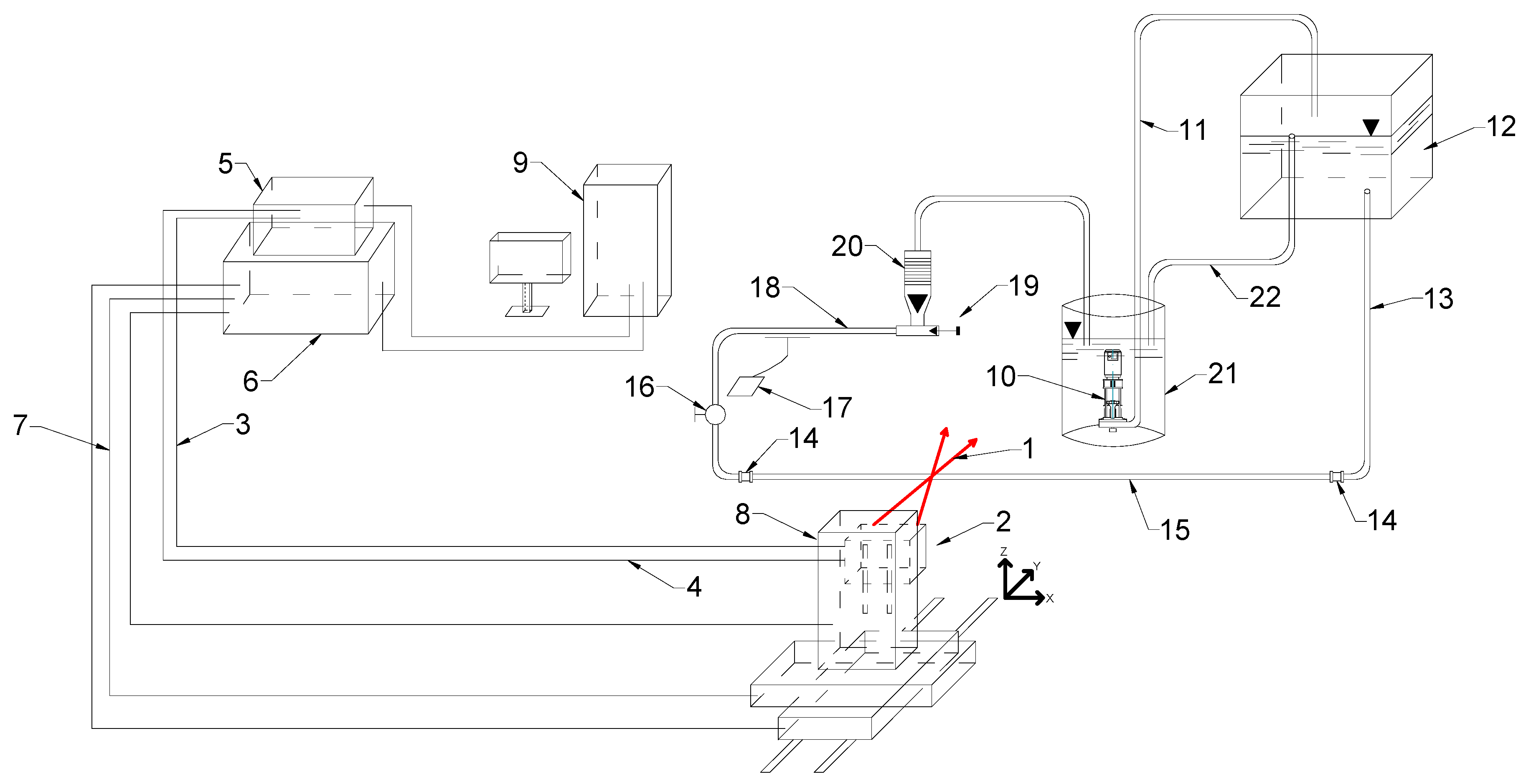
2. Methodology
3. Results and Discussion
Author Contributions
Funding
Conflicts of Interest
References
- Choudhury, B.; Chatterjee, P.K.; Sarkar, J.P. Review paper on solar-powered air-conditioning through adsorption route. Renew. Sustain. Energy Rev. 2010, 14, 2189–2195. [Google Scholar] [CrossRef]
- Abed, A.M.; Alghoul, M.A.; Sopian, K.; Majdi, H.S.; Al-Shamani, A.N.; Muftah, A.F. Enhancement aspects of single stage absorption cooling cycle: A detailed review. Renew. Sustain. Energy Rev. 2017, 77, 1010–1045. [Google Scholar] [CrossRef]
- Asfand, F.; Bourouis, M. A review of membrane contactors applied in absorption refrigeration systems. Renew. Sustain. Energy Rev. 2015, 45, 173–191. [Google Scholar] [CrossRef]
- Sehgal, S.; Alvarado, J.L.; Hassan, I.G.; Kadam, S.T. A comprehensive review of recent developments in falling-film, spray, bubble and microchannel absorbers for absorption systems. Renew. Sustain. Energy Rev. 2021, 142, 110807. [Google Scholar] [CrossRef]
- Madejski, J. (Ed.) Theory of Heat Transfer; Technical University of Szczecin Press: Szczecin, Poland, 1998. (In Polish) [Google Scholar]
- Hartley, D.E.; Murgatroyd, W. Criteria for the break-up of thin liquid layers flowing isothermally over solid surfaces. Int. J. Heat Mass Transf. 1964, 7, 1003–1015. [Google Scholar] [CrossRef]
- Bankoff, S.G. Minimum thickness of a draining liquid film. Int. J. Heat Mass Transf. 1971, 14, 2143–2146. [Google Scholar] [CrossRef]
- Mikielewicz, J.; Moszynski, J.R. Minimum thickness of a liquid film flowing vertically down a solid surface. Int. J. Heat Mass Transf. 1976, 19, 771–776. [Google Scholar] [CrossRef]
- Mikielewicz, J.; Moszynskl, J.R. An improved analysis of breakdown of thin liquid filmse. Arch. Mech. 1978, 30, 489–500. [Google Scholar]
- El-Genk, M.S.; Saber, H.H. Minimum thickness of a flowing down liquid film on a vertical surface. Int. J. Heat Mass Transf. 2001, 44, 2809–2825. [Google Scholar] [CrossRef]
- Perazzo, C.A.; Gratton, J. NavierStokes solutions for parallel flow in rivulets on an inclined plane. J. Fluid Mech. 2004, 507, 367–379. [Google Scholar] [CrossRef]
- Tanasijczuk, A.J.; Perazzo, C.A.; Gratton, J. Navier–Stokes solutions for steady parallel-sided pendent rivulets. Eur. J. Mech. B/Fluids 2010, 29, 465–471. [Google Scholar] [CrossRef]
- Ataki, A.; Bart, H.-J. Experimental Study of Rivulet Liquid Flow on an Inclined Plate. In Proceedings of the International Conference on Distilation & Absorpiton, Baden-Baden, Germany, 30 September–2 October 2002; GVC-VDI-Society of Chemical and Process Engineering: Baden-Baden, Germany, 2002; pp. 1–13. [Google Scholar]
- Charogiannis, A.; An, J.S.; Markides, C.N. A simultaneous planar laser-induced fluorescence, particle image velocimetry and particle tracking velocimetry technique for the investigation of thin liquid-film flows. Exp. Therm. Fluid Sci. 2015, 68, 516–536. [Google Scholar] [CrossRef] [Green Version]
- Teleszewski, T.J. Experimental investigation of the kinetic energy correction factor in pipe flow. E3S Web Conf. 2018, 44, 177. [Google Scholar] [CrossRef] [Green Version]
- Moffat, R.J. Describing the uncertainties in experimental results. Exp. Therm. Fluid Sci. 1988, 1, 3–17. [Google Scholar] [CrossRef] [Green Version]
- Szydłowski, H. (Ed.) Regression. In Theory of the Measurements; Państwowe Wydawnictwo Naukowe: Warszawa, Poland, 1981; p. 267. ISBN 83-01-01843-7. (In Polish) [Google Scholar]

Publisher’s Note: MDPI stays neutral with regard to jurisdictional claims in published maps and institutional affiliations. |
© 2021 by the authors. Licensee MDPI, Basel, Switzerland. This article is an open access article distributed under the terms and conditions of the Creative Commons Attribution (CC BY) license (https://creativecommons.org/licenses/by/4.0/).
Share and Cite
Weremijewicz, K.; Gajewski, A. A Regression Line for a Laser Doppler Anemometer. Environ. Sci. Proc. 2021, 9, 12. https://doi.org/10.3390/environsciproc2021009012
Weremijewicz K, Gajewski A. A Regression Line for a Laser Doppler Anemometer. Environmental Sciences Proceedings. 2021; 9(1):12. https://doi.org/10.3390/environsciproc2021009012
Chicago/Turabian StyleWeremijewicz, Karolina, and Andrzej Gajewski. 2021. "A Regression Line for a Laser Doppler Anemometer" Environmental Sciences Proceedings 9, no. 1: 12. https://doi.org/10.3390/environsciproc2021009012
APA StyleWeremijewicz, K., & Gajewski, A. (2021). A Regression Line for a Laser Doppler Anemometer. Environmental Sciences Proceedings, 9(1), 12. https://doi.org/10.3390/environsciproc2021009012