Bioinformatic Analysis of Metabolomic Data: From Raw Spectra to Biological Insight

Abstract

Metabolites are at the end of the gene–transcript–protein–metabolism cascade. As such, metabolomics is the omics approach that offers the most direct correlation with phenotype. This allows, where genomics, transcriptomics and proteomics fail to explain a trait, metabolomics to possibly provide an answer. Complex phenotypes, which are determined by the influence of multiple small-effect alleles, are an example of these situations. Consequently, the interest in metabolomics has increased exponentially in recent years. As a newer discipline, metabolomic bioinformatic analysis pipelines are not as standardized as in the other omics approaches. In this review, we synthesized the different steps that need to be carried out to obtain biological insight from annotated metabolite abundance raw data. These steps were grouped into three different modules: preprocessing, statistical analysis, and metabolic pathway enrichment. We included within each one of them the different state-of-the-art procedures and tools that can be used depending on the characteristics of the study, providing details about each method’s characteristics and the issues the reader might encounter. Finally, we introduce genome-scale metabolic modeling as a tool for obtaining pseudo-metabolomic data in situations where their acquisition is difficult, enabling the analysis of the resulting data with the modules of the described workflow.

1. Introduction

Metabolism is the currency of the physiological processes of all living organisms. The biomass that forms all organisms is a product of metabolism, as well as the chemical reactions that ensure its energetic viability and maintenance. The metabolome comprises all the small chemical compounds (metabolites) that are present in a biological system at a given moment [1]. These small compounds include sugars, amino acids, nucleic acids, lipids, fatty acids, phenolic compounds, and alkaloids. Due to metabolism being at the end of the gene–transcript–protein–metabolism cascade, the metabolome is the omics dataset that is closer to the phenotypic state of the organism under investigation [2]. This straightforward correlation facilitates the study of metabolism to possibly provide explanations for the mechanisms driving phenotypes where genomic, transcriptomic, or proteomic approaches cannot. One example of this are complex phenotypes, where the observed features are a product of a high number of small-effect alleles, rather than a few strong-effect mutations, which makes it difficult to establish connections between, for example, genome and phenotype [3]. In the context of pathogenic microorganisms, the possibility of examining their physiological state in a particular moment can provide insight into their virulence mechanisms. Some pathogens rely on the production of secondary metabolites to display increased virulence. For example, Pseudomonas aeruginosa produces rhamnolipids to form biofilms and spread across surfaces, and the secretion of these compounds serves as a means for reducing oxidative stress [4,5,6,7]. Other pathogens rewire their metabolic network to adjust to the stresses imposed by the infected host, diverting fluxes toward metabolic products that help to evade the immune response, serve as reserve resources against starving and protect against the host’s attacks. An example of this is Mycobacterium tuberculosis infection, which is characterized by a switch from carbohydrate to lipid use as a carbon source, an altered composition of the cell wall and an abrupt decrease in the growth rate [8,9,10]. These facts have contributed to an exponential increase in the interest in the application of metabolomic techniques in microbiological studies [11].

Metabolomic data are most frequently acquired with gas chromatography–mass spectrometry (GC-MS), followed closely by liquid chromatography–mass spectrometry (LC-MS) and nuclear magnetic resonance (NMR) [11,12]. GC-MS offers the advantages of the equipment being cheaper, easier to operate and less prone to maintenance issues. Additionally, retention times between runs are highly reproducible, making automated compound identification easier. Consequently, it is the gold standard for profiling primary metabolism [13,14]. An important drawback is that the sample needs to be volatilized prior to entering the chromatographic column, and is necessary to derivatize non-volatile compounds, therefore enabling the possibilities of the degradation of compounds and the formation of new ones as products of the heat [15]. On the contrary, LC-MS has the advantage that allows for the detection of more compounds than GC-MS, being able to acquire tens of thousands of features in a single run. The lack of methods available to determine the metabolite identity of all detected ions is, however, a major limitation [11]. Other advantages are a high sensitivity and, as it does not need compound derivatization, sample preparation is easier, faster, and cheaper [16]. The main drawback is that the chromatographic column does not behave exactly the same in separate runs. This causes compound elution times to naturally drift between runs [17], implying extra steps for identifying the identities of the peaks. Among the advantages offered by NMR are that it is non-destructive, allowing in vivo measurements, can provide information about the interactions of metabolites with macromolecules, has an easier workflow for performing isotope tracing than LC-MS and GC-MS, and is more reproducible [18]. The main drawbacks are less sensitive measurements, making challenging the detection of low-concentration compounds, and the needs for more physical space for the equipment and more specialized operators [18,19].

The bioinformatic analysis of metabolomic data can be divided into four main modules. The first module involves converting the raw spectra into metabolite feature data [20,21]. Metabolite feature data are tables of peak areas, where each row represents an analyzed sample, and each column, a metabolite. These peak areas are proportional to the relative abundance of the metabolite within the sample. To gain biological insight from the raw peak areas, several steps must be carried out, which can be grouped into the other three modules: peak area preprocessing, statistical analysis, and pathway enrichment. In the preprocessing module, missing values need to be imputed, and the unwanted experimental variability, removed. The statistical analysis module aims to identify associations between the biological factor of interest and the metabolite abundances. The final module, pathway enrichment, involves determining the metabolic pathways that appear to be perturbed across the biological factors of interest.

Although several approaches in the outlined workflow are specific for metabolomics, most of them have been adapted from the analytical routines used in quantitative disciplines that deal with high-dimensional data, such as transcriptomics and proteomics. This is especially relevant in the statistical analysis module, where all the discussed methods are either classic univariate methods, used to test hypotheses in a wide range of fields, or machine learning techniques, which have been applied to many different types of high-dimensional data. In the peak area preprocessing and metabolic enrichment modules, some of the discussed methods are specific to metabolomics, while others are shared with other omics approaches.

While there is considerable overlap, the particularities of each study lead to a lack of uniformity in metabolomic workflows, unlike in other omics disciplines. This is despite considerable efforts made to establish standardized practices [22]. Still, the modules that we outlined are common across most of metabolomic analyses. In this review, we discuss the different state-of-the-art approaches that fall within each one of them, detailing the particularities of each method, the situations where they can be used, the challenges that might appear and the issues that need to be considered. In the final section, we explore alternative approaches for cases where the access to metabolomic data is difficult, using genome-scale metabolic modeling to infer the metabolic state of organisms in particular situations.

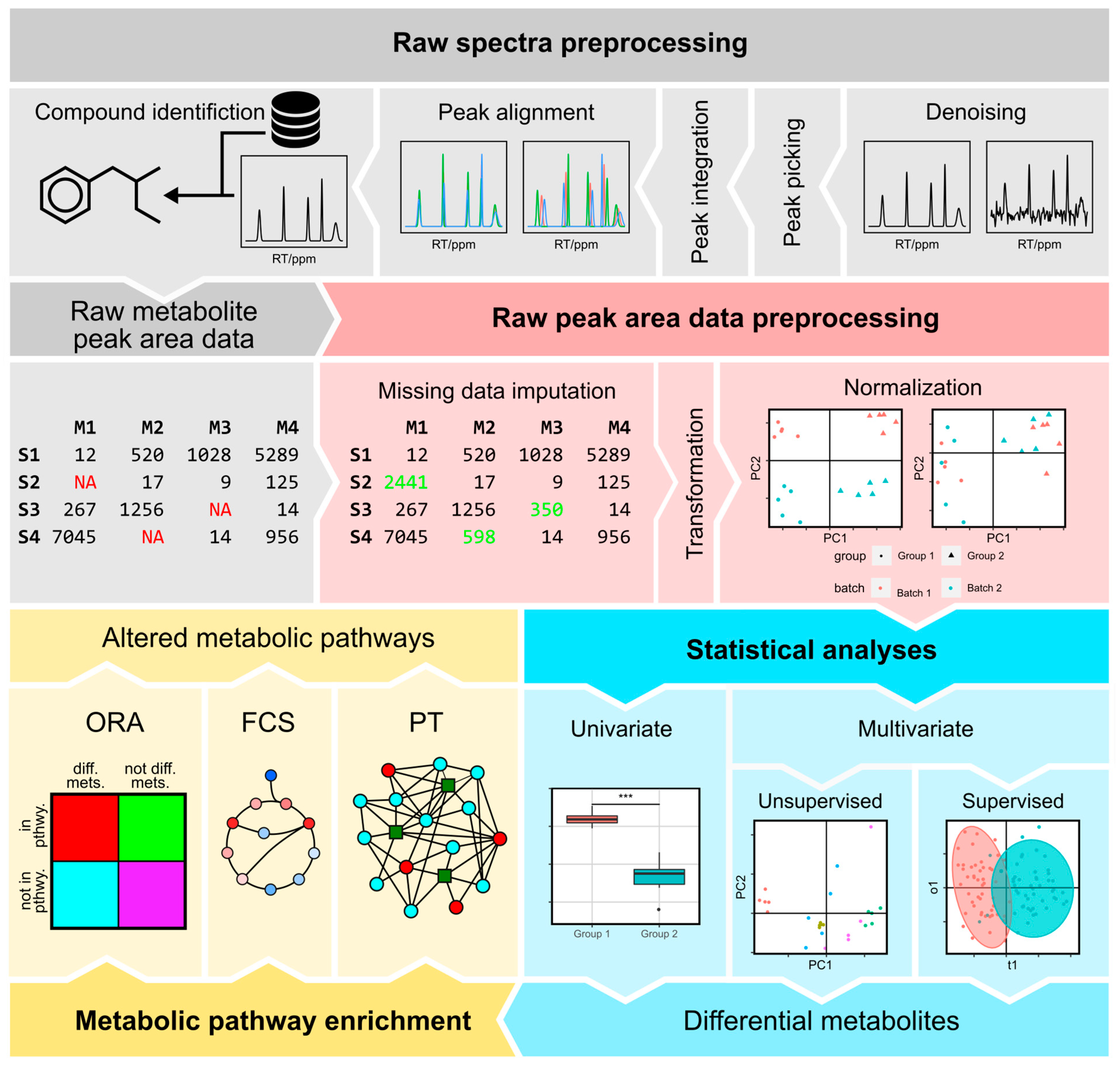
2. Raw Spectra Preprocessing

NMR and MS spectrum acquisition processes differ considerably. In NMR, data are registered by the equipment as decaying oscillations over time, called free induction decay (FID). FIDs are converted to the frequency domain through a fast Fourier transform, obtaining the NMR spectra. NMR spectra consist of frequency shifts relative to a reference compound, expressed in parts per million (ppm) and signal intensities [20]. In MS, the spectra dimensions are m/z ratio, intensity and retention time. These differences imply that the preprocessing necessary to go from the spectra to a metabolite abundance table will have some variations and will require specific software. Frequently, these packages are developed by the manufacturer of the experimental equipment, though there are open-source options available. In NMR, some commercial software used to perform spectra preprocessing are TopSpin (Brucker, Billerica, MA, USA), Mnova (Mestrelab, A Coruña, Spain) and Chenomx NMR Suite (Chenomx, Edmonton, AB, Canada), while popular open-source alternatives include nmrPipe and matNMR [23,24]. In MS, MassHunter (Agilent, Santa Clara, CA, USA) and Xcalibur (Thermo Scientific, Waltham, MA, USA) are two popular commercial packages. Among open-source options, MetaboAnalyst/MetaboAnalystR and XCMS are the most widely adopted ones [25,26].

The raw spectrum preprocessing steps typically include denoising, peak picking, peak alignment and compound identification. Differences in platforms also influence the level of automation. In GC-MS and NMR, due to the high reproducibility, these steps are highly automated, while in LC-MS some of them are more laborious and need more human intervention, especially compound identification.

2.1. Denoising

Data acquisition through NMR and MS introduces noise. Because of this, preprocessing workflows usually include a denoising step. In NMR, FIDs are commonly denoised using dimensionality reduction techniques such as single-value decomposition and principal component analysis (SVD and PCA, respectively) [27,28].

In MS, high-frequency noise is typically removed through smoothing, with common options being Savitzky-Golay, Gaussian or mean/median filters, as well as wavelet denoising [29,30]. For removing low-frequency baseline noise, common approaches include the use of linear, LOESS and LOWESS filters [29,31,32]. These approaches are also frequently used in the frequency domain in NMR to further improve the signal-to-noise ratio [20,27,30,32].

2.2. Peak Picking

After denoising, the next step is the extraction of the metabolomic features, a process known as peak picking. Peak picking consists of identifying and extracting the peaks that correspond to true single compounds among the whole spectra and determining the area under the peak, which is proportional to metabolite abundance. This latter step is known as peak integration. Peak picking is challenging, especially in NMR, due to the lower signal-to-noise ratio compared to MS and to the overlap of the peaks due to the lack of a chromatographic separation step [18]. There is a wide range of peak picking algorithms, ranging from the simplest ones, based on a search for local maxima, to the most sophisticated methods based on machine/deep learning [29,30,33,34].

2.3. Peak Alignment

During the acquisition of metabolomic data, non-linear shifts in spectra can occur due to physicochemical changes in the equipment across runs. In MS spectra, these shifts are mainly observed in the retention time, which is known as column drift. In NMR, shifts are observed in the ppm axis. As previously discussed, column drift is especially notable in LC-MS. Therefore, to integrate the detected metabolic features across different samples, it is necessary to perform a peak alignment step. Time warping and segmenting algorithms are frequently used for this purpose, both in MS and NMR [35,36]. Binning is also used in NMR for this purpose. Here, the spectra were divided in small buckets, which, ideally, contained single peaks, while allocating the ppm drift across samples [37].

2.4. Compound Identification

Compound identification is performed by mapping the spectra to libraries such as NIST, HMDB and METLIN [38,39]. In GC-MS, this step is highly automated, given the reproducibility of retention times, which allows the mapping of spectra to the libraries with high accuracy. In LC-MS and NMR, the variations in retention times and ppm contribute to a less straightforward identification, often requiring the manual annotation of some peaks [40]. It is common that the metabolite identification step is not restricted to raw spectrum preprocessing: differential analyses can be performed using metabolic features with both known and unknown identities, for later revisiting the compound identification, focusing on the unknown peaks significantly associated with the phenotype.

3. Peak Area Preprocessing

After raw spectrum preprocessing, a metabolite table of peak areas will be generated, where rows and columns correspond to samples and metabolites, respectively. These peak areas are proportional to relative metabolite abundance. This table will present two issues: some metabolites will have missing values in some samples, and there will be variability due to technical errors. Regarding the missing values, it needs to be determined if these metabolites are truly absent in the sample or below the limit of detection, or there was some error in the metabolite detection or in the determination of the peak, and their abundances need to be inferred. This process is known as missing value imputation. The handling of the technical variation introduced during sampling preparation and data acquisition is accomplished in the normalization step.

3.1. Missing Value Imputation

Metabolomic data acquired with mass spectrometry (MS) present missing values at a proportion that can be as high as 20% and affect 80% of the detected metabolites [41]. These missing values can interfere in the statistical analyses performed downstream, making it important to address them during preprocessing [42]. The strategies for handling missing values in metabolomics are borrowed from other omics disciplines, particularly transcriptomics. Prior to imputation, variables with a high proportion of missing values are typically removed from the dataset. An example of this approach is the “80% rule”, where metabolites with more than the 20% of missing values are removed from the dataset [43]. Samples with more than 80% of the variables missing are also filtered out.

For after the prefiltering, there are various approaches for dealing with missing values, some more sophisticated than others. These can be broadly divided into three categories [44]. The simplest methods fall under single-value imputation, which includes the imputation using (1) the mean, (2) the median, (3) the minimum, (4) the minimum/2 or (5) zero. Imputation using the mean and the median of the non-missing values of a given variable assumes that the origin of the missing values is random, caused by errors during the sample preparation or detection. Conversely, imputation using the minimum, the minimum/2 and zero assume that the value is missing because it is below the limit of detection. As a result, these methods do not determine the cause of each missing value observation. Moving to more complex approaches, we find imputation methods based on local structures. Some examples are random forest and k-nearest neighbor imputation methods [45,46,47]. These methods infer the imputed value based on the values of the same variable in other samples that are similar according to the rest of the variables. Consequently, they can, to some extent, determine if a missing metabolite is below the limit of detection or was not detected due to some other issue. The third category includes methods based on global structures, which infer missing values based on the “shape” of the vector space determined using the metabolomic matrix. In these methods, the missing values are iteratively estimated until they converge. Options in this category include methods based on Single-Value Decomposition (SVD) [48], on Bayesian Principal Component Analysis (BPCA) [49] and on Probabilistic Principal Component Analysis (PPCA) [50].

3.2. Normalization

After missing value imputation, an important step is to normalize metabolomic data to remove the technical variation that might have been introduced during the experimental procedure. The sources of this variation are diverse, including human error, differences in temperature or atmospheric conditions, and variation within and between instruments, among many other sources. When samples are acquired in short intervals of time, the produced variation may or may not have a large impact. However, when measurements are performed in different batches separated in time these differences can become considerable. Samples that have been run in the same batch were subjected to the same conditions determined at the moment when the analysis was performed and, therefore, have common traits that are not related to the biological factors of interest. This is known as the batch effect [51]. In order to help distinguish batch effect from true biological variation, it is important to evenly split the samples belonging to the different biological groups across different batches during the design of the experiment in the data acquisition step.

Compared to transcriptomics or proteomics, where, commonly, all abundances are normalized to a single value (i.e., the total amount of transcripts or proteins in the sample, the mean, the median or a value obtained based on a set of housekeeping features) [52,53,54,55], there is no standard method for dealing with non-biological variability in metabolomics [56,57]. Furthermore, the outcome of the experiment can vary greatly depending on the chosen normalization method [58]. Consequently, a good practice is to test different methods and compare their performances [59].

3.2.1. Normalization Methods

Normalization methods can be classified as pre-acquisition, or preventive, and post-acquisition, or curative [60]. Pre-acquisition methods consist in diluting the samples to bring all of them to the same global concentration, prior to sample preparation and analysis. In the case of microbial metabolomics, the most common approach is taking all the samples to the same optical density (OD, absorbance at 600 nm) before metabolite extraction [61]. For other cases, some alternatives are normalizing to the total dry weight, to the number of cells or to the total DNA or protein quantity in the sample [56]. Post-acquisition methods are mathematical procedures that aim to remove the technical variation after the analytical process [56]. Differences in the performance between pre- and post-acquisition methods have been reported, with many post-acquisition methods failing to overcome non-linear variability [62]. However, even performing pre-acquisition normalization, differences in the analytic equipment conditions between runs can still produce variation during data acquisition, which still needs to be handled [63]. So, a combination of both approaches is advisable.

Before post-acquisition normalization, it is also advisable to transform the data, as metabolite abundances tend to have a right-skewed distribution [64]. Log transformation is the most used approach but may become problematic when dealing with small values, because as they approximate to zero, log transformation tends toward minus infinite. An alternative to overcome this problem is the power transformation, which consists of raising the values to the power of a rational number, commonly 1/2 [65]. Another solution that allows the use of log transformation consists of adding a small number c to all the values before transformation to avoid the occurrence of zeros.

Regarding post-acquisition methods, there are different alternatives. In this review, we will cover a selection of them. As with missing value imputation, there are some normalization methods that are more sophisticated than others. The less sophisticated ones are inherited from transcriptomics and proteomics. These are the scaling normalization methods, which consist in subtracting or dividing each metabolite abundance by a single value. Some options are the mean, median or sum of all the peak intensity values for the given sample [66]. When the number of differential compounds is low, these methods can be efficient solutions. But they present the problem that on many occasions, the increase in the abundance of a particular group of metabolites is not accompanied by a decrease in another group (self-averaging property does not occur). So, if there are many differential compounds, normalizing to a single value obtained from the total peak values can introduce differences in some metabolites that are not actually there [67].

With an increased level of sophistication, there are the normalization methods that rely on the spiking of one or several internal standards in the sample. Depending on whether it is desired to capture differences only in instrumental variation, or also in extraction efficiency, the internal standards can be added just before running the analytical step, or before the metabolite extraction, respectively. The compounds used in the latter case are referred to by some authors as surrogate standards. The compounds typically used as internal standards are isotopically labeled versions of known metabolites [68]. The simplest of the normalization methods within this family is based on a single standard and is simply referred to as the IS (internal standard) method [69]. Here, the peak intensity of each metabolite in each sample is normalized to the peak intensity of the internal standard, either by dividing each metabolite by this value or by subtracting it from each metabolite peak intensity [66,69]. The main drawback of this method is the assumption that all the metabolites are affected equally by the technical variation, which might not be always appropriate as variation can be influenced by their chemical properties. Therefore, the chemical properties of the standard might introduce variation due to matrix-specific effects [67]. A solution to these issues is to add more than one internal standard. The simplest approach using several internal standards is the retention index (RI) method. Here, standards with different retention times are added to the samples. Each analyte is then normalized to the quality control metabolite with the closest retention time [43]. However, technical variation might arise from sources other than retention time. Because of the few sources of variability that the scaling, IS and RI methods account for, they struggle to remove technical variation in complex experimental designs accounting for several batches.

Several normalization methods use statistical modeling to capture the different sources of technical variation, which allows them to deal with batch effects. NOMIS (Normalization using the Optimal selection of Multiple Internal Standards) aims to determine the covariance between the internal standards and the analytes through multiple linear regression, and then removes this covariance from the analytes [67]. This way, the standards of a larger covariance with each metabolite are given more weight in the normalization, effectively selecting the optimal standards for the normalization of the given analyte [67]. Despite this improvement, the internal standards could still be affected by cross-contribution, a phenomenon that is observed when different analytes that co-elute in the chromatographic column, producing interference in the measurement [70]. The Cross-contribution Compensating Multiple standard Normalization (CCMN) method overcomes this issue by performing the normalization in several steps [71]. First, the variation introduced by the experimental design that is cross-contributed through the analytes to the standards is removed via multiple linear regression (MLR). These cross-contribution-free standard values are then used to perform normalization [71]. Instead of using internal standards for normalization, another option is to use non-changing metabolites, which are present in the biological samples and, therefore, are exposed to technical variation but are uncorrelated to the biological factors of interest. RUV-2 (remove unwanted variation, 2-step) method uses this approach [63,72]. Here, the unwanted component factors are estimated through the single-value decomposition (SVD) of the non-changing metabolite matrix, to later fit a linear model to each metabolite using as explanatory variables both the factors of interest and the unwanted component factors [63,72]. These non-changing metabolites can be determined through statistical analysis or by determining which are the metabolites that correlate more with the standards (if included in the experiment) [63]. Non-changing metabolites have also been used with success with other normalization methods such as CCMN instead of internal standards [73]. Another category includes the methods based on quality control (QC) samples, which are analyzed before and after and scattered at regular intervals throughout each batch. These methods use the shifts between the measures of a QC sample to correct the values obtained from the test samples. A representative method of this class is quality control–based robust LOESS (locally estimated scatterplot smoothing) signal correction (QC-RLSC) [74]. These QC samples can be either pooled samples, obtained by combining small aliquots of all the samples in the study, or commercially available QC samples made of combinations of different biofluids [74,75,76,77]. Pooled QC samples offer the advantage that they contain the same metabolites that can be found in the individual samples, constituting the average of all the samples. The use of commercially available QC samples often implies metabolic information losses due to metabolites being detected in the test samples but not in the QCs. Consequently, these metabolites will not be considered in downstream analyses. However, in long studies where sample preparation and data acquisition start before the collection of all the samples, the use of commercially available QC samples might be necessary [74]. Finally, blank samples are another type of QC sample that, while not directly related to normalization, are important in the assessment of the reproducibility of the analyses. These samples consist of either only solvent or the matrix of the sample, with optional internal standards spiked. Furthermore, the use of these samples allows us to identify background compounds that should be excluded from downstream analyses [78]. The use of QC samples also serves for preparing the equipment for the analysis of the test samples, as the first few injections in a run tend to be poorly reproducible [74,79,80].

Table 1. Normalization method families and some examples.

Scaling Methods	Internal Standard/Nonchanging Metabolite-Based		QC Sample-Based
	Scaling	Statistical Modeling
mean median sum	IS RI	NOMIS CCMN RUV-2	QC-RLSC

summarizes the post-acquisition normalization methods discussed in this section. These normalization methods are included in the NormalizeMets and MetaboAnalystR R packages [66]. However, while these methods are representative of the different approaches used for dealing with technical variation, there are additional approaches beyond those covered here.

3.2.2. Assessment of Post-Acquisition Normalization Effectivity

Each one of the post-acquisition methods mentioned here solves an increasing number of issues that metabolomic data can present, and, consequently, there is an increment in complexity as well. Depending on the experimental implementation, the use of some methods might be more appropriate than others, as in some cases, using excessively complicated methods may be overkill. For example, in cases where the number of differential metabolites is small, such as in drug screening, scaling methods or the IS method might be enough [70]. But in comparisons involving multiple differential metabolites, an increasing level of complexity is probably needed. Thus, it is recommended to test the performances of different methods to assess which is the one that best suits the dataset. There are different approaches to determine this, all of them complementary.

One approach is to evaluate the tightness of the replicates. A way of assessing this is by comparing the average distance of each sample to its replicates and to the average distance of each sample to the samples that are not replicates. A good normalization method should minimize the distance between replicates while maximizing the distance between groups. So, a scatterplot showing the average within- and between-group distances in the x and y axes for each one of the tested normalization methods can easily show which of them is optimizing these distances (Figure 1A). The tightness of replicates can also be determined using silhouette statistic [81]. A silhouette can be computed for each one of the data points in each one of the datasets generated with the tested normalization methods, considering the cluster as the group of replicate samples (Figure 1B). The best-performing normalization method, in terms of tightness of replicates, will display a distribution of silhouettes with a lower standard deviation and higher median.

Another option is to use within and between relative log abundance (RLA) plots [63]. Within-group RLA plots are boxplots of groupwise standardized log metabolite abundances, obtained by subtracting the median of the log abundances of each metabolite in the replicated samples to each sample. Within-group RLA plots show the tightness of the replicates achieved using the normalization method: all the samples should have a median within-group relative abundance close to zero and low standard deviation. For obtaining across-group plots, the median log abundance of each metabolite across all the samples is subtracted from the log abundance of each metabolite in each one of the samples. The obtained boxplots show the variability between the groups of replicates; replicates should not vary a lot, but differences between groups of replicates should be observed. If within-group RLA plots show a big proportion of the samples with their medians being different from zero, it means that the normalization method is not removing the unwanted variation properly. If within-group RLA plots look as expected, but across-group RLA plots show no difference between groups, it is a sign that the normalization method is removing the technical variation and also an important part of the biological variation [59].

Multivariate non-supervised approaches such as principal component analysis (PCA) or hierarchical clustering analysis (HCA) can also be used to see if the samples aggregate according to their replicate structure, or if instead, they group by batch. The results obtained with the unnormalized dataset and each one of the normalization methods can be compared to determine which of the methods yields tighter replicates and better removes batch effects [71].

Another approach for assessing the adequacy of the normalization method is, if there are metabolites that are known beforehand to be differential between the levels of the biological factor of interest (positive control metabolites), to rank the statistically significative metabolites before and after normalization and see if they are among the top significatives after normalization, meaning that the biological variation has not been removed [82].

The normalization diagnostic procedures discussed in this section can be performed using R statistical software with its included plotting features, or alternatively, with the ggplot2 package. RLA plots can be obtained easily with the NormalizeMets R package [66]. In Python, the SciPy and Matplotlib libraries can be used for this same purpose [83,84].

4. Statistical Analysis of Metabolomic Data

Once the metabolomic data have been normalized with the best-performing method, different approaches can be used to determine which are the metabolites that are associated with the studied biological factors. Depending on the nature of these biological factors and the complexity of the relationship between them and the metabolic features, different approaches can be used.

4.1. Univariate Analyses

Univariate analyses are the simplest statistical methods for identifying metabolites associated with specific biological factors, such as phenotypes or experimental conditions. These tests involve evaluating the association between individual metabolites and factors of interest [85]. The choice of test depends on the nature of the studied biological factor—whether categorical or quantitative—and the distribution of the data (

Table 2. Univariate tests classified according to the type of biological factors they can deal with.

Quantitative Factors	Categorical Factors
	Parametric		Non-Parametric
	2 Classes	>2 Classes	2 Classes	>2 Classes
Simple linear regression	Student’s t test Logistic regression (Wald test)	ANOVA	Mann–Whitney U test	Kruskal–Wallis test

). For quantitative factors, simple regression is recommended, while for categorical factors, the Student’s t-test, logistic regression or the Mann–Whitney U test can be used for two categories, and ANOVA and Kruskal–Wallis tests for more than two categories [85]. In logistic regression, significance can be assessed with a Wald test [86]. The Student’s t-test, logistic regression and ANOVA assume a normal distribution of metabolite abundances (parametric), while the Mann–Whitney U and Kruskal–Wallis tests do not (non-parametric). Metabolite datasets typically contain from tens to hundreds of variables. Consequently, when conducting univariate analyses, p-value correction is necessary to mitigate the increased risk of false positives resulting from multiple tests [87].

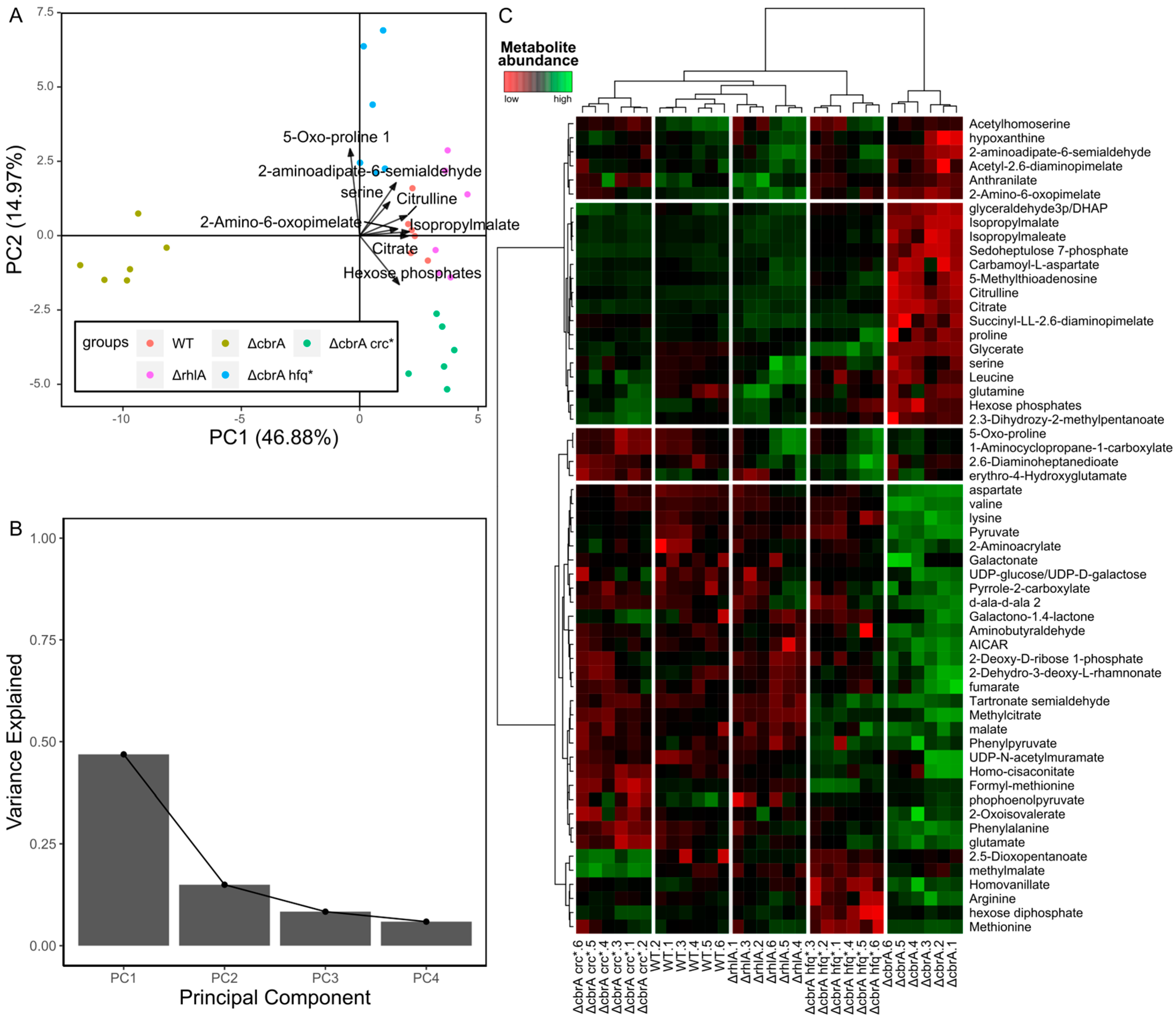
4.2. Multivariate Analyses

Multivariate analyses differ from univariate analyses in that they test the association of all independent variables to response variables simultaneously. In metabolomic experiments, metabolite abundances are measured outcomes and are not usually manipulated. Therefore, they have the role of dependent variables according to the experimental design (as is considered in univariate analysis). But metabolites are not independent entities because they are connected through the metabolic network. Consequently, we expect that the different phenotypes being compared or the adaptation to the experimental treatments may result from a coordinated change in multiple metabolites. In using metabolite abundances as independent variables in multivariate analyses, it is possible to assess the relationships between the different variables, providing insight into their interaction in relation to a particular biological factor [88]. Another advantage is that only one test is performed for all variables, avoiding the need for multiple hypothesis tests. Multivariate analysis methods can be broadly divided into supervised and unsupervised types, depending on whether information about the response biological variable is provided to the method.

4.2.1. Non-Supervised Multivariate Analyses

Non-supervised multivariate analyses are a good way of visualizing the structure of the dataset. In metabolomics, the most used method within this category is principal component analysis (PCA). PCA rotates the data in the multidimensional space determined by the variables, bringing the data to a new coordinate system where the variance is maximized across its axis (the principal components). The typical graphical representation of the PCA is a score plot, which is a scatterplot of the sample values for two principal components, usually the first and the second, as they contain most of the variance in the dataset. With this representation, it is possible to see the clustering of the samples according to their metabolite abundances. Ideally, this would correspond to the biological factors of interest, if variation between the samples sharing the same phenotype is small enough compared to the variation between samples belonging to different biological groups [89]. It is common to overlay the vectors of the loadings of the represented principal components of some or all the variables used in the PCA, as loadings reflect the contribution of each variable to the correspondent principal component. This combination is designated as a biplot (Figure 2A). Another common representation of PCAs is a multi-score plot, which arranges the score plots of a combination of a selected number of principal components. This helps to identify groupings that might not be visible in the first two components. Finally, Scree plots show the amount of variance included in the sorted principal components as a bar plot (Figure 2B).

Another commonly used non-supervised multivariate approach is hierarchical clustering analysis (HCA). In HCA, a determined distance metric, usually in Euclidean distance, is obtained between pairs of samples, and the samples are iteratively aggregated into clusters, according to a criterion determined using the linkage method. In metabolomics, HCA is usually graphically represented in heatmaps, where metabolites are clustered vertically, and samples, horizontally. This results in a row dendrogram and a column dendrogram, usually containing the metabolites and the samples, respectively, and a tile plot in between, where the colors reflect metabolite abundance (Figure 2C). With this visual representation, it is possible to easily visualize groups of samples that have similar metabolic profiles, and groups of metabolites that have similar abundance patterns across groups of samples. This can reveal alterations in metabolic pathways correlated with sample grouping.

PCA score plots have the advantage that, as principal components are sorted according to how much variance they contain, low-correlated information is filtered out. Therefore, PCA plots usually present a cleaner representation of the groups. However, this can be a disadvantage when there is biologically relevant information included in the principal components other than those represented in the score plots. In an HCA heatmap, on the other hand, all the information of the dataset is included, which makes it easier to visualize the influence of the variables over the sample aggregation but causes the grouping to be noisier. Another disadvantage of HCA is that it will always output some grouping, despite the existence (or not) of any pattern. PCA score plots, on the contrary, would display, in this situation, a sparse cloud pattern, where all the samples appear distributed without any structure in the bidimensional space.

An approach used to assess the stability of the observed grouping using HCA is consensus clustering, where several iterations of the clustering algorithm are performed, excluding a random number of samples each round. This method requires a prior indication of the number of groups (k) that the samples are being clustered into. In order to determine the number of significant groups, different ks are tested and, for each k, a consensus matrix is obtained. This consensus matrix indicates how many times each pair of samples was clustered together, divided by how many times they were selected together in all iterations. Ideally, this matrix would be composed of zeros and ones. In determining how far the obtained consensus matrix is from the ideal one, the optimal number of clusters can be obtained. This can be accomplished by comparing the CDF (Cumulative Distribution Function) curves of each k. The original metric used for this comparison is delta K, which is the relative change in the area under the curve. However, the proportion of ambiguous clustering (PAC) has been shown to outperform delta K [90]. The PAC quantifies the proportion of pairs of samples that fall in the middle segment of each CDF curve, which indicates that they cluster ambiguously. The PAC is computed by subtracting CDF_k(u₁) from CDF_k(u₂), and the u₁ and u₂ commonly used are 0.1 and 0.9, respectively. With both metrics, the ‘elbow’ method is the most commonly used to select the best k. This approach is, however, rather subjective, so different alternatives have been proposed in order to determine the number of significant clusters more objectively. An example is the M3C method, which computes a p-value based on a null distribution obtained by applying consensus clustering on randomly generated datasets, which have the same feature correlation structure as the original dataset, but do not present clustering [91].

Figure 2. Graphical outputs of a selection of unsupervised multivariate analyses. These plots were obtained using the metabolomic dataset included in the work by Boyle et al. from 2017 [92], obtained from different P. aeruginosa mutants. (A,B) Principal component analysis (PCA). (A) PCA biplot, with the loadings of the top eight metabolites that most contribute to the two first components overlayed. The colors of the points indicate the mutant. (B) Scree plot of the four first components, showing the proportion of the total variance of the data explained by each one of them. (C) Heatmap of two hierarchical clustering analysis samples, metabolite-wise. The color gradient indicates metabolite abundance. Each column corresponds to one P. aeruginosa mutant.

Figure 2. Graphical outputs of a selection of unsupervised multivariate analyses. These plots were obtained using the metabolomic dataset included in the work by Boyle et al. from 2017 [92], obtained from different P. aeruginosa mutants. (A,B) Principal component analysis (PCA). (A) PCA biplot, with the loadings of the top eight metabolites that most contribute to the two first components overlayed. The colors of the points indicate the mutant. (B) Scree plot of the four first components, showing the proportion of the total variance of the data explained by each one of them. (C) Heatmap of two hierarchical clustering analysis samples, metabolite-wise. The color gradient indicates metabolite abundance. Each column corresponds to one P. aeruginosa mutant.

It is important to note that PCA, HCA and consensus clustering consider only linear relationships between samples. PCA seeks the linear combinations of the variables that maximize the spread of the samples over the axes, while hierarchical clustering methods rely on linear distance measures. Therefore, if differences are not linear, there may not be a clear separation between factors. t-SNE (t-distributed stochastic neighbor embedding) is one of the non-supervised multivariant analysis that capture non-linear relationships. However, it is mostly used to explore the similarity between the samples, as determining the contribution of each variable to the grouping is difficult [93].

The unsupervised approaches described in this section can be applied easily both in R and Python programming languages. PCA and HCA can be computed using R’s base functions (prcomp() and hclust(), respectively), while in Python, it is necessary to install the scikit-learn library [94]. Both consensus clustering and the M3C algorithm can be implemented in R using the ConsensusClusterPlus and M3C packages, respectively [91,95]. Using these last two methods is, to our knowledge, more difficult to do in Python, as there are just a couple of GitHub-released implementations of consensus clustering for python, and the authors of the M3C method released it only as an R package. Finally, t-SNE can be performed in R using Rtsne, while in Python, it is also included in the scikit-learn library [94].

Unsupervised multivariate approaches are usually used exploratively, with the aim of visualizing the underlying patterns hidden in the data. In cases where there is a great proportion of the total variance correlated with the studied phenotypic traits, unsupervised analysis can be sufficient for assessing what are the metabolic differences driving the separation. However, if the data are structured but it is not possible to see a clear separation according to the biological factors, a supervised approach will be needed to determine if there are metabolic traits correlated with the phenotype and to identify them.

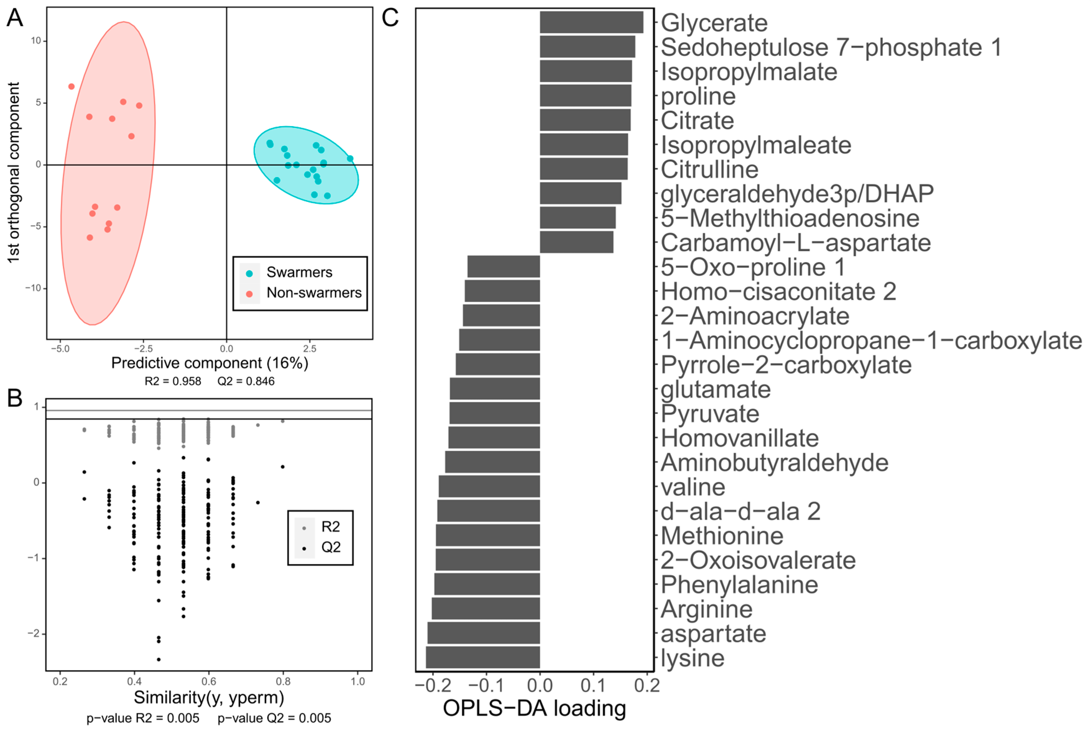
4.2.2. Supervised Multivariate Approaches

Supervised multivariate analysis methods are used to determine the strength of the correlation of the multiple variables with the phenotype of interest. Formally, univariate tests are supervised analyses, so many of the supervised multivariate analyses are univariate methods extended for multiple explanatory variables. Some examples of these methods are multiple linear regression (MLR), which is used when the phenotype to be explained is quantitative, and multiple logistic regression, used when the phenotype is categorical, with only two groups. Multinomial logistic regression can be used when there are more than two categories. For MLR, the significance of the full model can be obtained using the p-value computed from the F-statistic, while the significance of the association of each one of the variables to the response is given by its t-statistic. Regarding logistic regression methods, as in simple logistic regression, the significance of each one of the variables is given by the Z-value obtained with a Wald test [86].

MLR and logistic regression work well when the predictor variables are uncorrelated, but when some of them are correlated (multicollinearity), they fail to explain their individual effects on the response variable. In metabolomic datasets, where typically, there are a high number of predictors, and some of them are correlated because of their role in the same metabolic pathways, MLR might not be the best solution. Partial least squares methods solve this problem, being widely used in metabolomics for this reason. These methods include partial least squares (PLS), partial least squares discriminant analysis (PLS-DA), orthogonal partial least squares (OPLS) and orthogonal partial least squares discriminant analysis (OPLS-DA) [96,97]. PLS solves the multicollinearity by reducing the dimension of the data, projecting the variables to a lower dimension space that maximizes the covariance with the response variable. OPLS goes one step further by separating the variability that is correlated to the response variable and the variability that is orthogonal to it, making easier the interpretation of the influence of each individual variable on the response variable, but not improving the overall model results. PLS-DA and OPLS-DA are versions of the methods intended to work with discrete binary response variables, but their foundations are the same as the ones of their continuous counterparts. The significance of the metabolites in the separation of the samples according to the response variable can be determined using the variable importance in projection (VIP) score. This statistic is defined as the weighted sum of squares of the PLS weight, reflecting the importance of the variable to the entire model [98]. The common threshold to consider a variable significant is VIP ≥ 1 [99,100,101].

The drawback of the PLS methods is that they are prone to overfitting [102]. To solve this obstacle, a good approach is to split the dataset into training and testing subsets and to assess whether the performance in the testing set is significantly different from that in the training set. R² and Q² can be used for this aim. R², as in linear regression, indicates the proportion of the variation in the response explained by the model. Q² refers to the R² obtained with the testing set. If the model is not overfitting, R² should be high, and Q² should be slightly smaller than R², but not very different. However, because of the time-consuming nature of metabolomic sample acquisition, the number of samples is not always high enough to be able to split the dataset and still have an appropriate number of samples. An alternative to this approach is to use label permutation and cross validation [103]. In cross validation, the dataset is split into several sample subsets, the model is fitted to all the combined subsets except for one, which is tested in the left-out subset. This process is repeated until all the subsets have been used as a testing set. This allows us to have R² and Q² values while keeping all the samples for the analysis. In the permutation test, the responses variables are randomly permutated between samples. A model is then fitted to the altered dataset, and R² and Q² are computed, comparing the values to the ones of the actual model. If the model is overfitting, the permutated model might have a higher R² or Q² just by chance. Several permutation rounds are carried out, obtaining a p-value based on the proportion of R² of permutated sets higher than the actual R². Another p-value is obtained analogously for Q². Some useful graphical representations for OPLS and OPLS-DA models are a score plot of the predictive and first orthogonal components (Figure 3A), a scatterplot of the R² and Q² values obtained before and after label permutation (Figure 3B) and a bar plot of each metabolite’s loading for the predictor component (Figure 3C). These plots allow us to visualize how well the model is separating the samples, if the model is statistically significant and the contribution of each metabolite to the separation of the samples according to the response variable, respectively.

Another multivariate supervised method useful in omics analysis is random forest, which is less prone to overfitting in comparison with PLS methods [102]. A random forest is based on the decision tree method. Decision trees iteratively select the variable that best splits the data into two subsets, according to a threshold that maximizes that separation (i.e., minimize the sum of the squared residuals) [104]. At the end, the samples are separated according to similar values of the response variable. They can be used with discrete or continuous response and predictor variables (although in metabolomics, predictors will always be continuous). Decision trees that work with continuous response variables are denominated regression trees, and when the response variable is discrete, they are called classification trees [104]. Decision trees are very prone to overfitting, so random forests come as a solution to this problem [105]. In random forests, instead of fitting a single tree, an ensemble of trees is fitted to randomly generated subsets of the total samples, and a random subset of the total number of predictor variables (sample and variable bagging, respectively) is created with the aim of making each tree in the ensemble as uncorrelated to each other as possible [106,107]. The results of each tree are aggregated by either averaging (in case of regression trees) or majority vote (in the case of classification trees) to obtain the global results [108]. The resulting model can be analyzed to obtain the importance of each variable in the prediction of the outcome by permuting the values of each variable and computing how much the accuracy of the resulting model decreases [105]. Besides the improved dealing with overfitting, another important advantage of random forest is that it can deal with non-linear relationships between the groups. This contrasts with PLS methods, which try to maximize the separation along the response variable using linear combinations of the explanatory variables. While being less prone to overfitting than PLS, random forests still can overfit the data, so it is advisable to perform cross validation to assess the performance.

Linear and logistic regression models can be implemented using the glm function in R, while for Python, the scikit learn library is the best option [94]. Multinomial logistic regression can be implemented in R using the nnet R package [109], and some options for implementing the PLS methods described in this section are the ropls and pls R packages [110,111], and the scikit-learn library and pyopls module for Python [94,112]. Regarding random forests, they can be implemented in R using the caret and randomForest R packages [113,114], and in Python, with scikit-learn [94].

5. Metabolic Pathway Enrichment

Once the set of metabolites significatively associated with the biological factor(s) of interest is known, it is important to determine which are the metabolic subsystems that are more likely to be perturbed to gain biological insight. This process is known as metabolic pathway enrichment. Pathway enrichment methods, as other computational tools used in metabolomics, were inherited from transcriptomics and proteomics. The different metabolic pathway enrichment methods can be divided into three different groups: over-representation analysis (ORA), functional class scoring (FCS) and pathway topology (PT) [115].

5.1. Over-Representation Analysis (ORA)

ORA is the simplest approach for performing metabolic pathway enrichment. It relies on statistical tests that determine which metabolic pathways have more metabolites with significantly altered abundances than what could be expected by chance [116]. Among ORA’s advantages are its simplicity, the ease of implementation and its fast computation time. However, it also has several limitations, among them are that it does not account for the actual metabolite abundances and instead catalogues the metabolites as differential by applying a threshold to a determined statistic and discarding the ones that do not pass the threshold, therefore implying information loss. It also does not take into account the interactions of the metabolites within the metabolic network, which implies that alterations in any one of the metabolites within a pathway have the same effect on it. It also considers metabolic pathways as independent isolated compartments, which is not the case [115]. ORA can be easily implemented directly in any programming language with statistical capabilities such as R or Python, and it is available as prebuilt functions in R packages such as clusterProfiler [117].

5.2. Functional Class Scoring (FCS)

FCS tries to improve the information loss limitation ORA implies using the actual metabolite abundances of the whole dataset, without applying any statistic-based threshold. The hypothesis supporting this approach is that small but coordinated changes in several metabolites belonging to the same pathway can produce observable differences [115]. There are two types of FCS methods: univariate and multivariate FCS methods [118]. In univariate FCS methods, a score is computed for each individual metabolite based on the correlation with the studied biological factor, to later integrate them into a single score for each set of metabolites (metabolic pathway), while in multivariate FCS methods, the score is directly computed for each pathway [118]. The pathway scores are tested for significance using a null hypothesis either by permuting the phenotypes or the metabolites [115]. FCS methods do not solve all the ORA limitations, still considering each metabolic pathway as an independent unit and not considering the positions of metabolites within the metabolic network.

MSEA, the metabolomic version of GSEA (gene set enrichment analysis, an FCS univariate method intended to be used with transcriptomic data) [119], can be implemented in the metaboAnalyst web server and the R package version metaboAnalystR [22,120]. mPLAGE, the metabolomic-adapted version of PLAGE (pathway-level analysis of gene expression), is another FCS method that is implemented in Python within the PALS library, which is also available as a web application (https://pals.glasgowcompbio.org/app/, accessed on 15 April 2024) and as a standalone program [121,122].

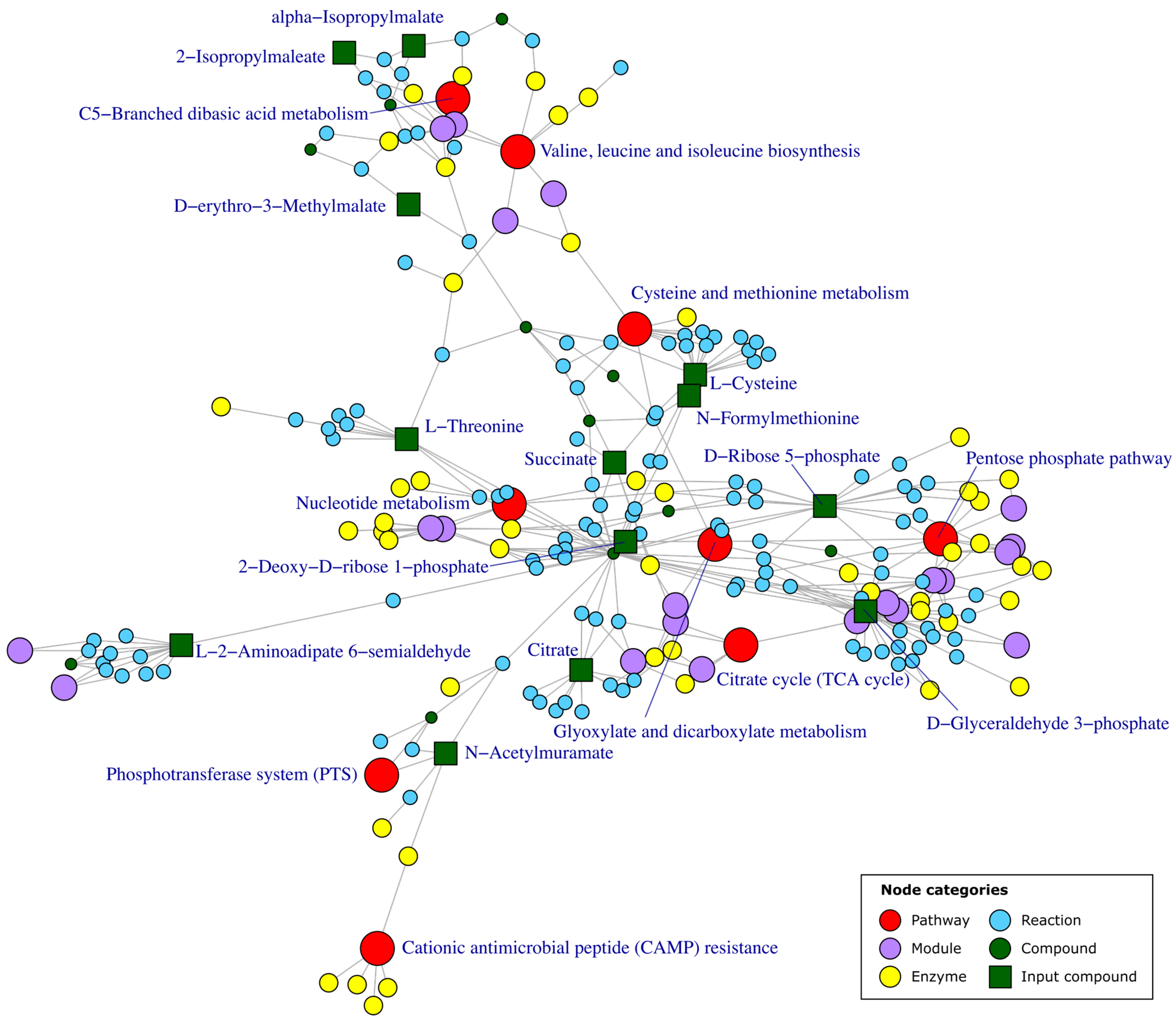
5.3. Pathway Topology (PT)

PT methods take advantage of the fact that databases such as KEGG provide information about the interactions between different elements of a metabolic network. They build a graph accounting for all the relationships and use it for determining how likely it is that differences in abundances in given metabolites affect certain metabolic pathways. There are different approaches that consider the metabolic network, each of them with its own limitations. Some examples of these methods are NetGSA, FELLA and DEGraph, which can be implemented through the netgsa, FELLA and DEGraph R packages, respectively [123,124,125,126]. NetGSA uses a graph based on the interaction between the different elements of the metabolic network, which must be provided by the user as an adjacency matrix. With this network, it calculates the influence of the concentration of each metabolite on the rest of them. It then uses this propagation to decompose the reads of the abundance of each metabolite at baseline level and propagate a signal through its neighbors. With these values, it then computes a statistic for each pathway to determine if the pathway is potentially perturbed [123]. FELLA retrieves a graph consisting of the interconnections between the different entries existing in the KEGG database for a given organism, to later apply network propagation algorithms on it using as input differentially abundant metabolites. The result is a subnetwork of entries with a high probability of receiving propagated signals from the input metabolites, meaning that they are highly interconnected [125] (Figure 4). DEGraph compares two conditions using the same interconnected graph, which can be downloaded from KEGG using the DEGraph R package. It uses a Hotelling T² test on a lower dimension space built from the graph to determine the significances of subnetworks (pathways) within the graph [126].

6. Generating Insight When Metabolomic Data Are Not Available: Genome-Scale Metabolic Models

There are some cases where the acquisition of intracellular metabolomic data is challenging, such as during the infection of animal or cellular models with intracellular pathogens like Mycobacterium tuberculosis or Legionella pneumophilla [127]. In this situation, the recovery of the bacteria from within the infected cells at sufficient biomass amounts without perturbing the metabolic state of the bacteria makes the obtention of metabolomic data virtually impossible. Genome-scale metabolic models (GEMs) are a suitable alternative for evaluating how differences in genomic content translate into distinct metabolic phenotypes. GEMs are representations of the metabolic capabilities of an organism, based on its genomic content [128]. They have been used with success to predict the growth rate of an organism in a particular medium composition, gene essentiality, the production of virulence factors and the response to stresses in different microorganisms [73,129]. GEM reconstruction typically starts with a genome annotation of the organism to be modeled, from which the reactions that the organism is capable of catalyzing are inferred. With these reactions, a draft metabolic network is automatically built, accounting for the constraints imposed by reaction stoichiometry. Later, further constraints based on experimental data are applied. They include the compartmentalization of reactions and compounds, measured intake and secretion rates of metabolic compounds, and biomass composition, integrated in a special reaction, denominated a biomass reaction, which represents the specific growth rate (h⁻¹) [130]. The obtained metabolic network will contain some gaps due to incompleteness and mistakes in the annotation and promiscuous enzymes that catalyze reactions that are not accounted for, which will need to be filled. This step is preferred to be carried out manually [131].

Once the metabolic network is complete, the rate of change in each metabolite concentration can be represented as follows:

$$\frac{dC}{dt}=Sv$$

(1)

where C is a vector of metabolite concentrations; S is the stoichiometric matrix, with each row representing a metabolite, and each column, a reaction, and the matrix elements are the stoichiometric coefficients of each metabolite relatively to each reaction (positive if the metabolite is produced, negative if it is consumed, zero if does not intervene in the reaction); and v is the vector of reaction rates or fluxes [132]. As the metabolic reactions occur at a much shorter time scale than biomass growth, the system is assumed to be in stationary state, so

$$0=Sv$$

(2)

Given that the biomass formation equation represents specific growth rate, and the substrates to form biomass are indicated in mmol/gDW (gram of dry weight), the unit of the reaction fluxes is mmol/(gDW·h). This system of equations will be under-determined, as the number of reactions is higher than the number of metabolites for known metabolic networks. So, rather than providing a single solution of reaction fluxes for a particular medium composition, the GEM will delimit a multidimensional space containing all the metabolic states that the model predicts to be possible in the specified conditions [130]. There are different approaches available for obtaining particular solutions. The first one is flux balance analysis (FBA), which consists of maximizing (or minimizing) at least one objective reaction [133]. Usually, objective reactions are the biomass and/or ATP production maximization and/or minimization of the total flux through the metabolic network [134,135]. With FBA, a flux distribution in the edge of the solution space is obtained, under the assumption that a set of objective functions is at its maximum (Figure 5A). But in some situations, this assumption might not be adequate. In many natural environments, where nutrients are not abundant, the organisms prioritize global robustness against a wider range of stresses rather than maximizing a few objectives such as energy production or growth rate [134]. One example is the M. tuberculosis macrophage infectious process, where bacteria divert several resources to counteract the stresses imposed by the host [136]. Another instance is the rhamnolipid production of Pseudomonas aeruginosa, induced by a high-density bacterial population. Here, this microorganism secretes vast amounts of carbon-rich resources to the extracellular medium instead of using them for growth [137]. Additionally, during adaptation to different temperatures, Arabidopsis thaliana prioritizes the reallocation of metabolic resources to adapt to the new conditions [138]. In such situations, flux sampling is a suitable alternative that allows researchers to examine flux distributions without introducing any bias. Flux sampling consists of taking random samples of the solution space imposed by the model’s constraints (Figure 5B). If the number of samples is large enough, it is possible to infer the shape of the solution space [139], enabling comparisons between the sampled flux distributions of model versions that reflect different genotypes or conditions [127].

In employing GEMs and FBA and/or flux sampling, a flux matrix can be obtained for different genotypes or conditions. This matrix resembles the imputed and normalized metabolite matrix obtained in Section 3. The statistical analyses and the pathway enrichment methods discussed in Section 4 and Section 5 can be used to determine, for example, which are the metabolic pathways more likely to be affected by genomic differences between different bacterial strains when intracellular metabolome data are not available [127].

7. Conclusions

Metabolomics is a field with promising prospects across several life science disciplines [140]. As a relatively new field compared to other omics, metabolomics lacks a standardized procedure for handling derived data analysis. In this review, we compiled the most commonly applied approaches and proposed a typical metabolomic bioinformatic workflow starting from raw data acquisition, whether with LC-MS, GC-MS or NMR. We divided the process into four modules: raw spectrum preprocessing, raw peak area preprocessing, statistical analysis and metabolic pathway enrichment. For each step, we highlighted some of the most popular approaches and indicated state-of-the-art tools that readers can use. We diagrammed the workflow in Figure 6. This guide aims to navigate the challenges that might arise in each step of bioinformatic analysis and emphasize the advantages and drawbacks of the presented methods. As an alternative to acquiring intracellular metabolomics data when it is not possible, we proposed using GEMs to generate metabolomic-like data. This data can help determine how genomic differences translate into metabolic discrepancies, considering the entire metabolic network [127]. If intracellular metabolomic data are not available but it is possible to measure the exchange rates of extracellular metabolites, it is possible to further constrain these models. This allows us to infer the metabolic phenotype across various environmental conditions or individuals of the same species [138,141]. The emergence of single-cell transcriptomic technologies enables the building of context-specific GEMs with cell-type resolution, opening up numerous avenues for new research areas [142].

References

1. Oliver, S.G.; Winson, M.K.; Kell, D.B.; Baganz, F. Systematic Functional Analysis of the Yeast Genome. Trends Biotechnol. 1998, 16, 373–378. [Google Scholar] [CrossRef] [PubMed]
2. Fiehn, O. Metabolomics—The Link between Genotypes and Phenotypes. Plant Mol. Biol. 2002, 48, 155–171. [Google Scholar] [CrossRef] [PubMed]
3. Marian, A.J. Molecular Genetic Studies of Complex Phenotypes. Transl. Res. 2012, 159, 64–79. [Google Scholar] [CrossRef] [PubMed]
4. Zulianello, L.; Canard, C.; Köhler, T.; Caille, D.; Lacroix, J.S.; Meda, P. Rhamnolipids Are Virulence Factors That Promote Early Infiltration of Primary Human Airway Epithelia by Pseudomonas aeruginosa. Infect. Immun. 2006, 74, 3134–3147. [Google Scholar] [CrossRef] [PubMed]
5. Davey, M.E.; Caiazza, N.C.; O’Toole, G.A. Rhamnolipid Surfactant Production Affects Biofilm Architecture in Pseudomonas aeruginosa PAO1. J. Bacteriol. 2003, 185, 1027–1036. [Google Scholar] [CrossRef] [PubMed]
6. Caiazza, N.C.; Shanks, R.M.Q.; O’Toole, G.A. Rhamnolipids Modulate Swarming Motility Patterns of Pseudomonas aeruginosa. J. Bacteriol. 2005, 187, 7351–7361. [Google Scholar] [CrossRef] [PubMed]
7. Sabra, W.; Kim, E.J.; Zeng, A.P. Physiological Responses of Pseudomonas aeruginosa PAO1 to Oxidative Stress in Controlled Microaerobic and Aerobic Cultures. Microbiology 2002, 148, 3195–3202. [Google Scholar] [CrossRef] [PubMed]
8. Mukhopadhyay, S.; Nair, S.; Ghosh, S. Pathogenesis in Tuberculosis: Transcriptomic Approaches to Unraveling Virulence Mechanisms and Finding New Drug Targets. FEMS Microbiol. Rev. 2012, 36, 463–485. [Google Scholar] [CrossRef] [PubMed]
9. Galagan, J.E.; Minch, K.; Peterson, M.; Lyubetskaya, A.; Azizi, E.; Sweet, L.; Gomes, A.; Rustad, T.; Dolganov, G.; Glotova, I.; et al. The Mycobacterium tuberculosis Regulatory Network and Hypoxia. Nature 2013, 499, 178–183. [Google Scholar] [CrossRef]
10. Raghunandanan, S.; Jose, L.; Gopinath, V.; Kumar, R.A. Comparative Label-Free Lipidomic Analysis of Mycobacterium tuberculosis during Dormancy and Reactivation. Sci. Rep. 2019, 9, 3660. [Google Scholar] [CrossRef]
11. Ye, D.; Li, X.; Shen, J.; Xia, X. Microbial Metabolomics: From Novel Technologies to Diversified Applications. TrAC-Trends Anal. Chem. 2022, 148, 116540. [Google Scholar] [CrossRef]
12. Emwas, A.H.; Roy, R.; McKay, R.T.; Tenori, L.; Saccenti, E.; Nagana Gowda, G.A.; Raftery, D.; Alahmari, F.; Jaremko, L.; Jaremko, M.; et al. Nmr Spectroscopy for Metabolomics Research. Metabolites 2019, 9, 123. [Google Scholar] [CrossRef] [PubMed]
13. Lu, H.; Liang, Y.; Dunn, W.B.; Shen, H.; Kell, D.B. Comparative Evaluation of Software for Deconvolution of Metabolomics Data Based on GC-TOF-MS. TrAC-Trends Anal. Chem. 2008, 27, 215–227. [Google Scholar] [CrossRef]
14. Fiehn, O. Metabolomics by Gas Chromatography-Mass Spectrometry: The Combination of Targeted and Untargeted Profiling. Curr. Protoc. Mol. Biol. 2017, 114, 30.4.1–30.4.32. [Google Scholar] [CrossRef] [PubMed]
15. Perez, E.R.; Knapp, J.A.; Horn, C.K.; Stillman, S.L.; Evans, J.E.; Arfsten, D.P. Comparison of LC-MS-MS and GC-MS Analysis of Benzodiazepine Compounds Included in the Drug Demand Reduction Urinalysis Program. J. Anal. Toxicol. 2016, 40, 201–207. [Google Scholar] [CrossRef] [PubMed]
16. Chen, C.; Gonzalez, F.J.; Idle, J.R. LC-MS-Based Metabolomics in Drug Metabolism. Drug Metab. Rev. 2007, 39, 581–597. [Google Scholar] [CrossRef]
17. Johnson, C.H.; Ivanisevic, J.; Benton, H.P.; Siuzdak, G. Bioinformatics: The next Frontier of Metabolomics. Anal. Chem. 2015, 87, 147–156. [Google Scholar] [CrossRef] [PubMed]
18. Emwas, A.H.M. The Strengths and Weaknesses of NMR Spectroscopy and Mass Spectrometry with Particular Focus on Metabolomics Research. In Metabonomics: Methods and Protocols; Bjerrum, J.T., Ed.; Humana Press: New York, NY, USA, 2015; Volume 1277, pp. 161–194. [Google Scholar]
19. Edison, A.S.; Colonna, M.; Gouveia, G.J.; Holderman, N.R.; Judge, M.T.; Shen, X.; Zhang, S. NMR: Unique Strengths That Enhance Modern Metabolomics Research. Anal. Chem. 2021, 93, 478–499. [Google Scholar] [CrossRef] [PubMed]
20. Karaman, I.; Climaco Pinto, R.; Graça, G. Chapter 8—Metabolomics Data Preprocessing: From Raw Data to Features for Statistical Analysis. In Comprehensive Analytical Chemistry; Jaumot, J., Bedia, C., Tauler, R., Eds.; Elsevier: Amsterdam, The Netherlands, 2018; Volume 82, ISBN 9780444640444. [Google Scholar]
21. Alonso, A.; Marsal, S.; Julià, A. Analytical Methods in Untargeted Metabolomics: State of the Art in 2015. Front. Bioeng. Biotechnol. 2015, 3, 23. [Google Scholar] [CrossRef]
22. Pang, Z.; Chong, J.; Zhou, G.; De Lima Morais, D.A.; Chang, L.; Barrette, M.; Gauthier, C.; Jacques, P.É.; Li, S.; Xia, J. MetaboAnalyst 5.0: Narrowing the Gap between Raw Spectra and Functional Insights. Nucleic Acids Res. 2021, 49, W388–W396. [Google Scholar] [CrossRef]
23. Delaglio, F.; Grzesiek, S.; Vuister, G.W.; Zhu, G.; Pfeifer, J.; Bax, A. NMRPipe: A Multidimensional Spectral Processing System Based on UNIX Pipes. J. Biomol. NMR 1995, 6, 277–293. [Google Scholar] [CrossRef] [PubMed]
24. van Beek, J.D. MatNMR: A Flexible Toolbox for Processing, Analyzing and Visualizing Magnetic Resonance Data in Matlab®. J. Magn. Reson. 2007, 187, 19–26. [Google Scholar] [CrossRef] [PubMed]
25. Chong, J.; Yamamoto, M.; Xia, J. MetaboAnalystR 2.0: From Raw Spectra to Biological Insights. Metabolites 2019, 9, 57. [Google Scholar] [CrossRef] [PubMed]
26. Smith, C.A.; Want, E.J.; O’Maille, G.; Abagyan, R.; Siuzdak, G. XCMS: Processing Mass Spectrometry Data for Metabolite Profiling Using Nonlinear Peak Alignment, Matching, and Identification. Anal. Chem. 2006, 78, 779–787. [Google Scholar] [CrossRef]
27. Altenhof, A.R.; Mason, H.; Schurko, R.W. DESPERATE: A Python Library for Processing and Denoising NMR Spectra. J. Magn. Reson. 2023, 346, 107320. [Google Scholar] [CrossRef]
28. Qiu, T.; Wang, Z.; Liu, H.; Guo, D.; Qu, X. Review and Prospect: NMR Spectroscopy Denoising and Reconstruction with Low-Rank Hankel Matrices and Tensors. Magn. Reson. Chem. 2020, 59, 324–345. [Google Scholar] [CrossRef] [PubMed]
29. Bauer, C.; Cramer, R.; Schuchhardt, J. Evaluation of Peak-Picking Algorithms for Protein Mass Spectrometry. In Data Mining in Proteomics: From Standards to Applications. Methods in Molecular Biology; Humana Press: Totowa, NJ, USA, 2011; Volume 696, pp. 341–352. ISBN 9781607619871. [Google Scholar]
30. Liu, Z.; Abbas, A.; Jing, B.Y.; Gao, X. WaVPeak: Picking NMR Peaks through Wavelet-Based Smoothing and Volume-Based Filtering. Bioinformatics 2012, 28, 914–920. [Google Scholar] [CrossRef] [PubMed]
31. Xia, J.; Psychogios, N.; Young, N.; Wishart, D.S. MetaboAnalyst: A Web Server for Metabolomic Data Analysis and Interpretation. Nucleic Acids Res. 2009, 37, W652–W660. [Google Scholar] [CrossRef] [PubMed]
32. Xi, Y.; Rocke, D.M. Baseline Correction for NMR Spectroscopic Metabolomics Data Analysis. BMC Bioinform. 2008, 9, 324. [Google Scholar] [CrossRef]
33. Li, D.W.; Hansen, A.L.; Yuan, C.; Bruschweiler-Li, L.; Brüschweiler, R. DEEP Picker Is a Deep Neural Network for Accurate Deconvolution of Complex Two-Dimensional NMR Spectra. Nat. Commun. 2021, 12, 5229. [Google Scholar] [CrossRef]
34. Bueschl, C.; Doppler, M.; Varga, E.; Seidl, B.; Flasch, M.; Warth, B.; Zanghellini, J. PeakBot: Machine-Learning-Based Chromatographic Peak Picking. Bioinformatics 2022, 38, 3422–3428. [Google Scholar] [CrossRef] [PubMed]
35. Tomasi, G.; Van Den Berg, F.; Andersson, C. Correlation Optimized Warping and Dynamic Time Warping as Preprocessing Methods for Chromatographic Data. J. Chemom. 2004, 18, 231–241. [Google Scholar] [CrossRef]
36. Nielsen, N.P.V.; Carstensen, J.M.; Smedsgaard, J. Aligning of Single and Multiple Wavelength Chromatographic Profiles for Chemometric Data Analysis Using Correlation Optimised Warping. J. Chromatogr. A 1998, 805, 17–35. [Google Scholar] [CrossRef]
37. Vu, T.N.; Laukens, K. Getting Your Peaks in Line: A Review of Alignment Methods for NMR Spectral Data. Metabolites 2013, 3, 259–276. [Google Scholar] [CrossRef] [PubMed]
38. Wishart, D.S.; Guo, A.C.; Oler, E.; Wang, F.; Anjum, A.; Peters, H.; Dizon, R.; Sayeeda, Z.; Tian, S.; Lee, B.L.; et al. HMDB 5.0: The Human Metabolome Database for 2022. Nucleic Acids Res. 2022, 50, D622–D631. [Google Scholar] [CrossRef] [PubMed]
39. Xue, J.; Guijas, C.; Benton, H.P.; Warth, B.; Siuzdak, G. METLIN MS2 Molecular Standards Database: A Broad Chemical and Biological Resource. Nat. Methods 2020, 17, 953–954. [Google Scholar] [CrossRef] [PubMed]
40. Mamede, L.; Fall, F.; Schoumacher, M.; Ledoux, A.; De Tullio, P.; Govaerts, B.; Fr, M. Comparison of Extraction Methods in Vitro Plasmodium falciparum: A 1H NMR and LC-MS Joined Approach. Biochem. Biophys. Res. Commun. 2024, 703, 149684. [Google Scholar] [CrossRef] [PubMed]
41. Hrydziuszko, O.; Viant, M.R. Missing Values in Mass Spectrometry Based Metabolomics: An Undervalued Step in the Data Processing Pipeline. Metabolomics 2012, 8, S161–S174. [Google Scholar] [CrossRef]
42. Barnard, J.; Meng, X.L. Applications of Multiple Imputation in Medical Studies: From AIDS to NHANES. Stat. Methods Med. Res. 1999, 8, 17–36. [Google Scholar] [CrossRef]
43. Bijlsma, S.; Bobeldijk, I.; Verheij, E.R.; Ramaker, R.; Kochhar, S.; Macdonald, I.A.; Van Ommen, B.; Smilde, A.K. Large-Scale Human Metabolomics Studies: A Strategy for Data (Pre-) Processing and Validation. Anal. Chem. 2006, 78, 567–574. [Google Scholar] [CrossRef]
44. Kokla, M.; Virtanen, J.; Kolehmainen, M.; Paananen, J.; Hanhineva, K. Random Forest-Based Imputation Outperforms Other Methods for Imputing LC-MS Metabolomics Data: A Comparative Study. BMC Bioinform. 2019, 20, 492. [Google Scholar] [CrossRef]
45. Hong, S.; Lynn, H.S. Accuracy of Random-Forest-Based Imputation of Missing Data in the Presence of Non-Normality, Non-Linearity, and Interaction. BMC Med. Res. Methodol. 2020, 20, 99. [Google Scholar] [CrossRef]
46. Hu, L.Y.; Huang, M.W.; Ke, S.W.; Tsai, C.F. The Distance Function Effect on K-Nearest Neighbor Classification for Medical Datasets. Springerplus 2016, 5, 1304. [Google Scholar] [CrossRef]
47. Kim, H.; Golub, G.H.; Park, H. Missing Value Estimation for DNA Microarray Gene Expression Data: Local Least Squares Imputation. Bioinformatics 2005, 21, 187–198. [Google Scholar] [CrossRef] [PubMed]
48. Troyanskaya, O.; Cantor, M.; Sherlock, G.; Brown, P.; Hastie, T.; Tibshirani, R.; Botstein, D.; Altman, R.B. Missing Value Estimation Methods for DNA Microarrays. Bioinformatics 2001, 17, 520–525. [Google Scholar] [CrossRef]
49. Oba, S.; Sato, M.A.; Takemasa, I.; Monden, M.; Matsubara, K.I.; Ishii, S. A Bayesian Missing Value Estimation Method for Gene Expression Profile Data. Bioinformatics 2003, 19, 2088–2096. [Google Scholar] [CrossRef]
50. Ilin, A.; Raiko, T. Practical Approaches to Principal Component Analysis in the Presence of Missing Values. J. Mach. Learn. Res. 2010, 11, 1957–2000. [Google Scholar]
51. Leek, J.T.; Scharpf, R.B.; Bravo, H.C.; Simcha, D.; Langmead, B.; Johnson, W.E.; Geman, D.; Baggerly, K.; Irizarry, R.A. Tackling the Widespread and Critical Impact of Batch Effects in High-Throughput Data. Nat. Rev. Genet. 2010, 11, 733–739. [Google Scholar] [CrossRef] [PubMed]
52. Marioni, J.C.; Mason, C.E.; Mane, S.M.; Stephens, M.; Gilad, Y. RNA-Seq: An Assessment of Technical Reproducibility and Comparison with Gene Expression Arrays. Genome Res. 2008, 18, 1509–1517. [Google Scholar] [CrossRef]
53. Karpievitch, Y.V.; Dabney, A.R.; Smith, R.D. Normalization and Missing Value Imputation for Label-Free LC-MS Analysis. BMC Bioinform. 2012, 13, S5. [Google Scholar] [CrossRef]
54. Vandesompele, J.; De Preter, K.; Pattyn, F.; Poppe, B.; Van Roy, N.; De Paepe, A.; Speleman, F. Accurate Normalization of Real-Time Quantitative RT-PCR Data by Geometric Averaging of Multiple Internal Control Genes. Rock. Mech. Rock. Eng. 2002, 3, research0034.1. [Google Scholar] [CrossRef] [PubMed]
55. Wiśniewski, J.R.; Mann, M. A Proteomics Approach to the Protein Normalization Problem: Selection of Unvarying Proteins for MS-Based Proteomics and Western Blotting. J. Proteome Res. 2016, 15, 2321–2326. [Google Scholar] [CrossRef] [PubMed]
56. Wu, Y.; Li, L. Sample Normalization Methods in Quantitative Metabolomics. J. Chromatogr. A 2016, 1430, 80–95. [Google Scholar] [CrossRef] [PubMed]
57. Chen, J.; Zhang, P.; Lv, M.; Guo, H.; Huang, Y.; Zhang, Z.; Xu, F. Influences of Normalization Method on Biomarker Discovery in Gas Chromatography-Mass Spectrometry-Based Untargeted Metabolomics: What Should Be Considered? Anal. Chem. 2017, 89, 5342–5348. [Google Scholar] [CrossRef]
58. Temmerman, L.; De Livera, A.M.; Browne, J.B.; Sheedy, J.R.; Callahan, D.L.; Nahid, A.; De Souza, D.P.; Schoofs, L.; Tull, D.L.; McConville, M.J.; et al. Cross-Platform Urine Metabolomics of Experimental Hyperglycemia in Type 2 Diabetes. J. Diabetes Metab. 2012, 6, 1–7. [Google Scholar] [CrossRef]
59. De Livera, A.M.; Sysi-Aho, M.; Jacob, L.; Gagnon-Bartsch, J.A.; Castillo, S.; Simpson, J.A.; Speed, T.P. Statistical Methods for Handling Unwanted Variation in Metabolomics Data. Anal. Chem. 2015, 87, 3606–3615. [Google Scholar] [CrossRef] [PubMed]
60. Edmands, W.M.B.; Ferrari, P.; Scalbert, A. Normalization to Specific Gravity Prior to Analysis Improves Information Recovery from High Resolution Mass Spectrometry Metabolomic Profiles of Human Urine. Anal. Chem. 2014, 86, 10925–10931. [Google Scholar] [CrossRef]
61. Marcinowska, R.; Trygg, J.; Wolf-Watz, H.; Mortiz, T.; Surowiec, I. Optimization of a Sample Preparation Method for the Metabolomic Analysis of Clinically Relevant Bacteria. J. Microbiol. Methods 2011, 87, 24–31. [Google Scholar] [CrossRef] [PubMed]
62. Chen, Y.; Shen, G.; Zhang, R.; He, J.; Zhang, Y.; Xu, J.; Yang, W.; Chen, X.; Song, Y.; Abliz, Z. Combination of Injection Volume Calibration by Creatinine and MS Signals’ Normalization to Overcome Urine Variability in LC-MS-Based Metabolomics Studies. Anal. Chem. 2013, 85, 7659–7665. [Google Scholar] [CrossRef]
63. De Livera, A.M.; Dias, D.A.; De Souza, D.; Rupasinghe, T.; Pyke, J.; Tull, D.; Roessner, U.; McConville, M.; Speed, T.P. Normalizing and Integrating Metabolomics Data. Anal. Chem. 2012, 84, 10768–10776. [Google Scholar] [CrossRef]
64. Antonelli, J.; Claggett, B.L.; Henglin, M.; Kim, A.; Ovsak, G.; Kim, N.; Deng, K.; Rao, K.; Tyagi, O.; Watrous, J.D.; et al. Statistical Workflow for Feature Selection in Human Metabolomics Data. Metabolites 2019, 9, 143. [Google Scholar] [CrossRef]
65. van den Berg, R.A.; Hoefsloot, H.C.J.; Westerhuis, J.A.; Smilde, A.K.; van der Werf, M.J. Centering, Scaling, and Transformations: Improving the Biological Information Content of Metabolomics Data. BMC Genom. 2006, 7, 142. [Google Scholar] [CrossRef]
66. De Livera, A.M.; Olshansky, G.; Simpson, J.A.; Creek, D.J. NormalizeMets: Assessing, Selecting and Implementing Statistical Methods for Normalizing Metabolomics Data. Metabolomics 2018, 14, 54. [Google Scholar] [CrossRef]
67. Sysi-Aho, M.; Katajamaa, M.; Yetukuri, L.; Orešič, M. Normalization Method for Metabolomics Data Using Optimal Selection of Multiple Internal Standards. BMC Bioinform. 2007, 8, 93. [Google Scholar] [CrossRef] [PubMed]
68. Grocholska, P.; Bachor, R. Trends in the Hydrogen−deuterium Exchange at the Carbon Centers. Preparation of Internal Standards for Quantitative Analysis by Lc-Ms. Molecules 2021, 26, 2989. [Google Scholar] [CrossRef] [PubMed]
69. Gullberg, J.; Jonsson, P.; Nordström, A.; Sjöström, M.; Moritz, T. Design of Experiments: An Efficient Strategy to Identify Factors Influencing Extraction and Derivatization of Arabidopsis thaliana Samples in Metabolomic Studies with Gas Chromatography/Mass Spectrometry. Anal. Biochem. 2004, 331, 283–295. [Google Scholar] [CrossRef]
70. Liu, R.H.; Lin, D.L.; Chang, W.-T.; Liu, C.; Tsay, W.-I.; Li, J.-H.; Kuo, T.-L. Isotopically Labeled Analogues for Drug Quantitation. Anal. Chem. 2002, 74, 618A–626A. [Google Scholar] [CrossRef] [PubMed]
71. Redestig, H.; Fukushima, A.; Stenlund, H.; Moritz, T.; Arita, M.; Saito, K.; Kusano, M. Compensation for Systematic Cross-Contribution Improves Normalization of Mass Spectrometry Based Metabolomics Data. Anal. Chem. 2009, 81, 7974–7980. [Google Scholar] [CrossRef]
72. Gagnon-Bartsch, J.A.; Speed, T.P. Using Control Genes to Correct for Unwanted Variation in Microarray Data. Biostatistics 2012, 13, 539–552. [Google Scholar] [CrossRef]
73. Santamaria, G.; Liao, C.; Lindberg, C.; Chen, Y.; Wang, Z.; Rhee, K.; Pinto, F.; Yan, J.; Xavier, J.B. Evolution and Regulation of Microbial Secondary Metabolism. eLife 2022, 11, e76119. [Google Scholar] [CrossRef]
74. Dunn, W.B.; Broadhurst, D.; Begley, P.; Zelena, E.; Francis-Mcintyre, S.; Anderson, N.; Brown, M.; Knowles, J.D.; Halsall, A.; Haselden, J.N.; et al. Procedures for Large-Scale Metabolic Profiling of Serum and Plasma Using Gas Chromatography and Liquid Chromatography Coupled to Mass Spectrometry. Nat. Protoc. 2011, 6, 1060–1083. [Google Scholar] [CrossRef] [PubMed]
75. Sangster, T.; Major, H.; Plumb, R.; Wilson, A.J.; Wilson, I.D. A Pragmatic and Readily Implemented Quality Control Strategy for HPLC-MS and GC-MS-Based Metabonomic Analysis. Analyst 2006, 131, 1075–1078. [Google Scholar] [CrossRef] [PubMed]
76. Gika, H.G.; Theodoridis, G.A.; Wingate, J.E.; Wilson, I.D. Within-Day Reproducibility of an HPLC-MS-Based Method for Metabonomic Analysis: Application to Human Urine. J. Proteome Res. 2007, 6, 3291–3303. [Google Scholar] [CrossRef] [PubMed]
77. Broadhurst, D.; Goodacre, R.; Reinke, S.N.; Kuligowski, J.; Wilson, I.D.; Lewis, M.R.; Dunn, W.B. Guidelines and Considerations for the Use of System Suitability and Quality Control Samples in Mass Spectrometry Assays Applied in Untargeted Clinical Metabolomic Studies. Metabolomics 2018, 14, 72. [Google Scholar] [CrossRef]
78. Schiffman, C.; Petrick, L.; Perttula, K.; Yano, Y.; Carlsson, H.; Whitehead, T.; Metayer, C.; Hayes, J.; Rappaport, S.; Dudoit, S. Filtering Procedures for Untargeted Lc-Ms Metabolomics Data. BMC Bioinform. 2019, 20, 334. [Google Scholar] [CrossRef] [PubMed]
79. Begley, P.; Francis-McIntyre, S.; Dunn, W.B.; Broadhurst, D.I.; Halsall, A.; Tseng, A.; Knowles, J.; HUSERMET Consortium; Goodacre, R.; Kell, D.B. Development and Performance of a Gas Chromatography-Time-of-Flight Mass Spectrometry Analysis for Large-Scale Nontargeted Metabolomic Studies of Human Serum. Anal. Chem. 2009, 81, 7038–7046. [Google Scholar] [CrossRef]
80. Zelena, E.; Dunn, W.B.; Broadhurst, D.; Francis-McIntyre, S.; Carroll, K.M.; Begley, P.; O’Hagan, S.; Knowles, J.D.; Halsall, A.; HUSERMET Consortium; et al. Development of a Robust and Repeatable UPLC-MS Method for the Long-Term Metabolomic Study of Human Serum. Anal. Chem. 2009, 81, 1357–1364. [Google Scholar] [CrossRef]
81. Rousseeuw, P.J. Silhouettes: A Graphical Aid to the Interpretation and Validation of Cluster Analysis. J. Comput. Appl. Math. 1987, 20, 53–65. [Google Scholar] [CrossRef]
82. De Livera, A.M.; Olshansky, M.; Speed, T.P. Statistical Analysis of Metabolomics Data. In Metabolomics Tools for Natural Product Discovery; Humana Press: Totowa, NJ, USA, 2013; pp. 291–307. [Google Scholar]
83. Virtanen, P.; Gommers, R.; Oliphant, T.E.; Haberland, M.; Reddy, T.; Cournapeau, D.; Burovski, E.; Peterson, P.; Weckesser, W.; Bright, J.; et al. Author Correction: SciPy 1.0: Fundamental Algorithms for Scientific Computing in Python. Nat. Methods 2020, 17, 352. [Google Scholar] [CrossRef]
84. Hunter, J.D. Matplotlib: A 2D Graphics Environment. Comput. Sci. Eng. 2007, 9, 90–95. [Google Scholar] [CrossRef]
85. Sokal, R.R.; Rohlf, F.J. Biometry. The Principles and Practice of Statistics in Biological Research, 3rd ed.; W. H. Freeman and Company: New York, NY, USA, 1995. [Google Scholar]
86. Bewick, V.; Cheek, L.; Ball, J. Statistics Review 14: Logistic Regression. Crit. Care 2005, 9, 112–118. [Google Scholar] [CrossRef] [PubMed]
87. Broadhurst, D.I.; Kell, D.B. Statistical Strategies for Avoiding False Discoveries in Metabolomics and Related Experiments. Metabolomics 2006, 2, 171–196. [Google Scholar] [CrossRef]
88. Saccenti, E.; Hoefsloot, H.C.J.; Smilde, A.K.; Westerhuis, J.A.; Hendriks, M.M.W.B. Reflections on Univariate and Multivariate Analysis of Metabolomics Data. Metabolomics 2014, 10, 361–374. [Google Scholar] [CrossRef]
89. Worley, B.; Powers, R. Multivariate Analysis in Metabolomics. Curr. Metabolomics 2013, 1, 92–107. [Google Scholar] [CrossRef] [PubMed]
90. Şenbabaoğlu, Y.; Michailidis, G.; Li, J.Z. Critical Limitations of Consensus Clustering in Class Discovery. Sci. Rep. 2014, 4, 6207. [Google Scholar] [CrossRef]
91. John, C.R.; David, W.; Russ, D.; Goldmann, K.; Ehrenstein, M.; Pitzalis, C.; Lewis, M.; Barnes, M. M3C: Monte Carlo Reference-Based Consensus Clustering. Sci. Rep. 2020, 10, 1816. [Google Scholar] [CrossRef] [PubMed]
92. Boyle, K.E.; Monaco, H.T.; Deforet, M.; Yan, J.; Wang, Z.; Rhee, K.; Xavier, J.B. Metabolism and the Evolution of Social Behavior. Mol. Biol. Evol. 2017, 34, 2367–2379. [Google Scholar] [CrossRef]
93. van der Maaten, L.; Hinton, G. Visualizing Data Using T-SNE. J. Mach. Learn. Res. 2008, 219, 2579–2605. [Google Scholar]
94. Pedregosa, F.; Varoquaux, G.; Gramfort, A.; Michel, V.; Thirion, B.; Grisel, O.; Blondel, M.; Prettenhofer, P.; Weiss, R.; Dubourg, V.; et al. Scikit-Learn: Machine Learning in Python. J. Mach. Learn. Res. 2011, 12, 2825–2830. [Google Scholar] [CrossRef]
95. Wilkerson, M.D.; Hayes, D.N. ConsensusClusterPlus: A Class Discovery Tool with Confidence Assessments and Item Tracking. Bioinformatics 2010, 26, 1572–1573. [Google Scholar] [CrossRef]
96. Wold, S.; Sjöström, M.; Eriksson, L. PLS-Regression: A Basic Tool of Chemometrics. Chemom. Intell. Lab. Syst. 2001, 58, 109–130. [Google Scholar] [CrossRef]
97. Trygg, J.; Wold, S. Orthogonal Projections to Latent Structures (O-PLS). J. Chemom. 2002, 16, 119–128. [Google Scholar] [CrossRef]
98. Mehmood, T.; Liland, K.H.; Snipen, L.; Sæbø, S. A Review of Variable Selection Methods in Partial Least Squares Regression. Chemom. Intell. Lab. Syst. 2012, 118, 62–69. [Google Scholar] [CrossRef]
99. Rizvi, A.; Shankar, A.; Chatterjee, A.; More, T.H.; Bose, T.; Dutta, A.; Balakrishnan, K.; Madugulla, L.; Rapole, S.; Mande, S.S.; et al. Rewiring of Metabolic Network in Mycobacterium tuberculosis during Adaptation to Different Stresses. Front. Microbiol. 2019, 10, 2417. [Google Scholar] [CrossRef] [PubMed]
100. Feng, Q.; Liu, Z.; Zhong, S.; Li, R.; Xia, H.; Jie, Z.; Wen, B.; Chen, X.; Yan, W.; Fan, Y.; et al. Integrated Metabolomics and Metagenomics Analysis of Plasma and Urine Identified Microbial Metabolites Associated with Coronary Heart Disease. Sci. Rep. 2016, 6, 22525. [Google Scholar] [CrossRef] [PubMed]
101. Ma, X.; Chi, Y.H.; Niu, M.; Zhu, Y.; Zhao, Y.L.; Chen, Z.; Wang, J.B.; Zhang, C.E.; Li, J.Y.; Wang, L.F.; et al. Metabolomics Coupled with Multivariate Data and Pathway Analysis on Potential Biomarkers in Cholestasis and Intervention Effect of Paeonia lactiflora Pall. Front. Pharmacol. 2016, 7, 14. [Google Scholar] [CrossRef] [PubMed]
102. O’Boyle, N.M.; Palmer, D.S.; Nigsch, F.; Mitchell, J.B. Simultaneous Feature Selection and Parameter Optimisation Using an Artificial Ant Colony: Case Study of Melting Point Prediction. Chem. Cent. J. 2008, 2, 21. [Google Scholar] [CrossRef] [PubMed]
103. Szymańska, E.; Saccenti, E.; Smilde, A.K.; Westerhuis, J.A. Double-Check: Validation of Diagnostic Statistics for PLS-DA Models in Metabolomics Studies. Metabolomics 2012, 8, 3–16. [Google Scholar] [CrossRef]
104. Breiman, L.; Friedman, J.H.; Olshen, R.A.; Stone, C.J. Classification and Regression Trees; Chapman & Hall: London, UK; CRC: Boca Raton, FL, USA, 1984; ISBN 0412048418. [Google Scholar]
105. Breiman, L. Random Forests. Mach. Learn. 2001, 45, 5–32. [Google Scholar] [CrossRef]
106. Breiman, L. Bagging Predictors. Mach. Learn. 1996, 24, 123–140. [Google Scholar] [CrossRef]
107. Amit, Y.; Geman, D. Shape Quantization and Recognition with Randomized Trees. Neural Comput. 1997, 9, 1545–1588. [Google Scholar] [CrossRef]
108. Devroye, L.; Lugosi, G. Consistency of Random Forests and Other Averaging Classifiers. J. Mach. Learn. Res. 2008, 9, 2015–2033. [Google Scholar]
109. Venables, W.N.; Ripley, B.D. Modern Applied Statistics with S, 4th ed.; Springer: New York, NY, USA, 2002. [Google Scholar]
110. Thévenot, E.A.; Roux, A.; Xu, Y.; Ezan, E.; Junot, C. Analysis of the Human Adult Urinary Metabolome Variations with Age, Body Mass Index, and Gender by Implementing a Comprehensive Workflow for Univariate and OPLS Statistical Analyses. J. Proteome Res. 2015, 14, 3322–3335. [Google Scholar] [CrossRef] [PubMed]
111. Mevik, B.-H.; Wehrens, R. The Pls Package: Principal Component and Partial Least Squares Regression in R. J. Stat. Softw. 2007, 18. [Google Scholar] [CrossRef]
112. BiRG—Wright State University Pyopls. Available online: https://pypi.org/project/pyopls/ (accessed on 15 April 2024).
113. Kuhn, M. Building Predictive Models in R Using the Caret Package. J. Stat. Softw. 2008, 28, 1–26. [Google Scholar] [CrossRef]
114. Liaw, A.; Wiener, M. Classification and Regression by RandomForest. R News 2002, 2, 18–22. [Google Scholar] [CrossRef]
115. Khatri, P.; Sirota, M.; Butte, A.J. Ten Years of Pathway Analysis: Current Approaches and Outstanding Challenges. PLoS Comput. Biol. 2012, 8, e1002375. [Google Scholar] [CrossRef]
116. Goeman, J.J.; Bühlmann, P. Analyzing Gene Expression Data in Terms of Gene Sets: Methodological Issues. Bioinformatics 2007, 23, 980–987. [Google Scholar] [CrossRef] [PubMed]
117. Yu, G.; Wang, L.G.; Han, Y.; He, Q.Y. ClusterProfiler: An R Package for Comparing Biological Themes among Gene Clusters. Omics J. Integr. Biol. 2012, 16, 284–287. [Google Scholar] [CrossRef]
118. Maleki, F.; Ovens, K.; Hogan, D.J.; Kusalik, A.J. Gene Set Analysis: Challenges, Opportunities, and Future Research. Front. Genet. 2020, 11, 654. [Google Scholar] [CrossRef]
119. Mootha, V.K.; Lindgren, C.M.; Eriksson, K.F.; Subramanian, A.; Sihag, S.; Lehar, J.; Puigserver, P.; Carlsson, E.; Ridderstråle, M.; Laurila, E.; et al. PGC-1α-Responsive Genes Involved in Oxidative Phosphorylation Are Coordinately Downregulated in Human Diabetes. Nat. Genet. 2003, 34, 267–273. [Google Scholar] [CrossRef]
120. Pang, Z.; Chong, J.; Li, S.; Xia, J. MetaboAnalystR 3.0: Toward an Optimized Workflow for Global Metabolomics. Metabolites 2020, 10, 186. [Google Scholar] [CrossRef] [PubMed]
121. Tomfohr, J.; Lu, J.; Kepler, T.B. Pathway Level Analysis of Gene Expression Using Singular Value Decomposition. BMC Bioinform. 2005, 6, 225. [Google Scholar] [CrossRef] [PubMed]
122. McLuskey, K.; Wandy, J.; Vincent, I.; van der Hooft, J.J.J.; Rogers, S.; Burgess, K.; Daly, R. Ranking Metabolite Sets by Their Activity Levels. Metabolites 2021, 11, 103. [Google Scholar] [CrossRef] [PubMed]
123. Shojaie, A.; Michailidis, G. Analysis of Gene Sets Based on the Underlying Regulatory Network. J. Comput. Biol. 2009, 16, 407–426. [Google Scholar] [CrossRef] [PubMed]
124. Hellstern, M.; Ma, J.; Yue, K.; Shojaie, A. Netgsa: Fast Computation and Interactive Visualization for Topology-Based Pathway Enrichment Analysis. PLoS Comput. Biol. 2021, 17, e1008979. [Google Scholar] [CrossRef] [PubMed]
125. Picart-Armada, S.; Fernández-Albert, F.; Vinaixa, M.; Yanes, O.; Perera-Lluna, A. FELLA: An R Package to Enrich Metabolomics Data. BMC Bioinform. 2018, 19, 538–546. [Google Scholar] [CrossRef]
126. Jacob, L.; Neuvial, P.; Dudoit, S. More Power via Graph-Structured Tests for Differential Expression of Gene Networks. Ann. Appl. Stat. 2012, 6, 561–600. [Google Scholar] [CrossRef]
127. Santamaria, G.; Ruiz-Rodríguez, P.; Renau-Mínguez, C.; Pinto, F.R.; Coscollá, M. In Silico Exploration of Mycobacterium tuberculosis Metabolic Networks Shows Host-Associated Convergent Fluxomic Phenotypes. Biomolecules 2022, 12, 376. [Google Scholar] [CrossRef]
128. Baart, G.J.; Martens, D.E. Genome-Scale Metabolic Models: Reconstruction and Analysis. In Neisseria meningiditis: Advanced Methods and Protocols; Christodoulides, M., Ed.; Humana Press: Totowa, NJ, USA, 2011; pp. 107–126. [Google Scholar]
129. Bartell, J.A.; Blazier, A.S.; Yen, P.; Thøgersen, J.C.; Jelsbak, L.; Goldberg, J.B.; Papin, J.A. Reconstruction of the Metabolic Network of Pseudomonas aeruginosa to Interrogate Virulence Factor Synthesis. Nat. Commun. 2017, 8, 14631. [Google Scholar] [CrossRef]
130. Edwards, J.S.; Palsson, B.O. Systems Properties of the Haemophilus Influenzae Rd Metabolic Genbotype. Mol. Biol. 1999, 274, 17410–17416. [Google Scholar]
131. Karp, P.D.; Weaver, D.; Latendresse, M. How Accurate Is Automated Gap Filling of Metabolic Models? BMC Syst. Biol. 2018, 12, 73. [Google Scholar] [CrossRef] [PubMed]
132. Palsson, B.Ø. Systems Biology: Properties of Reconstructed Networks; Cambridge University Press: Cambridge, UK, 2006; ISBN 9780521859035. [Google Scholar]
133. Varma, A.; Palsson, B.Ø. Metabolic Flux Balancing: Basic Concepts, Scientific and Practical Use. Nat. Biotechnol. 1994, 12, 994–998. [Google Scholar] [CrossRef]
134. Feist, A.M.; Palsson, B.Ø. The Biomass Objective Function. Curr. Opin. Microbiol. 2010, 13, 344–349. [Google Scholar] [CrossRef] [PubMed]
135. Schuetz, R.; Kuepfer, L.; Sauer, U. Systematic Evaluation of Objective Functions for Predicting Intracellular Fluxes in Escherichia Coli. Mol. Syst. Biol. 2007, 3, 119. [Google Scholar] [CrossRef] [PubMed]
136. Piddington, D.L.; Kashkouli, A.; Buchmeier, N.A. Growth of Mycobacterium tuberculosis in a Defined Medium Is Very Restricted by Acid pH and Mg2+ Levels Mycobacterium tuberculosis Grows within the Phagocytic Vacuoles of Macrophages, Where It Encounters a Moderately Acidic and Possibly Nutrient-Restricted. Infect. Immun. 2000, 68, 4518–4522. [Google Scholar] [CrossRef] [PubMed]
137. Boyle, K.E.; Monaco, H.; van Ditmarsch, D.; Deforet, M.; Xavier, J.B. Integration of Metabolic and Quorum Sensing Signals Governing the Decision to Cooperate in a Bacterial Social Trait. PLoS Comput. Biol. 2015, 11, e1004279. [Google Scholar] [CrossRef] [PubMed]
138. Herrmann, H.A.; Dyson, B.C.; Vass, L.; Johnson, G.N.; Schwartz, J.M. Flux Sampling Is a Powerful Tool to Study Metabolism under Changing Environmental Conditions. npj Syst. Biol. Appl. 2019, 5, 32. [Google Scholar] [CrossRef] [PubMed]
139. Wiback, S.J.; Famili, I.; Greenberg, H.J.; Palsson, B. Monte Carlo Sampling Can Be Used to Determine the Size and Shape of the Steady-State Flux Space. J. Theor. Biol. 2004, 228, 437–447. [Google Scholar] [CrossRef]
140. Wishart, D.S. Emerging Applications of Metabolomics in Drug Discovery and Precision Medicine. Nat. Rev. Drug Discov. 2016, 15, 473–484. [Google Scholar] [CrossRef] [PubMed]
141. Øyås, O.; Borrell, S.; Trauner, A.; Zimmermann, M.; Feldmann, J.; Liphardt, T.; Gagneux, S.; Stelling, J.; Sauer, U.; Zampieri, M. Model-Based Integration of Genomics and Metabolomics Reveals SNP Functionality in Mycobacterium tuberculosis. Proc. Natl. Acad. Sci. USA 2020, 117, 8494–8502. [Google Scholar] [CrossRef]
142. Gustafsson, J.; Anton, M.; Roshanzamir, F.; Jörnsten, R.; Kerkhiven, E.J.; Robinson, J.; Nielsen, J. Generation and Analysis of Context-Specific Genome-Scale Metabolic Models Derived from Single-Cell RNA-Seq Data. Proc. Natl. Acad. Sci. USA 2023, 120, e2217868120. [Google Scholar] [CrossRef]
Figure 1. Evaluation of tightness of replicates before and after normalization with different methods. Performed on metabolomic dataset of different Pseudomonas aeruginosa clinical isolates, obtained from Santamaria et al. [73]. (A) Comparison of mean distance between replicates vs. mean distance across different clinical isolates after tested normalization methods. (B) Comparison of silhouette distributions. Both plots indicate that the CCMN method is the one that produces tighter replicates.
Biochem 04 00005 g001
Figure 3. Plots obtained from an OPLS-DA model. The OPLS-DA model was fitted on the metabolomic dataset included in the study by Boyle et al. 2017 [92], classifying the Pseudomonas aeruginosa clinical isolates as swarmers and non-swarmers (a collective motility phenotype P. aeruginosa displays). (A) Score plot of the predictive component and the first orthogonal component. Swarmers are indicated in blue, and non-swarmers in red. At the bottom of the plot, the R2 value of the predictive component and the Q2 obtained with cross validation are indicated. (B) Scatterplot of the R2 and Q2 values obtained with a permutation test (n = 200). Actual R2 values are indicated in gray, while Q2 values are indicated in black. The respective horizontal lines represent the actual R2 and Q2. At the bottom are the p-values of R2 and Q2, which are the proportion of permutated values that are higher or equal than the actual values. The similarity between the response variable value and the permutated response variable is represented in the x axis. (C) Bar plot of the loadings for the predictive component of the metabolites that were determined as statistically significant using the OPLS-DA model, with a variable importance in the projection (VIP) higher than or equal to 1. The metabolites with a negative loading are at a higher abundance in non-swarmers, while the ones with a positive value are at a higher abundance in swarmers.
Biochem 04 00005 g003
Figure 4. Example of pathway enrichment graph obtained using FELLA. The graph depicted here includes all the KEGG entries with a high probability of receiving a propagated signal from the differential metabolites, represented as green squares. The category of each KEGG entry is represented with a color. These results can be printed out as a table of p-values too. The red and the green square nodes represent the enriched pathways and the input differential compounds, respectively. The names of both categories are indicated in the labels. The enrichment depicted here was obtained using as input compounds the differential metabolites between a biosurfactant producer and non-producer strains from a study by Santamaria et al. [73].
Biochem 04 00005 g004
Figure 5. Graphical 3D representations of flux distribution obtention methods. The three axes represent the values of the three variables of a simplified model: the flux for each of the three reactions. The constraints that the model determines delimit the solution space, which is represented as the blue polyhedron. The red spheres represent feasible solutions of the solution space. (A) In flux balance analysis (FBA), the flux of an objective reaction is maximized; in this case, for V1, the solution is at the edge of the solution space where V1 is maximized. (B) In flux sampling, the solution space is randomly sampled a determined number of times. Therefore, each red sphere is a flux distribution sampled from the solution space.
Biochem 04 00005 g005
Figure 6. Overview of bioinformatic analysis of metabolomic data. Each one of the four modules in our workflow is indicated in a different color. The workflow starts with raw spectra. The first module is raw spectrum preprocessing, which involves four steps: denoising, peak picking, peak alignment, and compound identification. Raw spectrum preprocessing generates a raw metabolite peak area dataset, which then undergoes further preprocessing. This is performed in the second module: raw peak area preprocessing. Here the initial step is missing value imputation, where missing values (indicated in red) are inferred (indicated in green). The data are then transformed, to mitigate the right-skewed distribution typical of metabolomic data, and normalized using the most appropriate method for the dataset. Once data are preprocessed, statistical analysis can be performed, using one or several univariate or multivariate methods. In this second category, unsupervised and supervised approaches can be alternated between. The outcome of this step is a list of differential metabolites. Finally, the last module is metabolic pathway enrichment. Some approaches, like ORA and some PT methods such as FELLA, require lists of differential metabolites. In FCS and in other PT methods, the normalized metabolite abundances can be used directly. The output of the metabolic pathway enrichment is the altered metabolic pathways. Abbreviations: ORA—over-representation analysis; FCS—functional class scoring; PT—pathway topology.
Biochem 04 00005 g006