Article

Analyzing Winter Wheat (Triticum aestivum) Growth Pattern Using High Spatial Resolution Images: A Case Study at Lakehead University Agriculture Research Station, Thunder Bay, Canada

by
María V. Brenes Fuentes
1,
Muditha K. Heenkenda
2,*,
Tarlok S. Sahota
3 and
Laura Segura Serrano
1
1
Department of Agricultural Engineering, Instituto Tecnologico de Costa Rica, Cartago 30101, Costa Rica
2
Department of Geography and Environment, Lakehead University, Thunder Bay, ON P7B 5E1, Canada
3
Lakehead University Agriculture Research Station, 5790 Little Norway Rd., Thunder Bay, ON P7J 1G1, Canada
*
Author to whom correspondence should be addressed.
Crops 2024, 4(2), 115-133; https://doi.org/10.3390/crops4020009
Submission received: 15 February 2024 / Revised: 17 March 2024 / Accepted: 26 March 2024 / Published: 28 March 2024
(This article belongs to the Special Issue Fertigation and Nutrient Management in Crops)

Abstract

:
Remote sensing technology currently facilitates the monitoring of crop development, enabling detailed analysis and monitoring throughout the crop’s growing stages. This research analyzed the winter wheat growth dynamics of experimental plots at the Lakehead University Agricultural Research Station, Thunder Bay, Canada using high spatial and temporal resolution remote sensing images. The spectral signatures for five growing stages were prepared. NIR reflectance increased during the growing stages and decreased at the senescence, indicating healthy vegetation. The space–time cube provided valuable insight into how canopy height changed over time. The effect of nitrogen treatments on wheat did not directly influence the plant count (spring/autumn), and height and volume at maturity. However, the green and dry weights were different at several treatments. Winter wheat yield was predicted using the XGBoost algorithm, and moderate results were obtained. The study explored different techniques for analyzing winter wheat growth dynamics and identified their usefulness in smart agriculture.

1. Introduction

Agriculture faces many challenges worldwide due to climate change [1]. The changing climate significantly influences global agricultural production, increasing uncertainties and potential impacts on rainfed crop production [2]. Hence, accurate information and timely crop growth forecasts are vital for informed decision-making [3]. The changing climate could also be used favorably by expanding cropping options and increasing yield, although crop production is rainfed. Agriculture makes an essential contribution to the economy of Northwestern Ontario (NWO). However, NWO has a short growing season often challenged by the changing and unpredictable weather—temperature and precipitation [3]. The region has an opportunity to transfer agriculture practices through advances in sensors and machine learning. The Lakehead University Agriculture Research Station (LUARS) tests different crops under various growing conditions, their fertilizer requirements, and other influencing factors to introduce optimal situations to farmers. One of the testing crops that undergoes analysis of various nitrogen concentrations is winter wheat (Triticum aestivum).
Winter wheat (Triticum aestivum) is a genus within the family of Poaceae [4]. It is an annual or winter annual grass of medium height, with flat leaf blades and a terminal floral spike consisting of perfect flowers [4]. Winter wheat is cultivated in areas with severe winters. Moreover, they only produce spikes after undergoing a cold treatment known as vernalization. As a result, winter wheat is sown in autumn and harvested in the following summer [4]. This crop cycle is fundamental to improving agricultural production and efficiency and is a subjective decision. Hence, Ontario farmers use Ontario’s Optimum Winter Wheat Planting Date map to select the optimum planting dates for winter wheat [5]. Axillary stems with leaves characterize the vegetative stages of this plant [6]. From germination to ripening, winter wheat encompasses ten distinct growth stages [6]. Hence, understanding the various growth stages of winter wheat is crucial for making informed and cost-effective management decisions, including the application of growth-regulating nutrients and phytopharmaceutical products such as herbicides, fungicides, and insecticides, which have application intervals labelled based on the cereal’s growth stages [6].
Modern agriculture faces a series of challenges that revolve around monitoring crop conditions through the observation and measurement of variables such as soil condition, plant health, the impact of fertilizers and pesticides, irrigation, and crop yield [7]. The traditional field survey methods are time-consuming, laborious and time-limited, and pose significant considerations for crop producers [8]. These issues can more easily be addressed through the implementation of remote sensing techniques, including multispectral images to generate accurate biophysical indicator maps throughout various crop development cycles [7,9,10,11]. Multispectral images capture several distinct spectral bands, often outside the visible spectrum, allowing for a detailed analysis of various aspects of the environment. Remote sensing enables farmers and agricultural producers to minimize inputs and maximize cost-to-benefit ratios by utilizing modern technologies instead of traditional field approaches [7]. Therefore, once the decision is made to seed winter wheat, remote sensing technology can get precise information about the growth dynamics and, thus, produce regional guidelines for agricultural practices and crop management [11].
Remote sensing has widely been used in winter wheat studies in different parts of the world. For instance, Liu et al. [12] identified winter wheat from other crops at different growth stages (seeding–tillering, overwintering, reviving, jointing–heading, and flowering–maturing) using the Google Earth Engine and the random forest classification algorithm. Leaf Area Index (LAI) and leaf chlorophyll content are essential indicators of crop health. Haboudane et al. [13] used an object-tracking algorithm to predict the health of winter wheat. Another study showed different models that successfully correlated winter wheat, chlorophyll content and yield using multispectral images acquired from drones and other field measurements under different water treatments [13]. Many studies estimate the yield for large agricultural areas based on low or moderate spatial resolution satellite imagery [14,15]. Regional climate and soil conditions also affect crop growth dynamics and, thus, limit the application of existing models to NWO winter wheat cultivations. Hence, developing a method to evaluate the growth dynamics over different stages at high spatial resolution images is essential.
Satellite remote sensing has become an effective way to make yield predictions due to data availability, cost (for free or for low cost), efficiency, wide spatial coverage, and short operational cycles [16]. However, these free satellite images are in low spatial resolution and do not provide the fine details of crop growth dynamics. In contrast, a combination of high spatial resolution data and the space–time cube (STC) is a novel method that can be incorporated into crop growth analysis. The space–time cube organizes data into a three-dimensional structure where two dimensions represent space latitude and longitude, and the third represents time [17]. This approach enables the visualization and analysis of spatial and temporal patterns in the data. The cube and its content are automatically generated from a database [17]. STC can be used to visualize and analyze the spatiotemporal data of winter wheat, especially heights, helping to understand patterns and trends in the data [18]. The use of the STC has proven to be a highly beneficial tool in agriculture. Krishnan et al. [19] explained the use of the space–time cube for the quick and efficient analysis of wheat cultivation data in India, facilitating the identification of spatiotemporal patterns in agricultural production. This was particularly useful in understanding changes in wheat production over time and across different regions of the country, which, in turn, could contribute to enhancing agricultural management strategies and increasing wheat production in the future. However, this is a novel technology and there are very limited studies that utilize STC in agriculture.
Cereals are vital for national food security worldwide, and information on early crop production is essential for planning emergency response and food aid initiatives [20]. Estimating production requires considering both area and yield. Various sensors with a range of spatial and temporal resolutions have been used worldwide to estimate yield. Saad Ei Imanni et al. [20] indicated several other studies that have successfully used vegetation indices derived from remote sensing data such as Enhanced Vegetation Index (EVI), Green Normalized Difference Vegetation Index (GNDVI), and Weighted Difference Vegetation Index (WDVI) for crop yield monitoring and forecasting. In that study, a temporal series of six remote sensing indices and Multiple Linear Regression (MLR) methods were used for the real-time estimation of winter wheat yield using the Google Earth Engine (GEE) platform [20].
Accurate predictions of winter wheat yields are crucial in production plans desired by farmers and for international wheat trade [16]. Cheng et al. [16], in their study, used multispectral and hyperspectral data to predict winter wheat yield, and concluded that multispectral data had greater potential in estimating winter wheat yield. Liu et al. [21] evaluated strategies to estimate crop yields using multispectral (MS) and hyperspectral (HS) images derived from an unmanned aerial vehicle (UAV) at unique and multiple growth stages of winter wheat. They constructed a simple linear regression model based on the unique growth stages of germination, tillering, flowering, filling, and ripening, and a multiple regression model that combined these five growth stages to estimate winter wheat yield using 36 vegetation indices [21]. Finally, the study indicated that multiple vegetation indices are effective tools for researchers in breeding to estimate winter wheat yield [21]. Since the amount of yield is changing due to climate conditions and wheat varieties, it is necessary to test a yield estimation method using remote sensing for NWO.
The aim of this study was to analyze the growth pattern of winter wheat over time using high spatial and temporal resolution multispectral data. The specific objectives were as follows: (1) to analyze spectral signatures of winter wheat at different growing stages; (2) to assess the average height of different plots based on various nitrogen treatments; (3) to analyze changes in winter wheat canopy volume over time; and (4) to estimate the yield using machine learning algorithm (XGBoost).

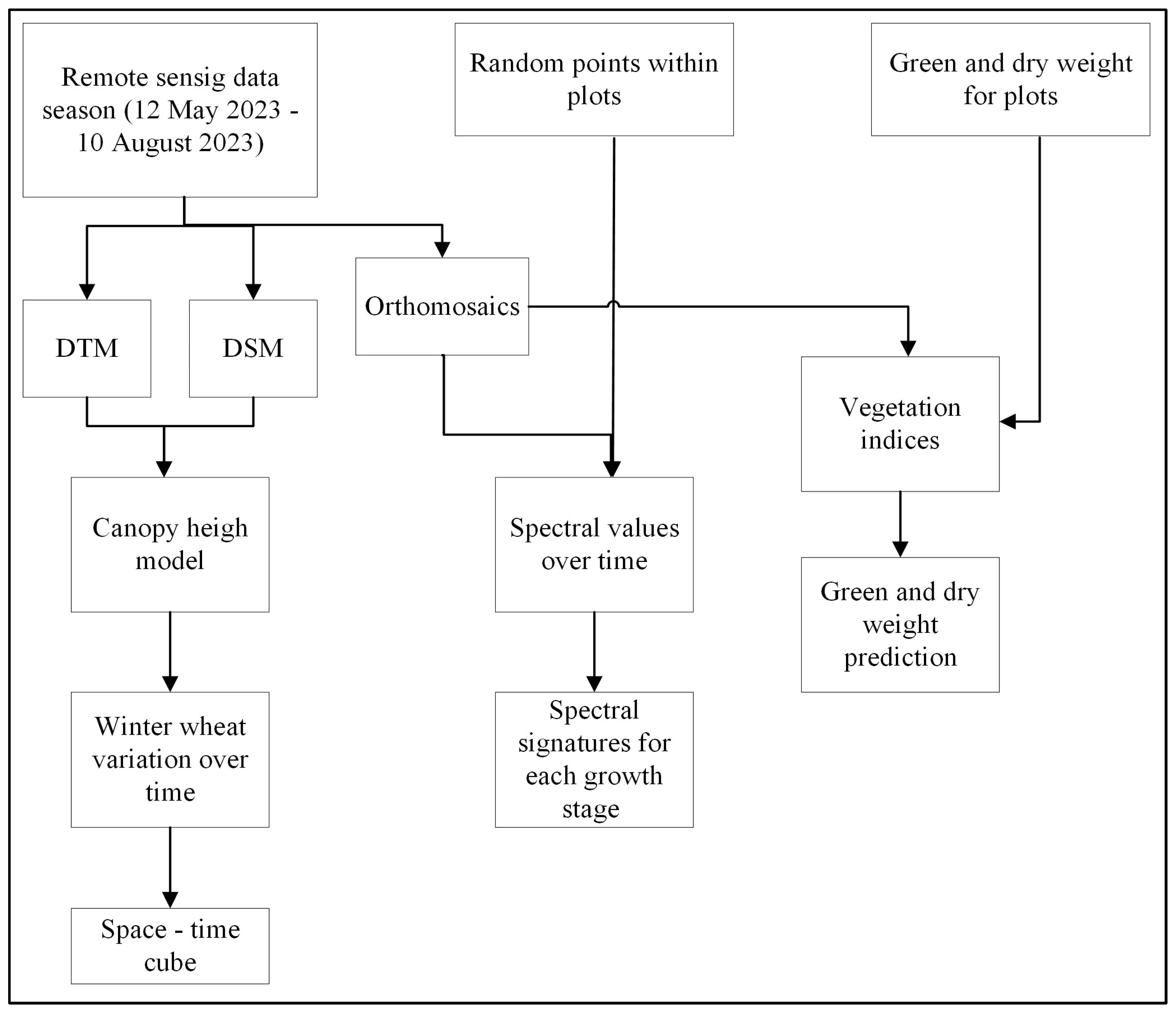
2. Materials and Methods

2.1. Study Area and Data

The research was conducted at the Lakehead Agriculture Research Station (LUARS) in Thunder Bay, Ontario, Canada (48°18′18′′ N, 89°23′17′′ W). LUARS is the regional agriculture research station that mainly focuses on diversifying the agricultural industry in NWO through small plot research and extension.
LUARS is interested in analyzing different growth stages of winter wheat spectrally and advising regional farmers. The total extent of the study area was 1528 m2. There were 60 experimental plots of 4.5 m2 (Figure 1). They were treated with different nitrogen content before seeding. However, this is considered a scoping study, and we will repeat the same study next year to confirm the results.
Remote sensing images were acquired using a Remotely Piloted Aircraft System (RPAS or drone) regularly over the growing season (12 May 2023 to 10 August 2023). The RPAS (DJI M300) was equipped with the Micasense RedEdge Mx multispectral camera (MicaSense, Inc., Seattle, USA) [22], which provides blue, green, red, RedEdge and Near-Infrared (NIR) bands at very high spatial resolution (sensor dimensions = 1280 × 960 px). The details about the central wavelengths and bandwidths of the sensor can be seen in (Table 1).
Images were acquired ten times between 12 May 2023 and 10 August 2023. The imaging period covers various winter wheat growth stages, including the heading, flowering, milk, dough, and ripening stages [6]. Initially, the RPAS was flown at 60 m above ground, but later, it was 30 m above ground to get 4 cm spatial resolution. The images were processed with the specialized software Pix4DMapper (version 4.9) [23] and generated orthomosaics, Digital Elevation Models (DEMs) and Digital Surface Models (DSMs) of the study area (Figure 2).

2.2. Spectral Signatures of Winter Wheat at Different Growing Stages

Random points (2000) were generated within winter wheat plots, and spectral values for each band over time were extracted (Figure 2). Finally, the spectral profiles were generated and analyzed according to different growing stages (Table 2). Additionally, photographs taken in the field were used to compare them with the spectral variability of each stage.

2.3. Analysis of Winter Wheat Height Variation over Time

A Canopy Height Model (CHM) represents the height of winter wheat canopies above ground, and it can be generated using Equation (1):
C H M = D S M D E M
where DSM: Digital Surface Model and DEM: Digital Elevation Model.
CHMs for all imaging dates were created by using Equation (1). Then, the corresponding CHM values for each random point over time were extracted.

Space–Time Cube

A space–time cube is a powerful conceptual and analytical tool used in Geographic Information Systems (GIS) to visualize and analyze spatiotemporal data. By utilizing a space–time cube, spatiotemporal data can be analyzed in the form of time series analysis, the integrated analysis of spatial and temporal patterns, and 2D and 3D visualization techniques. In each location-defined cube container, the count of observations for that container in that time period and any summary field variable or statistic is calculated. The trend of container values over time at each location is measured using the Mann–Kendall statistic [18]. Figure 3 illustrates the structure of a space–time cube for defined locations, which simultaneously represents three dimensions of space (x, y, z) and one dimension of time (t), enabling analysts to explore and understand how phenomena change both in space and time. Within the cube, data attributes are assigned to the spatial and temporal dimensions [18].
The time series of CHM values for random points were binned for a ten-day interval and the STC was created.
The height variation of each plot over time was analyzed. The time series clustering, which identifies the locations in the space–time cube that are most similar, was tested. The temporal series were created based on three criteria: values consistent over time, simultaneous growth trends increasing or decreasing, and similar repetitive patterns. The repeated patterns were detected through functional data analysis using a Fourier family [24]. Also, STC was checked for emerging hot spots to see whether there was a sudden growth of plots within that period.

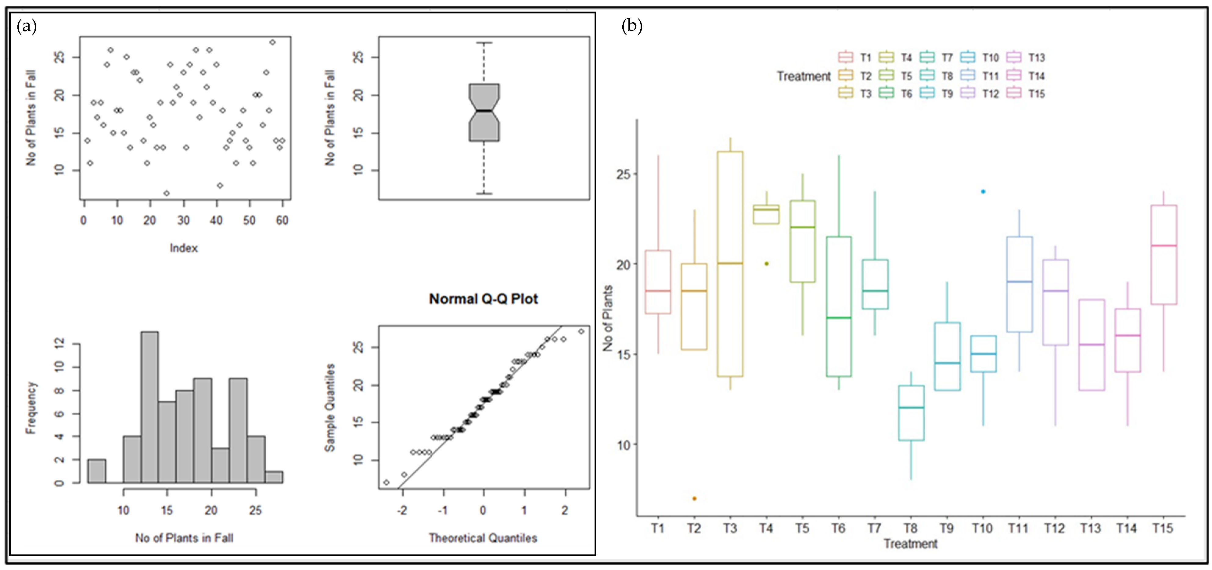
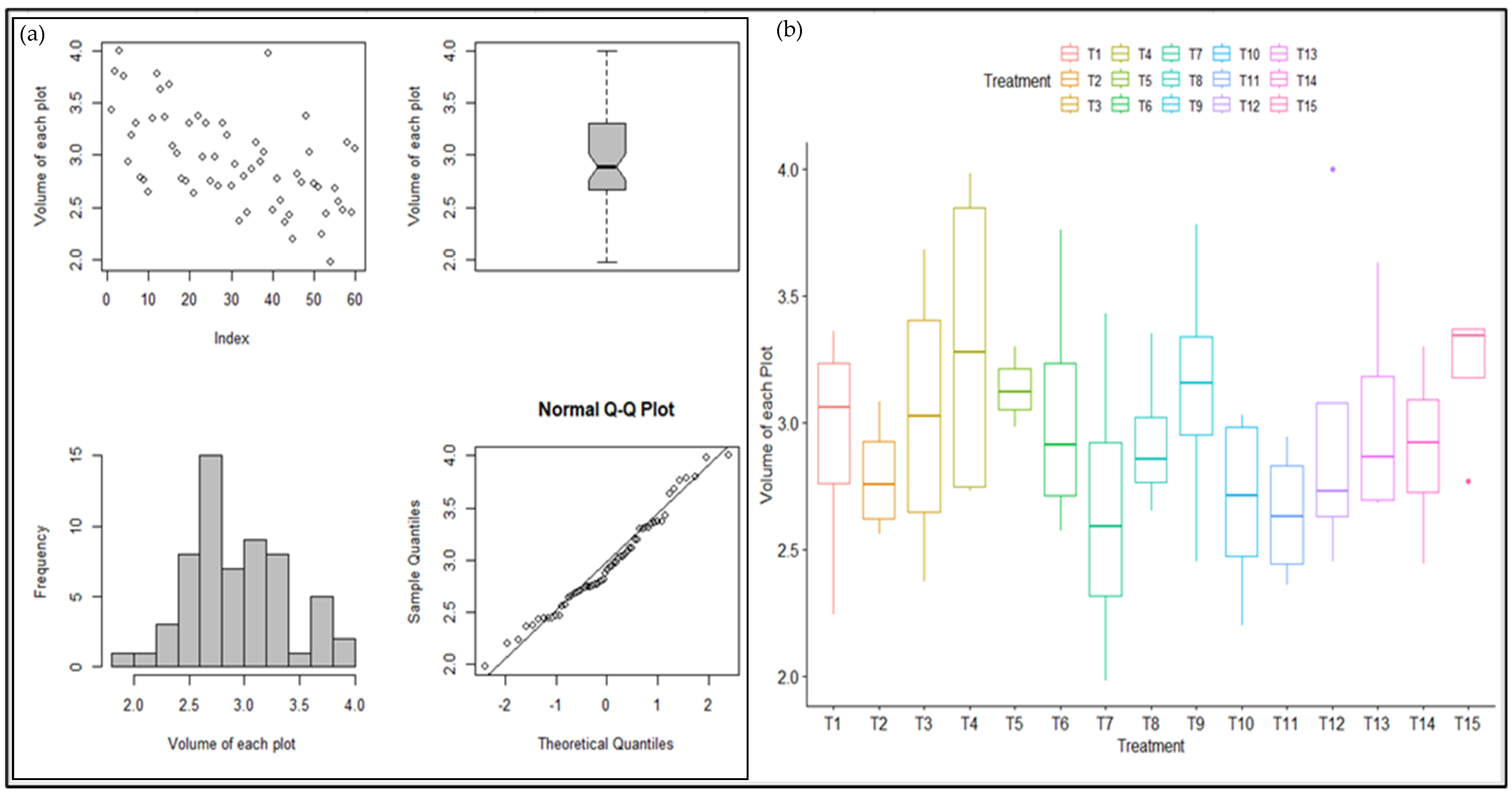
2.4. Statistical Analysis of Winter Wheat Growth Pattern

A statistical analysis of winter wheat’s canopy volume at the ripening stage, the no. of plants that emerged in spring, and the green and dry weights after harvesting was conducted concerning each plot’s nitrogen content. First, the data were cleaned for errors and outliers. At this stage, outliers were noted and deleted manually in MS Excel 2021. Then, an exploratory data analysis (EDA) was conducted using scatter plots, histograms, box plots, and normal Q-Q plots. This was designed for preliminary investigations on data to discover patterns, detect anomalies, test hypotheses, and validate assumptions using summary statistics and graphical representations [25]. Hence, outliers were further detected and removed manually based on box plots. Once the EDA was completed, an appropriate statistical test was selected to examine the homogeneity of variances between treatments and the collected data. Table 3 shows the description of different treatments.

2.5. Estimating Winter Wheat Yield Using Remote Sensing

Machine learning algorithms and remote sensing have opened a new era of precision agriculture, especially in estimating crop yield over linear regression algorithms. Among various algorithms, the XGBoost (Extreme Gradient Boost) machine learning algorithm is well-known for providing better solutions regardless of the data types [26]. This study tested linear regression and the XGBoost algorithm to predict the crop yield using remote sensing.
As shown in Table 4, vegetation indices (VIs) were calculated for images at the end of the flowering stage (12 July 2023), the dough stage (20 July 2023) and the beginning of the ripening stage (29 July 2023). These VIs were selected based on their ability to detect the chlorophyll content, canopy moisture and greenness. It is well-known that the dough stage reflects the yield better in remote sensing images; therefore, this study selected the images before and after the dough stage for analysis.
The average VIs for each field plot were calculated based on “Zonal Statistics”. The correlation between green fresh weight of harvest and the indices were analyzed. The VIs with the highest correlation were tested for linear regression. After that, XGBoost algorithm was used to predict the winter wheat yield for this season. The xgboost package in R software 4.1.2 [34] was used with GCI and DVI for 12 July and 20 July images and RECI, NDVI, and NDRE for 20 July image as predictor variables. Since there were 60 green weight data points (corresponds to 60 plots in the study area), 70% of them were used to train the model and the remaining were used for cross validation. The model was initially trained 100 times as a tree booster with eta = 0.09; gamma = 10; max_depth = 10; and sub_sample = 0.5. After few iterations, the optimal model was created with nine rounds. The cross-validation results found the optimal parameters for the XGBoost model.

3. Results

3.1. Spectral Profiles

Figure 4 shows the spectral signatures for each growth stage. NIR values increased from heading to the flowering stages and slightly decreased at the milk stage. The lowest NIR values were at the ripening stage. Red Edge values were highest at the dough and ripening stages. The lowest green values were at the flowering stage.

3.2. Analysis of Witner Wheat Hight Variation over Time

The STC allowed the observation of the canopy height variation over time. Figure 5 shows the average height variation. The height values were reduced from 16 May 2023 to mid-June and then gradually increased till early August. There were some errors with the data acquired on 8 June 2023 and it was reflected in the graph as a negative value in mid-June. Winter wheat had already been harvested by the last day of photography.

3.2.1. Times Series Clustering

Field plots were grouped into categories with similar heights over time using time series clustering tool (Figure 6). They were separated into five categories (similar in height variation over time). Figure 6 shows a direct comparison of winter wheat plots based on their nitrogen content (T1 to T15) and height variations. It is observed that the different treatments applied to the plots did not directly influence the variation in the height of winter wheat over time. For example, the plots with “T4” treatment clustered with three and five plots and found an isolated one as well. The heights of plots with no nitrogen treatments (112, 208, 304, 411) were similar to two or three neighboring plots, which had different treatments (Figure 6).

3.2.2. Local Outlier Analysis

Local cluster–outlier analysis was done to identify significant clusters and outliers in terms of canopy height over time. However, these plots had no significant high–high or high–low clusters; instead, multiple types of statically significant clusters were identified over time. For instance, once, a plot was a low–high outlier, and in another period, it was a part of the high–high cluster. There were no uniform clustering patterns during the period. When considering the entire cube, there were six high–low outliers, 60 low–low cluster and 253 not significant cubes. The highest number of high–low outliers were from 1–11 June 2023, mainly due to the inaccurate CHM value on the 8 June 2023 dataset.

3.3. Statistical Analysis of Winter Wheat Growth Pattern

Four types of graphs were examined to check the presence of outliers and the data normality. The statistical analysis results determined the data normality for several variables. From Figure 7, Figure 8, Figure 9, Figure 10 and Figure 11, the scatter plot shows the degree of scatter of variables concerning the order of data entry. The horizontal axis “Index” represents the order in which the points appear in the data file. For example, in Figure 7a, data points are not trended or patterned with the order of the entry, and the degree of scatter is consistent. According to the box plot, there were no outliers in the plant count in autumn. The Shapiro–Wilk normality test results were not statistically significant. Hence, data were normally distributed. This was also evident in the Normal Q–Q plot. An ANOVA test was conducted to evaluate the homogeneity of variance between the plant count in autumn and the treatments applied. The result showed that the variance is not statistically significant, implying no difference between the number of plants in autumn and the different treatments applied (Figure 7b). When looking at individual treatments, there were outliers for T2, T4 and T10. Other data were normally distributed without (Figure 7a).
The Flinger test was applied to determine the homogeneity of variance between plant counts in spring and the treatments applied to each plot. The results showed that the variance is not statistically significant, suggesting no difference between the number of plants in spring and the different treatments applied.
Figure 9 shows the EDA of canopy volume (m3) at the dough stage, assuming that they were almost ready to harvest. Data were normally distributed (Figure 9a) and ANOVA results were not statistically significant (Figure 9b), indicating no difference between the volume of plants per plot and the different treatments applied.
The EDA results for each plot’s green fresh weight (g/plot) and dry weight (g/plot) did not show any outliers, and the data were normally distributed (Figure 10 and Figure 11). When the ANOVA test was performed on green weight, the results revealed that the homogeneity of variance between green weight data and treatments in each plot presented a significant difference (Figure 10b). This was confirmed by conducting the Tukey test, which determined that the difference was only between treatments T8/T4 and T8/T10, as seen in the graph in (Figure 10b). For the dry weight analysis, the ANOVA results presented significant differences and then (Figure 11b) the Tukey test was applied, and, as seen in (Figure 11b), it was determined that there was a difference between treatments T8/T4 and T8/T10.

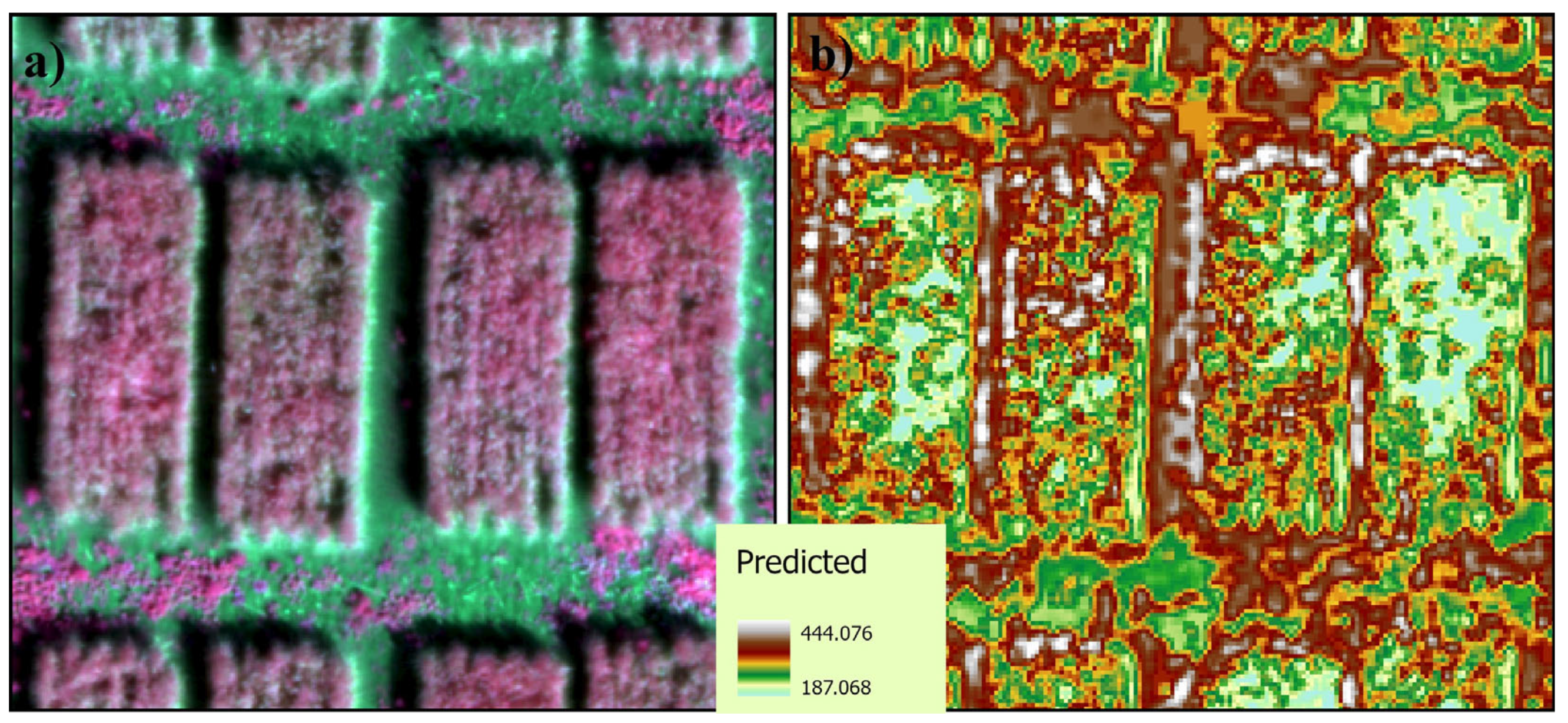
3.4. Yield Estimation

The correlation between green weight and vegetation indices was considered to select the most suitable indices for further calculations. All indices with a correlation greater than 0.4 were selected for three dates (Table 5). However, the linear regression model between those VIs and green weight was not statistically significant, and none of the model parameters were also statistically significant, contributing to explaining the yield in each plot.
The XGBoost model was iterated to obtain the optimal model parameters. The parameter gamma controls the overfitting, and the optimal value found for this study was four; max_depth controls the depth of the booster tree, and the optimal value was six. The ideal number of rounds was nine. Default values were used for the remaining parameters.
The XGBoost model received moderate results. The R-square values between predicted and validation green weight samples were 0.5, and the Root Mean Square Error (RMSE) was 70 g for all plots, which means 1.67 g per plot of 4.5 m2. The spatial distribution of the winter wheat yield map captured the spatial variation within plots, although there were some underestimations. For example, Figure 12a shows how the remote sensing image varied the spectral reflectance in the dough stage, and Figure 12b shows how the variation was captured by the XGBoost algorithm. The areas with higher NIR values showed low yield prediction. This is obvious from the spectral signature of crops; at the ripening stage, NIR values are lower, and green reflectance is high.

4. Discussion

The study used remote sensing techniques to evaluate 60 experimental winter wheat plots for their growth dynamics. Remotely sensed data were acquired from Micasense RedEdge MX camera with five spectral bands over five growing stages.

4.1. Spectral Profiles

The spectral profiles in different growth phases aligned with previous research, emphasizing the importance of Near-Infrared (NIR) reflectance in assessing vegetation health [35]. As winter wheat progressed through its growth stages (heading to flowering), an increase in NIR reflectance was observed, indicative of an increase in biomass and vegetation cover. According to Peng et al. [35], this reaffirms the relationship between NIR reflectance and healthy vegetation, attributed to the biomass and vegetation cover of thriving plants. This is the plant’s green-up, stem elongation, and green heading period. However, a decrease in NIR was exhibited from the milk stage to the ripening stage. The milk stage begins after the head completely emerges, and flowering starts from the middle and continues to the top in yellow color [6]. Hence, NIR reflectance was reduced, while green and red (which creates yellow) reflectance were slightly increased. The color changes were also evident in the photographs related to each stage (Figure 4).
The analysis of the red band revealed an increase in reflectance as the wheat transitioned from the flowering phase to maturity, which, according to Xie et al. [36], indicates the transition from high photosynthetic activity to full maturity. For instance, the plant is brownish at the ripening stage with no or minimum photosynthesis activities, so the red band reflected more. This increase in red band reflectance suggests changes in chlorophyll and leaf structure. As for the RedEdge band, a consistent increase in reflectance was observed as the wheat transitioned from the flowering phase to maturity, which may indicate vegetation maturation and the transition from high photosynthetic activity to full maturity [37].

4.2. Analysis of Winter Wheat Height Variation over Time

The observed sudden height decrease in Figure 5 from May to June 13 was attributed to the potential errors in image capturing on 8 June 2023. There were some issues with Ground Control Points (GCPs) and, thus, canopy heights. As Tong Qingxi et al. [38] suggested in their study, the STC provided helpful insight for monitoring and characterizing winter wheat over time. For example, after 13 June 2023, the average winter wheat height gradually increased until late July, which is the ripening period, as an indicator of successful growth.
The “Time Series Clustering” analysis partitions a collection of height values over time into categories based on their similarities in height changes. Mostly, the neighboring plots created clusters (similar in height) regardless of their nitrogen treatments. However, some isolated plots (206, 210, 212) had relatively high nitrogen input, and their average individual heights were higher than the surrounding plots. To the authors’ knowledge, no study has tested winter wheat height variation over time using STC; however, Marino et al. [36] tested the application of STC for the VI value variation over time for winter wheat. They indicated STC’s effectiveness for monitoring winter wheat and assessing vegetation traits.
The “Local Outlier Analysis” using STC highlights the height clusters and outliers in space and time. No significant clusters were noted; instead, the height of plots alternated from low–high clusters to high–high clusters, etc., over time due to various conditions. Since the agriculture in NWO is rainfed, plants can grow fast during the rainy period, satisfying the optimal growing conditions for winter wheat growing. Therefore, this tool is useful for anomaly detection within plots and, thus, an excellent alternative for smart agriculture practices. Moso et al. [39] emphasized how anomaly detection could improve harvesting efficiency and crop health.
Although this study did not carry out an in-depth analysis of winter wheat height versus different treatments, the usefulness of STC in the context of smart agriculture is clear. In future studies, we suggest creating space–time cubes for individual plots to analyze in situ height variations.

4.3. Statistical Analysis of Winter Wheat Growth Pattern

The statistical analysis of different factors revealed interesting insights into the effects of nitrogen treatments in various quantities. Despite applying different nitrogen quantities, no significant differences were observed in plant count during autumn and spring, nor in wheat height and volume across different plots at maturity. This finding suggests a consistent response of winter wheat to nitrogen treatments, indicating a level of uniformity in its growth behavior. Although there were no statistically significant differences between various treatments and volumes, the green and dry weight was statistically significant in several plots. It is worth noting that these results align with previous studies, such as that of Yue et al. [40], which emphasize the importance of nitrogen application in influencing winter wheat yield and crop weight variation. Specifically, treatments T8/T4 and T8/T10 exhibited notable discrepancies, with T8 showing the lowest values and T4 and T10 showing the highest weights. These observations demonstrate an interaction between nitrogen application and biomass production. Treatment T8 may have had a detrimental effect on biomass production, while T4 and T10 appear to have had a positive influence, as evidenced by the weights obtained. This highlights the importance of nitrogen in the growth dynamics of winter wheat despite the absence of significant effects on other parameters [40]. However, the authors do not draw any conclusions as the study did not consider the other influencing factors, such as a complete profile of soil nutrients and moisture and weather.

4.4. Estimating Winter Wheat Yield

All possible combinations of the linear regression of green weight and predictors did not show statistically significant results. Hence, linear regression modelling is not an option for predicting winter wheat yield in this study. This might result in differences in green weights corresponding to different treatments (Figure 9b). The other main concern is that the study considered the average green weight and the VI values per plot. The green weight and spectral values might vary spatially depending on the soil nutrient profile. Hence, using sub-sampling plots (several sub plots within each plot) and analyzing the spectral variations accordingly is recommended. The result obtained from the XGBoost model yielded an R-square value of 0.5 and a Root Mean Squared Error (RMSE) of 1.67 g per plot, indicating a reasonable level of predictive capability. The performance of the XGBoost model in estimating winter wheat yield, as evidenced in this study, suggests a moderate level of predictive ability, albeit with some discrepancies between predicted and actual values. Rohit et al. [41] also employed the XGBoost algorithm for yield estimation and highlighted the high accuracy in yield prediction. However, these studies cannot be directly compared due to different environmental conditions. It is important to note that discrepancies in model performance may stem from various factors, such as the unique characteristics of the dataset and crop species considered, as well as the environmental variables incorporated in each research framework.

5. Conclusions

The study analyzed the growth dynamics of winter wheat using high spatial and temporal resolution optical images. The images were acquired from the Remotely Piloted Aircraft System over the growth season, and field samples were collected. First, the spectral signature of winter wheat for five growing stages (heading, flowering, milk, dough and ripening) was created using spectral reflectance values for random points (2000) for each growth stage. These profiles confirmed an increase in NIR reflectance with the crop’s maturing phase, associated with an increase in biomass and vegetative cover and a decrease as it reached senescence. Results were in agreement with the existing literature linking NIR reflectance with the growth and health of vegetation. Then, a space–time cube (STC) was created for average canopy heights over time. A measure of the change in winter wheat height over time was carried out. Variations in winter wheat height at different stages were identified, and it was determined that the use of different treatments could be associated with these differences. However, it was not possible to ascertain which treatment would be ideal for winter wheat growth due to the multiple plots treated similarly being segregated into diverse growth categories as determined by the Time Series Clustering tool. A decrease between 30 May and 13 June was observed due to possible image acquisition errors. The statistical analysis of the number of winter wheat plants in autumn and spring or volume and height at maturity revealed no statistically significant differences with various nitrogen treatments. However, notable differences were discernible in both green and dry weights. This suggests that nitrogen treatment did have an effect on biomass production in winter wheat. Finally, winter wheat yield was estimated using XGBoost machine learning algorithms with moderate results. Vegetation Indices (ten) were derived from images acquired over three days during the dough and ripening stages. The most suitable indices were used for the final modelling (correlation greater than 0.4 with the green weight of winter wheat). The accuracy of the spatial distribution of the green weight map was 0.5, and the Root Mean Square Error was 1.67 g per plot. The study recommended creating space–time cubes for individual plots and testing XGBoost algorithms more rigorously to train samples for yield prediction. However, in conclusion, this study demonstrated the usefulness of incorporating high spatial and temporal resolution optical images and various analysis tools for monitoring the growth dynamics of winter wheat.

Author Contributions

Conceptualization: M.V.B.F., M.K.H., T.S.S. and L.S.S.; methodology: M.V.B.F. and M.K.H.; field set up and data collection: T.S.S. and M.K.H.; analysis and validation: M.V.B.F., M.K.H. and L.S.S.; writing—original draft preparation: M.V.B.F.; writing—review and editing: M.K.H., L.S.S. and T.S.S.; project administration: T.S.S., M.K.H. and M.V.B.F.; funding acquisition: M.K.H. and T.S.S. All authors have read and agreed to the published version of the manuscript.

Funding

This research was funded by the Agri Risk Initiative Program, Agriculture and Agri-Food Canada, Microgrant number: ARI-IAR-MG-23.

Data Availability Statement

The data is available and can be obtained by directly contacting the author.

Acknowledgments

We express our sincere gratitude to Reg Nelson, Samiul Alam and Gurleen Kaur for their assistance in data collection, and the technical staff at Lakehead University Agriculture Research Station for their support. Additionally, we thank colleagues who, in various ways, provided guidance and information during this research.

Conflicts of Interest

The authors declare no conflicts of interest.

References

  1. Ruane, A.C.; Rosenzweig, C. Climate Change Impacts on Agriculture. In Agriculture & Food Systems to 2050; World Scientific: Singapore, 2018; pp. 161–191. [Google Scholar] [CrossRef]
  2. Feng, X.; Tian, H.; Cong, J.; Zhao, C. A method review of the climate change impact on crop yield. Front. For. Glob. Chang. 2023, 6, 1198186. [Google Scholar] [CrossRef]
  3. Government of Canada. Climate Change Impacts on Agriculture. 2020. Available online: https://agriculture.canada.ca/en/environment/climate-change/climate-scenarios-agriculture (accessed on 28 October 2023).
  4. Government of Canada. The Biology of Triticum aestivum L. (Wheat). 2014. Available online: https://inspection.canada.ca/plant-varieties/plants-with-novel-traits/applicants/directive-94-08/biology-documents/triticum-aestivum-l-/eng/1330982915526/1330982992440 (accessed on 24 August 2023).
  5. Zong, J.; Ontario Is an Agricultural Powerhouse That Leads in Many Farming Categories. Canadian Agriculture at a Glance. Available online: https://www150.statcan.gc.ca/n1/pub/96-325-x/2021001/article/00006-eng.htm (accessed on 28 October 2023).
  6. Ontario Ministry of Agriculture Food and Rural Affairs. A Visual Guide to Winter Wheat Staging. Grain Farmers of Ontario. 2023. Available online: https://gfo.ca/wp-content/uploads/2023/02/Grain-Farmers-of-Ontario-Cereal-Staging-Guide-223on_compressed.pdf (accessed on 5 February 2024).
  7. Singh, P.; Pandey, P.C.; Petropoulos, G.P.; Pavlides, A.; Srivastava, P.K.; Koutsias, N.; Deng, K.A.K.; Bao, Y. Hyperspectral remote sensing in precision agriculture: Present status, challenges, and future trends. In Hyperspectral Remote Sensing; Elsevier: Amsterdam, The Netherlands, 2020; pp. 121–146. [Google Scholar]
  8. Xie, Y.; Wang, C.; Yang, W.; Feng, M.; Qiao, X.; Song, J. Canopy hyperspectral characteristics and yield estimation of winter wheat (Triticum aestivum) under low temperature injury. Sci. Rep. 2020, 10, 244. [Google Scholar] [CrossRef] [PubMed]
  9. Morales, G.; Sheppard, J.; Logan, R.; Shaw, J. Hyperspectral Band Selection for Multispectral Image Classification with Convolutional Networks. In Proceedings of the 2021 International Joint Conference on Neural Networks (IJCNN), Shenzhen, China, 18–22 July 2021; pp. 1–8. [Google Scholar] [CrossRef]
  10. Guarnera, C.; Multispectral Imaging in Precision Agriculture: An In-Depth Guide. Blue Falcon Aerial. Available online: https://www.bluefalconaerial.com/how-multispectral-drones-work/ (accessed on 28 October 2023).
  11. Ma, C.; Liu, M.; Ding, F.; Li, C.; Cui, Y.; Chen, W.; Wang, Y. Wheat growth monitoring and yield estimation based on remote sensing data assimilation into the SAFY crop growth model. Sci. Rep. 2022, 12, 5473. [Google Scholar] [CrossRef] [PubMed]
  12. Liu, S.; Peng, D.; Zhang, B.; Chen, Z.; Yu, L.; Chen, J.; Pan, Y.; Zheng, S.; Hu, J.; Lou, Z.; et al. The Accuracy of Winter Wheat Identification at Different Growth Stages Using Remote Sensing. Remote Sens. 2022, 14, 893. [Google Scholar] [CrossRef]
  13. Han, X.; Wei, Z.; Chen, H.; Zhang, B.; Li, Y.; Du, T. Inversion of Winter Wheat Growth Parameters and Yield Under Different Water Treatments Based on UAV Multispectral Remote Sensing. Front. Plant Sci. 2021, 12, 609876. [Google Scholar] [CrossRef] [PubMed]
  14. Cintas, J.; Franch, B.; Van-Tricht, K.; Boogaard, H.; Degerickx, J.; Becker-Reshef, I.; Moletto-Lobos, I.; Mollà-Bononad, B.; Sobrino, J.A.; Gilliams, S.; et al. TRANCO: Thermo radiometric normalization of crop observations. Int. J. Appl. Earth Obs. Geoinf. 2023, 118, 103283. [Google Scholar] [CrossRef]
  15. Zhang, X.-W.; Liu, J.-F.; Qin, Z.; Qin, F. Winter wheat identification by integrating spectral and temporal information derived from multi-resolution remote sensing data. J. Integr. Agric. 2019, 18, 2628–2643. [Google Scholar] [CrossRef]
  16. Cheng, E.; Zhang, B.; Peng, D.; Zhong, L.; Yu, L.; Liu, Y.; Xiao, C.; Li, C.; Li, X.; Chen, Y.; et al. Wheat yield estimation using remote sensing data based on machine learning approaches. Front. Plant Sci. 2022, 13, 1090970. [Google Scholar] [CrossRef] [PubMed]
  17. Badea, A.; Badea, G. An Overview on Space Time Cube Visualization in Gis; Researchgate: Berlin, Germany, 2018. [Google Scholar]
  18. ESRI. How Create Space Time Cube Works. 2023. Available online: https://pro.arcgis.com/en/pro-app/latest/tool-reference/space-time-pattern-mining/learnmorecreatecube.htm?ssp=1&darkschemeovr=1&setlang=en-CA&safesearch=moderate (accessed on 28 November 2023).
  19. Krishnan, P.; Aggarwal, P.; Mridha, N.; Bajpai, V. Spatio-Temporal Changes in Wheat Crop Cultivation in India. ISPRS—Int. Arch. Photogramm. Remote Sens. Spat. Inf. Sci. 2019, XLII-3/W6, 385–395. [Google Scholar] [CrossRef]
  20. El Imanni, H.S.; El Harti, A.; El Iysaouy, L. Wheat Yield Estimation Using Remote Sensing Indices Derived from Sentinel-2 Time Series and Google Earth Engine in a Highly Fragmented and Heterogeneous Agricultural Region. Agronomy 2022, 12, 2853. [Google Scholar] [CrossRef]
  21. Liu, Y.; Sun, L.; Liu, B.; Wu, Y.; Ma, J.; Zhang, W.; Wang, B.; Chen, Z. Estimation of Winter Wheat Yield Using Multiple Temporal Vegetation Indices Derived from UAV-Based Multispectral and Hyperspectral Imagery. Remote Sens. 2023, 15, 4800. [Google Scholar] [CrossRef]
  22. MicaSense. Comparison of MicaSense Cameras, Seattle, USA. Available online: https://support.micasense.com/hc/en-us/articles/1500007828482-Comparison-of-MicaSense-Cameras (accessed on 22 November 2023).
  23. PIX4D. PIX4Dmapper version 4.9. Available online: https://www.pix4d.com/product/pix4dmapper-photogrammetry-software/ (accessed on 10 December 2023).
  24. ESRI. Time Series Clustering (Space Time Pattern Mining). ArcGIS Pro. Available online: https://pro.arcgis.com/en/pro-app/3.1/tool-reference/space-time-pattern-mining/time-series-clustering.htm#:~:text=Time%20series%20can%20be%20clustered,by%20cluster%20membership%20and%20messages (accessed on 9 December 2023).
  25. Patil, P. What is Exploratory Data Analysis? Towards Data Science. 2018. Available online: https://towardsdatascience.com/exploratory-data-analysis-8fc1cb20fd15 (accessed on 26 November 2023).
  26. Moslemi, A. A tutorial-based survey on feature selection: Recent advancements on feature selection. Eng. Appl. Artif. Intell. 2023, 126, 107136. [Google Scholar] [CrossRef]
  27. Kawashima, S.; Nakatani, M. An Algorithm for Estimating Chlorophyll Content in Leaves Using a Video Camera. Ann. Bot. 1998, 81, 49–54. [Google Scholar] [CrossRef]
  28. Daughtry, C.S.T.; Walthall, C.L.; Kim, M.S.; De Colstoun, E.B.; McMurtrey, J.E., III. Estimating Corn Leaf Chlorophyll Concentration from Leaf and Canopy Reflectance. Remote Sens. Environ. 2000, 74, 229–239. [Google Scholar] [CrossRef]
  29. Gitelson, A.A.; Viña, A.; Ciganda, V.; Rundquist, D.C.; Arkebauer, T.J. Remote estimation of canopy chlorophyll content in crops. Geophys. Res. Lett. 2005, 32, L08403. [Google Scholar] [CrossRef]
  30. Rouse, J.W.; Haas, R.H.; Schell, J.A.; Deering, D.W. Monitoring vegetation systems in the Great Plains with ERTS. In Third Earth Resources Technology Satellite-1 Symposium-Volume I: Technical Presentations; NASA: Washington, DC, USA, 1974. [Google Scholar]
  31. Gitelson, A.A.; Gritz, Y.; Merzlyak, M.N. Relationships between leaf chlorophyll content and spectral reflectance and algorithms for non-destructive chlorophyll assessment in higher plant leaves. J. Plant Physiol. 2003, 160, 271–282. [Google Scholar] [CrossRef] [PubMed]
  32. Gitelson, A.A.; Merzlyak, M.N. Remote estimation of chlorophyll content in higher plant leaves. Int. J. Remote Sens. 1997, 18, 2691–2697. [Google Scholar] [CrossRef]
  33. Jiang, Z.; Huete, A.R.; Didan, K.; Miura, T. Development of a two-band enhanced vegetation index without a blue band. Remote Sens. Environ. 2008, 112, 3833–3845. [Google Scholar] [CrossRef]
  34. Chen, T.; Guestrin, C. XGBoost: A Scalable Tree Boosting System. In Proceedings of the KDD ’16: 22nd ACM SIGKDD International Conference on Knowledge Discovery and Data Mining, San Francisco, CA, USA, 13–17 August 2016; Association for Computing Machinery: New York, NY, USA, 2016; pp. 785–794. [Google Scholar] [CrossRef]
  35. Peng, Y.; Zhang, M.; Xu, Z.; Yang, T.; Su, Y.; Zhou, T.; Wang, H.; Wang, Y.; Lin, Y. Estimation of leaf nutrition status in degraded vegetation based on field survey and hyperspectral data. Sci. Rep. 2020, 10, 4361. [Google Scholar] [CrossRef] [PubMed]
  36. Marino, S.; Alvino, A. Vegetation Indices Data Clustering for Dynamic Monitoring and Classification of Wheat Yield Crop Traits. Remote Sens. 2021, 13, 541. [Google Scholar] [CrossRef]
  37. Xie, Q.; Dash, J.; Huang, W.; Peng, D.; Qin, Q.; Mortimer, H.; Casa, R.; Pignatti, S.; Laneve, G.; Pascucci, S.; et al. Vegetation Indices Combining the Red and Red-Edge Spectral Information for Leaf Area Index Retrieval. IEEE J. Sel. Top. Appl. Earth Obs. Remote Sens. 2018, 11, 1482–1493. [Google Scholar] [CrossRef]
  38. Qingxi, T.; Xia, Z.; Bing, Z.; Jihua, W. Crop growth monitoring study by using multi-temporal index image cube analysis. In Proceedings of the IEEE 2002 International Conference on Communications, Circuits and Systems and West Sino Expositions, Chengdu, China, 29 June–1 July 2002; pp. 1596–1601. [Google Scholar]
  39. Moso, J.C.; Cormier, S.; de Runz, C.; Fouchal, H.; Wandeto, J.M. Anomaly Detection on Data Streams for Smart Agriculture. Agriculture 2021, 11, 1083. [Google Scholar] [CrossRef]
  40. Yue, S.; Meng, Q.; Zhao, R.; Ye, Y.; Zhang, F.; Cui, Z.; Chen, X. Change in Nitrogen Requirement with Increasing Grain Yield for Winter Wheat. Agron. J. 2012, 104, 1687–1693. [Google Scholar] [CrossRef]
  41. Rohit, R.; Baranidharan, B. Crop Yield Prediction using XG Boost Algorithm. Int. J. Recent Technol. Eng. 2020, 5, 2277–3878. Available online: https://www.researchgate.net/publication/364028532_Crop_Yield_Prediction_using_XG_Boost_Algorithm (accessed on 2 February 2024).
Figure 1. The study area map (part of Lakehead University Agricultural Research Station). The winter wheat plots are represented with red polygons and are numbered according to different nitrogen treatments.
Crops 04 00009 g001
Figure 2. The overall workflow of the project.
Crops 04 00009 g002
Figure 3. The structure of the space–time cube for defined locations (adapted from https://www.esri.com, accessed on 29 November 2023).
Crops 04 00009 g003
Figure 4. Spectral signatures of winter wheat at different growth stages. Spectral profiles (left) and corresponding field photo (right) for each stage.
Crops 04 00009 g004
Figure 5. Average canopy height over time for ten days intervals, extracted from the space–time cube.
Crops 04 00009 g005
Figure 6. Results of Times Series Clustering Analysis.
Crops 04 00009 g006
Figure 7. (a) Exploratory Data Analysis (EDA) of number of plants in autumn; (b) No. of plants with respect to each treatment in autumn.
Crops 04 00009 g007
Figure 8. (a) Exploratory Data Analysis (EDA) of the number of plants in spring; and (b) No. of plants with respect to each treatment in spring.
Crops 04 00009 g008
Figure 9. (a) Exploratory Data Analysis (EDA) for the volume (m3) obtained per plot; and (b) Volume of each plot based on different treatments.
Crops 04 00009 g009
Figure 10. (a) Exploratory Data Analysis (EDA) for green weight (g/plot) data; and (b) Green weight (g/plot) based on different treatments.
Crops 04 00009 g010
Figure 11. (a) Exploratory Data Analysis (EDA) for dry weight (g/plot) data; and (b) Dry weight (g/plot) based on different treatments.
Crops 04 00009 g011
Figure 12. (a) A remote sensing image acquired on 20 July 2023, in standard false colors and (b) the spatial distribution of winter wheat yield prediction.
Crops 04 00009 g012
Table 1. Central wavelength and bandwidth data for each sensor (Adapted from: https://support.micasense.com/hc/en-us/articles/360011389334-RedEdge-MX-Integration-Guide, accessed on 23 November 2023).
Band NameCenter Wavelength (NM)Bandwidth (NM)
Blue47532
Green 56027
Red66814
Red Edge71712
NIR84257
Table 2. Different growing stages correspond to a visual guide to winter wheat staging in Ontario [6] and the corresponding images.
StagesImage Date
Heading12 and 26 May 2023
Flowering8, 16, 23 June 2023
Milk4 and 12 July 2023
Dough20 July 2023
Ripening29 July and 10 August 2023
Table 3. The description of different treatments for each plot and the components. The location of each plot is available in Figure 1.
TreatmentsNitrogen ContentPlots
T1No nitrogen411, 208, 112, 304
T230 kg/ha at seeding and 90 kg/ha in early spring410, 105, 210, 312
T3120 kg/ha412,314, 209, 108
T4120 kg/ha (Entec Soil Nitrogen)211, 408, 115, 306
T5120 kg/ha (Urea SuperU)409, 202, 113, 310
T6100 kg/ha (Urea SuperU)214, 414, 101, 308
T790 kg/ha (Urea) and 30 kg/ha (Entec Soil Nitrogen)212, 414, 101, 308
T890 kg/ha (Urea) and 60 kg/ha (Entec Soil Nitrogen)415, 204, 114, 311
T990 kg/ha (Urea) and 90 kg/ha (Entec Soil Nitrogen)206, 405, 313, 103
T1090 kg/ha (Urea) and 30 kg/ha (SuperU)203, 401, 315, 106
T1160 kg/ha (Urea) and 60 kg/ha (SuperU)215, 413, 104, 307
T1230 kg/ha (Urea) and 90 kg/ha (SuperU)213, 407, 102, 305
T1340 kg/ha, 40 kg/ha (Entec Soil Nitrogen) and 40 kg/ha (SuperU)207, 403, 111, 301
T14160 kg/ha (Urea)416, 215, 303, 109
T15120 kg/ha (treated with nitrogen stabilizer)201, 404, 107, 309
Table 4. Different vegetation indices calculated for three images (12,20 and 29 July 2023).
Vegetation IndexEquationReference
Difference Vegetation IndexDVI = G − B[27]
Modified Chlorophyll Absorption in Reflectance IndexMCARI = [(RE − R) − 0.2 × (RE − G)] × (RE/R)[28]
Green Chlorophyll IndexGCI = (NIR/G) − 1[29]
Rededge Chlorophyll IndexRECI = (NIR/RE) − 1[29]
Normalized Difference Vegetation IndexNDVI = (NIR − R)/(NIR + R)[30]
Green Normalized Difference Vegetation IndexGNDVI = (NIR − G)/(NIR + G)[31]
Rededge Normalized Difference Vegetation IndexNDRE = (NIR − RE)/(NIR + RE)[32]
Two-band Enhanced Vegetation IndexEVI2 = 2.5 × [(NIR − R)/(NIR + 2.4 × R + 1)][33]
Note: B = blue; G = green band, R = Red, RE = RedEdge, and NIR = Near-Infrared bands.
Table 5. The selected vegetation indices for green weight prediction in three days.
12 July 202320 July 202329 July 2023
GCI, DVIGCI, RECI, NDVI, NDRE, DVIMCARI, GNDVI, NDRE
Disclaimer/Publisher’s Note: The statements, opinions and data contained in all publications are solely those of the individual author(s) and contributor(s) and not of MDPI and/or the editor(s). MDPI and/or the editor(s) disclaim responsibility for any injury to people or property resulting from any ideas, methods, instructions or products referred to in the content.

