The “Growth Curve”: An Autocorrelation Effect

Abstract

A purposely naïve and semi-empirical model allows for the reproduction of the phenomenological behavior of any real microbial culture by adjusting the values of three parameters, which have a biological meaning only for a virtual microbial culture that mimics the behavior of the real ones. Any genomic, biochemical, and physical peculiarity (microbial species, physiological condition, pH, water activity, temperature, etc.) that distinguishes one real culture from another is “translated” to an effect of the degree of progress of the population density and cell age in the virtual culture. The model leads to a self-consistent description of the growth curve, which looks like the result of an autocorrelation effect. This explains why, in spite of genomic and physiologic differences, all the growth curves show a sigmoid trend. The traditional growth curve and the subsequent exponential decay in the log(N)-vs-t plot can be replaced by straight-line trends when referring to the degree of progress of the population density of the virtual culture.

1. Introduction

Microbial growth is the subject of a vast amount of literature, where the increase by some orders of magnitude of the microbial population density, N, has been reported in a log scale. This is why the so-called “growth curve” [1] is the log(N)-vs-t trend (regardless of the log base), where t stands for the elapsed time. The slope of such a trend, dlog(N)/dt = $k({\displaystyle \frac{\dot{N}}{N}})$—with the Newton notation for the time derivative, where k = 1, log_e(2) and log₁₀(2), for log_e, log₂, and log₁₀ scale, respectively—also corresponds to the expression of the average of $\dot{N}$ over the whole population, N. This is why $({\displaystyle \frac{\dot{N}}{N}})$ is commonly dubbed the “specific growth rate” [2] and referred to as a peculiar property of the “average” single cell that would reflect the underlying biochemical activity during the growth process. A number of authors [3,4,5,6] have since aimed to single out the effects of pH, temperature, ionic strength, specific ionic species, presence of different microbial species, etc., on $({\displaystyle \frac{\dot{N}}{N}})$ and its maximum.

The related formal models tried to assess a connection between the growth curve and some expected processes at the cell level, suggesting adjustable parameters or an alternative presentation of the experimental evidence [7]. The modifications of the early models (logistic, kinetic, Gompertz, Baranyi, etc. [2]), introduced to overcome the mismatch observed in some cases or to improve the best fit of the experimental data, often imply the addition of new parameters, which would correspond to extra processes still at the cell level, like the “physiological state” or pre-inoculation history, etc. [5]. As a result, the biological meaning of such parameters loses reliability, with an improvement in the fit that also is a consequence of their increased number [5,8,9,10,11].

By and large, such a line of interpretation can be rather misleading, as the growth curve indeed concerns the whole system, namely cells + medium, and therefore reflects changes in both them and their correlations with one another [12,13,14,15]. The connection between the observed growth curve and the huge number of underlying genomic/biochemical processes is not straightforward at all, and any phenomenological description of the growth curve is not adequate to account for such a large number of factors. Genomic and biochemical peculiarities of a given microbial species in a given environment require specific investigations that would allow one to understand what occurs at the cellular and molecular levels [16,17,18,19]. However, the conclusions of such investigations are limited to single case studies and do not allow for a straightforward generalization. In particular, they do not explain why, in spite of the differences observed at the cellular and molecular levels, all the microbial species (mainly, but not only, prokaryotic organisms) show a sigmoid growth curve.

This is why phenomenology is still an issue to investigate but with a different perspective.

The use of a log scale for N, which has the only justification of replacing large numbers with the corresponding easier-to-manage orders of magnitude, produces an “expanded view” of the earliest steps of the ascending trend of N, in spite of the smaller reliability of the related experimental data [20]. This is why some considerations about this phase of growth are more speculative than objective, especially when they are not supported by the results of extra genomic and biochemical investigations. A very common and misleading attitude concerns the so-called lag phase, namely, the onset of the growth curve. In most models, the related parameter, λ, is the main one responsible for the deviation from a pure exponential trend, making $({\displaystyle \frac{\dot{N}}{N}})$ a quantity that is not constant [21]. The large number of works dealing with λ and its interpretation have not considered that the onset of the growth curve actually concerns a microbial population that is still rather close to its starting level, not to say that the experimental errors for the small values of (N/N₀) are quite large [20]. Figure 1 clarifies this issue and raises the question of whether the log(N)-vs-t plot may be a reason for the potential misuse of the corresponding time derivatives.

One has to realize that the actual experimental evidence required to draw the growth curve is just the count of the colonies on a Petri dish, or the values of OD to be converted into the number of colonies. In either kind of approach, a dilution process is necessary to meet the best conditions for the count [22]. This implies wide error ranges, which mainly affect the data collected at the start of the run that correspond to values of N which are poorly distinguishable from the starting level, N₀ [20]. The literature abounds with examples of growth curves that show early and delayed onset, for the same microbial culture in the given physical and chemical conditions of its medium. This raises the issue of assessing whether the real start time of the duplication process, t = 0, the origin for the experimenter, can indeed differ from the actual onset of the microbial duplication.

Finally, one has to face the issue raised above, namely the “collective” evidence that all the growth curves show a sigmoid trend.

The answer to these issues may require an alternative approach, which is the subject of the present paper.

2. An Ideal Behavior as a Reference for Any Microbial Culture

The alternative approach is a model that reflects the behavior of a purposely naïve system, which closely reproduces the phenomenological growth trend of the real microbial cultures, although relying on no assumption about the physiology and related biochemical/genomic processes within the cells, or between the cells and the surrounding medium.

Such a system could be a virtual microbial culture that evolves in planktonic conditions, in the presence of excess substrate, at given temperature, pressure, pH, water activity, etc., playing a role similar to that of the “ideal gas” in chemical thermodynamics.

Tailored to comply with the experimental evidence, the model must imply a few adjustable parameters that come from the best fit of the experimental data but still have a biological meaning just for the naïve ideal system.

The starting population of the virtual culture, N₀, is the same as in the real one to mimic, but the cells have the same age and undergo duplication through a branching chain process of pseudo autocatalytic and synchronic cycles, the pace of which, k(t), is not a constant (Figure 2).

The variable duplication pace is the expedient to gather all the chemical and biological peculiarities of a real growth process in a single parameter, namely the duplication time, τ, which is a function of t. Following this line, the increase in N obeys the simple law:

$$N=N_0{2}^{t/\tau (t)}$$

(1)

This is the starting point of the previous works [23,24,25,26,27,28,29,30,31] that report the criteria to define an explicit function τ(t) and give evidence to the issue of the time scale, which is crucial for the consistency of the model and the treatment of the experimental data. As a result, three adjustable parameters (see below) are sufficient for the best fit of the data from a number of microbial cultures in various mediums, with a better accuracy than any other model proposed so far [26]. Furthermore, the model allows for the gathering of the growth curves of all the microbial species in a single master plot through the use of reduced variables directly related to the adjustable parameters [25].

A previous work [28] reported the logical steps that lead to the selection of the explicit form of τ(t) as follows:

$$\tau \left(t\right)={\displaystyle \frac{\alpha }{t}}+{\displaystyle \frac{t}{\beta }},$$

(2)

where the parameters α and β come from the best fit of the experimental data (plate counts or OD values). The duplication pace, ${\displaystyle \frac{1}{\tau }}={\displaystyle \frac{\beta t}{\alpha \beta +t^2}}$, is zero for t → 0 and t →∞, going through a maximum that occurs for:

$$t=t_{max}=\sqrt{\alpha \beta }$$

(3)

when (N/N₀) = 2^β/2. The maximum of $({\displaystyle \frac{\dot{N}}{N}})$, μ, occurs at t = t* = (αβ/3)^1/2, when (N/N₀) = 2^β/4. Figure 3 reports the relevant trends.

The corresponding function, log₂(N/N₀) = t/τ(t), allows a very satisfactory fit of a large number of the experimental growth curves reported in the literature and in the Combase archive [25]. This means that the virtual culture can closely mimic the real ones at the phenomenological level.

Figure 3 shows that the maximum of the “specific growth rate”, μ, precedes the maximum of the duplication rate, 1/τ (i.e., t* < t_max), and occurs when the microbial population density is still very low (e.g., 0.55% of the maximum, N₀2^β, for β = 10). This cannot be consistent with the peculiar biological meaning attributed [5,7] to μ, which would reflect counterbalancing effects on the microbial growth (the so-called “balanced growth” [12]) that can progress with an almost constant pace in real cultures.

However, it must be stressed that this view does not apply to the virtual culture, for which the value of $({\displaystyle \frac{\dot{N}}{N}})$ has no peculiar biological meaning. The reduced variable ξ = [log₂(N/N₀)]/β, which stands for the fraction of β duplication steps experienced at the time t by the cells of the virtual culture, allows for a better view of the situation. One can easily recognize from Equations (2) and (3) that:

$$0\le \xi ={\displaystyle \frac{t^2}{t_{max}^2+t^2}}={\displaystyle \frac{t^2}{\alpha \beta +t^2}}\le 1$$

(4)

which allows one to convert the variable t with the variable ξ and rewrite the expression for (1/τ),

$${\displaystyle \frac{1}{\tau }}=\left(\sqrt{{\displaystyle \frac{\beta }{\alpha }}}\right)\sqrt{\xi (1-\xi )}$$

(5)

The above equations lead to an expression for $\dot{N}$ as follows:

$$\dot{N}={\displaystyle \frac{dN}{d\xi }}\dot{\xi }=\left[\beta \ln \left(2\right){N_{0}2}^{\beta \xi }\right]\dot{\xi }=\left[\beta \ln \left(2\right){N_{0}2}^{\beta \xi }\right]{\displaystyle \frac{2}{\sqrt{\alpha \beta }}}\sqrt{\xi {(1-\xi )}^3}$$

(6)

Figure 4 reports the comparison between the trends of (1/τ), log₂(N/N₀) and $\dot{N}$.

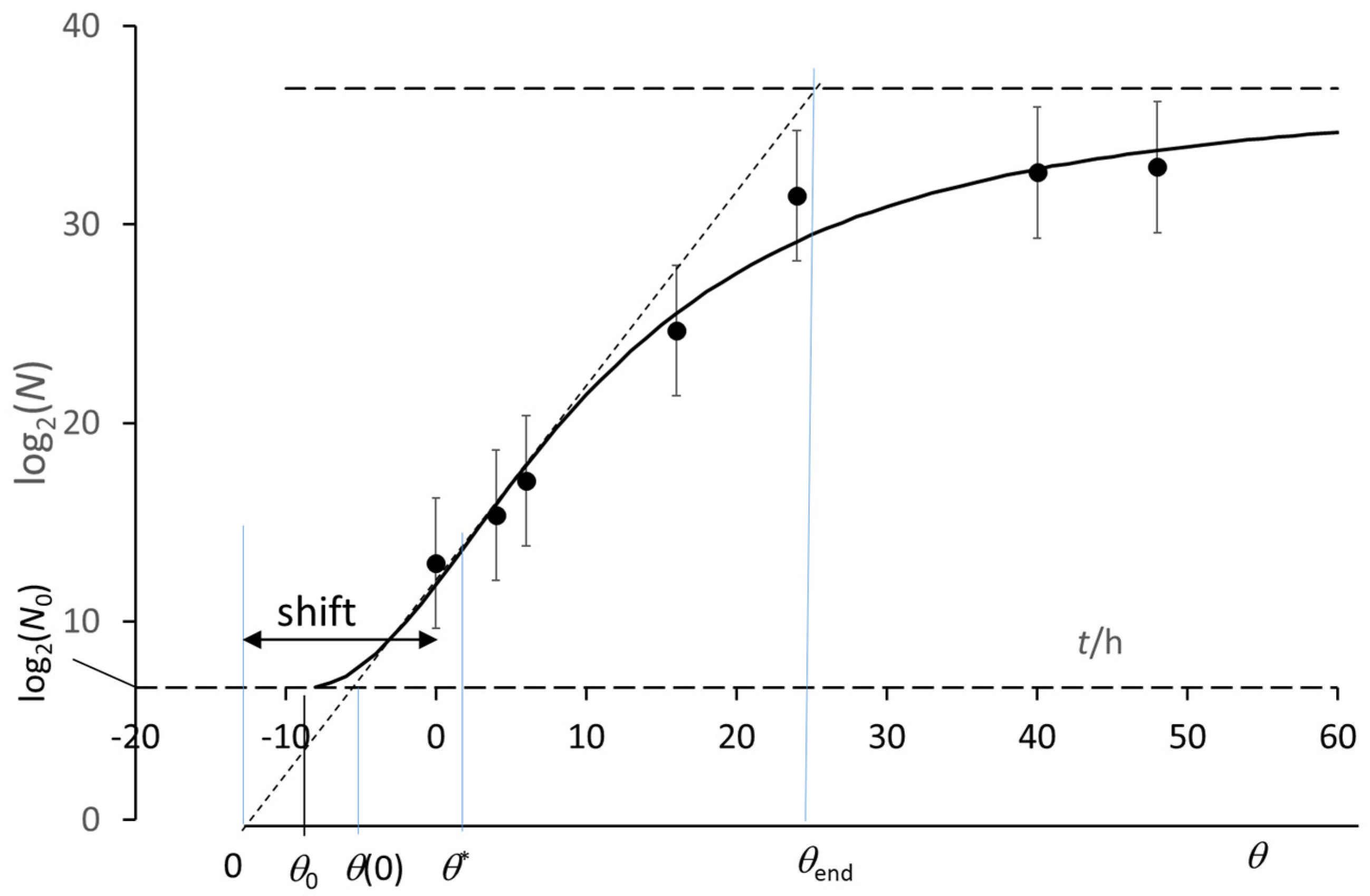
3. The Growth Curve: The Result of an Auto Correlation Effect

The message of Figure 4 is that the value of the duplication pace directly depends on the number of duplication steps experienced by the cells of the virtual culture. With reference to Figure 2 and after Equation (6), the time-dependent pace of the pseudo autocatalytic mechanism is:

$$k\left(t\right)=2\mathrm{l}\mathrm{n}(2)\sqrt{{\displaystyle \frac{\beta }{\alpha }}}\sqrt{\xi {(1-\xi )}^3}$$

(7)

that causes the eventual steep decay of $\dot{N}$, since k(t) → 0 for ξ →1, for any value of α and β.

This interpretation is consistent with the purposely naïve assumption that N and ξ are the only variables that define the behavior of the ideal culture, not implying any hypothesis about genomic and biochemical processes at the cell level. Nonetheless, the value of the steepest slope of the real growth curve is of help to define the origin of the time scale (see below).

N = 1 matches the idea of “time origin”, θ = 0, since a necessary condition to start the duplication in any given volume unit of the culture is the presence of one cell. In the log(N)-vs-t plot, one can extrapolate the tangent straight line at the steepest point of the growth curve down to log(N) = 0 (no matter the log base) and identify the time origin θ = 0 as its intercept with the time axis. This does not necessarily coincide with t = 0, corresponding to either a positive or a negative value of t (Figure 5). The experimental data collected for θ < 0 (normally, with values not significantly different from N₀) would reflect either some experimental mistake [20,32] or metabolic activities that do not deal with the preparation of the duplication process [15].

This approach aims to connect the behavior of the real culture with that of the virtual one where duplication is the only process to occur. The straight-line trend would indeed reflect a duplication process that can progress at the maximum rate, meeting no adverse effect. In the log₂(N)-vs-θ plot, the steepest slope of the growth curve is $\mu ={\displaystyle \frac{3\sqrt{3}}{8}}\sqrt{{\displaystyle \frac{\beta }{\alpha }}}$ and the equation for the tangent straight line is as follows:

$$\mu \theta ={log}_2\left(N\right),$$

(8)

with

• $\mu \theta (0)={log}_2\left(N_0\right)$ and
• $\mu {\theta }^{\mathrm{*}}={log}_2\left(N_0\right)+\beta /4$ and
• $\mu {\theta }_{end}={log}_2\left(N_0\right)+\beta$

The following was recognized [29,30]:

• (θ* − θ_end) = 2(θ* − θ₀),
• [θ* − θ(0)] = 2 [θ(0) − θ₀],

with θ₀ as the onset point of the duplication process that mimics the growth curve. For θ = θ₀, the ideal straight line crosses the level [log₂(N₀) − β/8]. Figure 5 reports the application of the above expressions.

This means that the variable “t” in the Equations (1)–(4) actually stands for the difference (θ − θ₀), and θ₀ is the third adjustable parameter of the model. The value of θ₀ is the duration of the duplication latency that precedes the onset of the duplication process and therefore conceptually differs from the lag phase λ described by other authors [5,9,15,17], as it is consistent with the duplication parameters, α and β, and related to an independent (θ = 0 for N = 1) time origin.

No matter the time origin, every growth curve that is the result of a duplication process obeys the “linearization” as follows:

$${log}_2\left({\displaystyle \frac{N}{N_0}}\right)=\beta \xi ,$$

(9)

where ξ is the independent variable, with ξ = 0 for θ = θ₀. The ideal straight line stemming from the origin θ = 0 with slope μ is as follows:

$${log}_2\left(N\right)=\mu \theta ={log}_2\left(N_0\right)+\mu \left[\theta -\theta (0)\right],$$

(10)

which implies that the condition N = 1 for θ = 0 formally corresponds to a peculiar ξ value (Figure 6) as in the following equation:

$${\xi }_{N=1}=-{\displaystyle \frac{\mu \theta (0)}{\beta }}={\displaystyle \frac{{\left[{log}_2\left({N/N}_o\right)\right]}_{N=1}}{\beta }}$$

(11)

This means that the time origin singled out by extrapolating the tangent to the growth curve at its steepest (flex) point reflects a condition strictly related to the values of the main parameters that allow for the best fit of the experimental data. In other words, the growth curve of the virtual culture implies a self-consistency between the time origin and its own fitting parameters. This constraint holds for every log(N)-vs-t growth curve with a sigmoid shape and a flex point, reproduced with the present model, no matter the underlying genomic/biochemical peculiarities of the relevant microbial culture (cells + medium).

Since the duplication pace, (1/τ), of the virtual culture depends only on the attained duplication step, ξ, (see Figure 4), the overall duplication progress depends on its own progress degree; this looks like the effect of an autocorrelation. In this perspective, all the growth curves of the real microbial cultures reproduced with the present model may be referred to as the result of the same kind of autocorrelation, as any genomic, biochemical, and physical peculiarity is “translated” to an effect of the degree of progress of the corresponding virtual culture. Equation (9) is therefore a master equation that reflects every growth curve.

Figure 7 reports the same case study as Figure 5.

The sigmoid shape of the growth curve in the log(N)-vs-t plot depends on the fact that the early progress of the population density implies an increase in N that does not substantially change its order of magnitude (Figure 1) and therefore poorly affects the duplication pace. This is why the starting onset of the growth curve is rather mild. The maximum of the duplication rate, $\dot{N}$, occurs when the process is not far from its end (Figure 4), while the eventual drop of $\dot{N}$ depends on the corresponding almost naught value of (1/τ) (Figure 4).

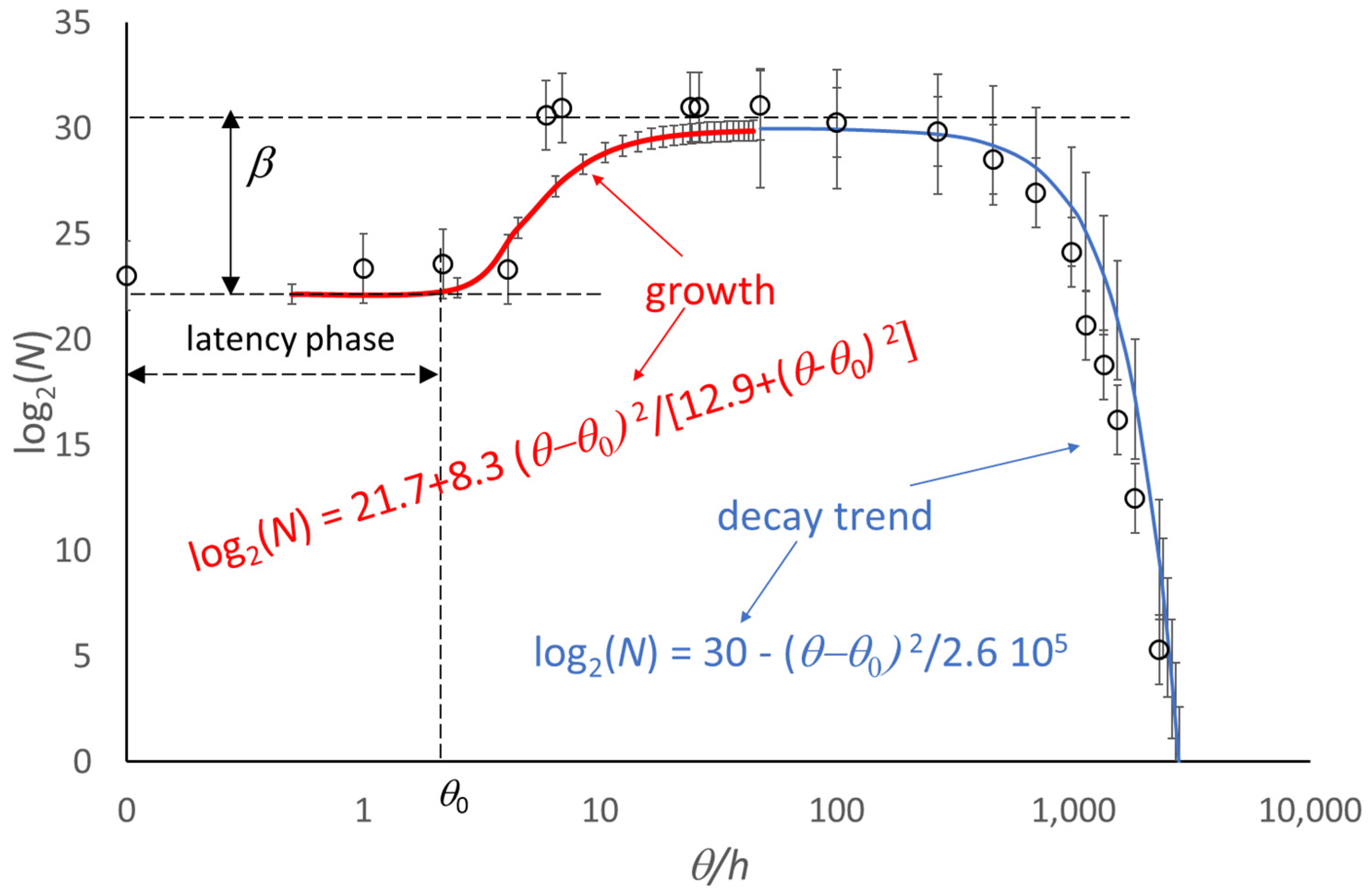
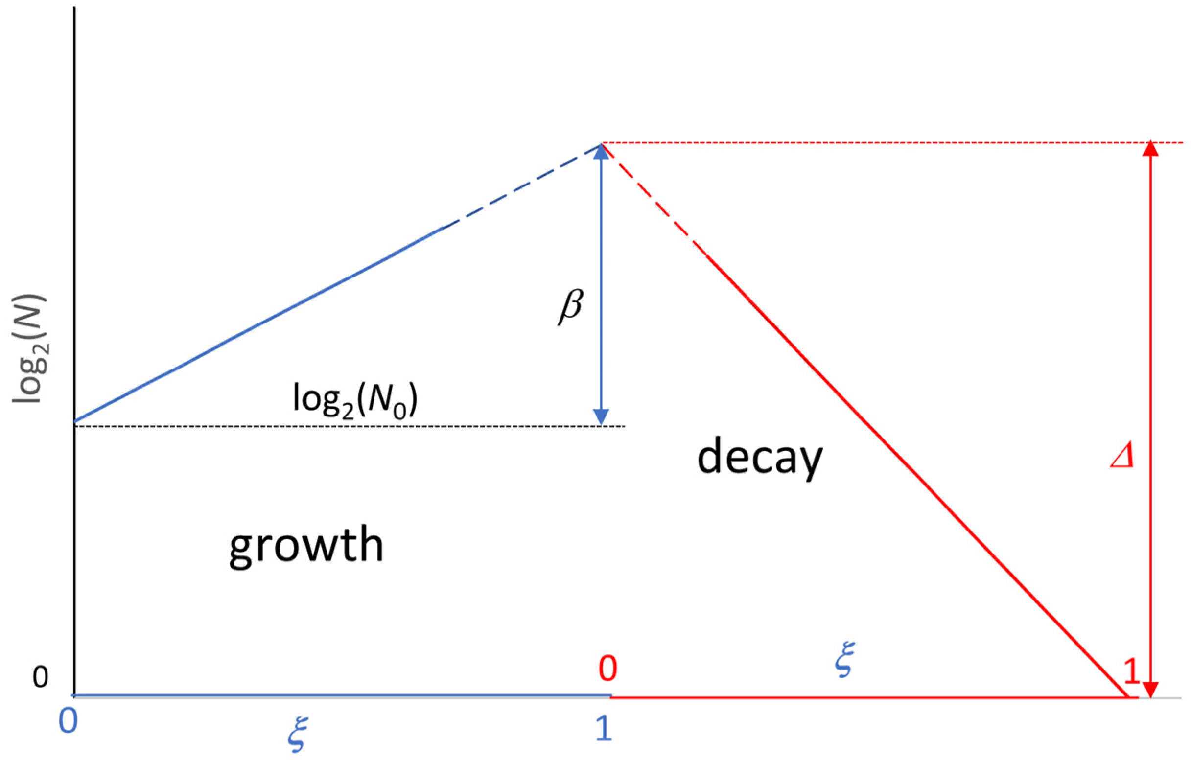
4. Extension of the Model to the Decay Phase

In the virtual culture described by this model, duplication is the only process during the growth phase. The starting population, N₀, hosts cells of the same age, while the increase in the cell population implies the appearance of cells of different ages. If one assumes that age and detrimental changes in the medium, which occurred during the growth process, are responsible for the decay in the microbial population, the first cells to die are the oldest ones.

Ranking the microbial population of the virtual culture according to the age of the cells born in the different duplication steps allows one to recognize [29] that, at the end of the growth process, the number of the oldest cells, namely those born in the early duplication steps, is practically negligible with respect to that of the youngest ones. This is why the start of the decay can look like a log(N) plateau that precedes the eventual steep decline of the microbial population; this is a fake view related to the use of a log scale for the population density. However, the literature has reported case studies where the growth phase goes through a broad maximum of log(N) [34,35]. Both situations can be reproduced by assuming a pseudo exponential decay trend with a decreasing decay time, τ_d = δ/(θ − θ_S), to account for the observed decay acceleration. The population density for θ ≥ θ_S is as follows:

$$N_{\theta \ge {\theta }_s}=N_0{2}^{\beta -{\displaystyle \frac{\mathsf{\Delta }{(\theta -{\theta }_S)}^2}{\delta +{(\theta -{\theta }_S)}^2}}}$$

(12)

where θ_S, Δ, and δ are parameters that come from the best fit of experimental data collected during the decay phase of the real microbial culture (Figure 8).

This approach aims to describe the decay phase of the virtual microbial culture, including the almost steady value of log(N) attained at the end of the growth, as due to the exhaustion of the life span for cells born in the different duplication steps [29,30]. The final cascade decay trend would mainly occur because of the much larger number of cells born in the final generation steps of the growth phase. The overall decay trend looks like a reverse of the growth trend, as far as it affects one-by-one (ξ is the corresponding scanning parameter) each generation steps in the same order as in the preceding growth phase,

$$N=N_0{2}^{\beta -\xi \mathsf{\Delta }},$$

(13)

with $\mathsf{\Delta }=\beta -{\left[{log}_2\left({\displaystyle \frac{N}{N_0}}\right)\right]}_{N=1}$ and $\xi ={\displaystyle \frac{{(\theta -{\theta }_S)}^2}{\delta +{(\theta -{\theta }_S)}^2}}$. In the log(N)-vs-ξ plot, Equation (13) corresponds to a straight line, although with a steeper slope, as the decay end level is N = 1 (Figure 9). The use of ξ as an independent variable conceals any time gap between growth and the decay trends that converge to an intermediate point.

It is worth noticing that the above decay function (Equation (12)) does not apply to cases where the microbial population reacts to the adverse conditions that accompany the decay with peculiar physiologic adjustments, like sporulation and endo-cellular biochemical changes [28].

5. Use of the Model

This approach suggests the need of an accurate routine to treat the experimental data, which includes the following:

• identify the time origin θ = 0 by extrapolating the straight-line tangent to the experimental growth at its steepest point down to log(N) = 0 (no matter the log base);
• adjust the time scale;
• discard all data that correspond to negative θ;
• use only the remaining data that are significantly above the value of N₀;
• use the equation ${\log }_2\left({\displaystyle \frac{N}{N_0}}\right)={\displaystyle \frac{\beta {(\vartheta -{\theta }_0)}^2}{\alpha \beta +{(\vartheta -{\theta }_0)}^2}}$ (or equivalent for other log bases) for the best fit.

The model is easy to use and offers the following advantages:

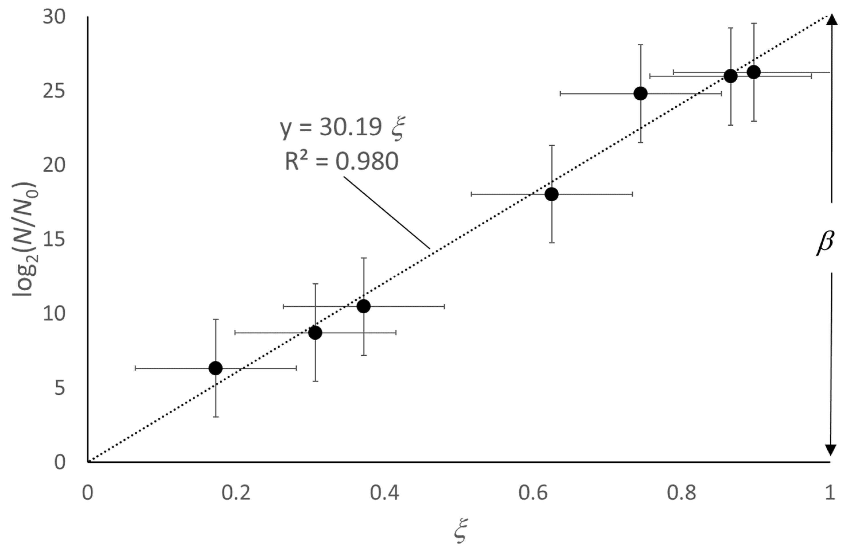
• It provides an ideal and common reference behavior for every microbial culture; the comparison between different growth curves of real microbial cultures simply requires a check of the values of α, β, and θ₀. The effects observed by varying the conditions of a given microbial culture (starting population density, temperature, pH, kind of substrate, water activity, etc.) produce a quantitative response in different values of α, β and θ₀. This can be of help in predictive microbiology investigations.
• Although based on the best fit of the growth curve in the log(N)-vs-t format, the model applies to the natural N-vs-t scale, as it defines an ideal trend related to a time origin, θ = 0, where N = 1.
• A naked-eye analysis of the experimental growth curve allows for a tentative identification of its steepest point, a tentative drawing of the tangent to the growth curve, and a tentative location of the time origin for the ideal culture, which allow some quick qualitative predictions. One can perfect this approach through iterative best fits with the normal time scale in order to identify t* and quantify the slope of the straight-line tangent to the experimental growth curve and adjust the assessment of the origin of the time scale for the virtual microbial culture.
• Finally, the model also holds for the decay phase of a real microbial culture, thanks to the assumption that the oldest cells are the first to die. This also allows for the description of the complete growth-and-decay trend with a single function [28,29,30].

6. Conclusions

A purposely naïve and semi-empirical model allows for the reproduction of the phenomenological behavior of any real microbial culture by adjusting the values of three parameters, α, β and θ₀, which have a biological meaning only for the virtual microbial culture that mimics the behavior of the real ones. In such an ideal situation, β is the maximum number of duplication steps for the generation lines stemming from the starting N₀ population, (β/α)^1/2 is proportional to the overall duplication rate, and θ₀ reflects the promptness of the culture to undertake the duplication process.

Any genomic, biochemical, and physical peculiarity (microbial species, physiological condition, pH, water activity, temperature, etc.) that distinguishes one real culture from another is “translated” to an effect of the progress degree of the population density, ξ, and cell age in the virtual culture that closely mimics the trend of the experimental data. In this perspective, growth, and decay of the microbial population show trends that seem to be the result of an autocorrelation represented by Equation (9) and Equation (13), respectively.

This view justifies the observed sigmoid shape of the growth curves in the traditional the log(N)–vs–t plot.

A further support of the present model comes from the realization that β is also a reasonable proxy of the culture fitness, which complies with a thermodynamic perspective [31] of the evolution of a microbial culture in a Long-Term Evolution Experiment.

References

1. Neidhardt, F.C. Bacterial growth: Constant obsession with dN/dt. J. Bacteriol. 1999, 181, 7405–7408. [Google Scholar] [CrossRef]
2. Lopez, S.; Prieto, M.; Dijkstra, J.; Dhanoad, M.S.; France, J. Statistical evaluation of mathematical models for microbial growth. Int. J. Food Microbiol. 2004, 96, 289–300. [Google Scholar] [CrossRef] [PubMed]
3. Antolinos, V.; Muñoz-Cuevas, M.; Ros-Chumillas, M.; Periago PMFernández, P.S.; Le Marc, Y. Modelling the effects of temperature and osmotic shifts on the growth kinetics of Bacillus weihenstephanensis in broth and food products. Int. J. Food Microbiol. 2012, 158, 36–41. [Google Scholar] [CrossRef] [PubMed]
4. Mellefont, L.A.; McMeekin, T.A.; Ross, T. Effect of relative inoculum concentration on Listeria monocytogenes growth in co-culture. Int. J. Food Microbiol. 2008, 121, 157–168. [Google Scholar] [CrossRef] [PubMed]
5. Baranyi, J.; George, S.M.; Kutalik, Z. Parameter Estimation for the Distribution of Single Cell Lag Times. J. Theor. Biol. 2009, 259, 24–30. [Google Scholar] [CrossRef] [PubMed]
6. Gime’nez, B.; Dalgaard, P. Modelling and predicting the simultaneous growth of Listeria monocytogenes and spoilage micro-organisms in cold-smoked salmon. J. Appl. Microbiol. 2004, 96, 96–109. [Google Scholar] [CrossRef]
7. Vadasz, P.; Vadasz, A.S. Biological implications from an autonomous version of Baranyi and Roberts growth model. Int. J. Food Microbiol. 2007, 114, 357–365. [Google Scholar] [CrossRef]
8. Baranyi, J.; Pin, C. Estimating Bacterial Growth Parameters by Means of Detection Times. Appl. Environ. Microbiol. 1999, 65, 732–736. [Google Scholar] [CrossRef]
9. Baranyi, J.; Pin, C.; Ross, T. Validating and comparing predictive models. Int. J. Food Microbiol. 1999, 48, 159–166. [Google Scholar] [CrossRef]
10. Buchanan, R.L.; Whiting, R.C.; Damert, W.C. When is simple good enough: A comparison of the Gompertz, Baranyi, and three-phase linear models for fitting bacterial growth curves. Food Microbiol. 1997, 14, 313–326. [Google Scholar] [CrossRef]
11. Swinnen, I.A.M.; Bernaerts, K.; Dens, E.J.J.; Geeraerd, A.H.; Van Impe, J.F. Predictive modelling of the microbial lag phase: A review. Int. J. Food Microbiol. 2004, 94, 137–159. [Google Scholar] [CrossRef]
12. Schaechter, M. From growth physiology to systems biology. Int. Microbiol. 2006, 9, 157–161. [Google Scholar] [PubMed]
13. Gonze, D.; Coyte, K.Z.; Lahti, L.; Faust, K. Microbial communities as dynamical systems. Curr. Opin. Microbiol. 2018, 44, 41–49. [Google Scholar] [CrossRef]
14. Good, B.H.; Hallatschek, O. Effective models and the search for quantitative principles in microbial evolution. Curr. Opin. Microbiol. 2018, 45, 203–212. [Google Scholar] [CrossRef]
15. Bertrand, R.L. Lag phase is a dynamic, organized, adaptive, and evolvable period that prepares bacteria for cell division. J. Bacteriol. 2019, 201, e00697-18. [Google Scholar] [CrossRef]
16. Scott, M.; Hwa, T. Bacterial growth laws and their applications. Curr. Opin. Biotechnol. 2011, 22, 559–565. [Google Scholar] [CrossRef] [PubMed]
17. Basan, M.; Honda, T.; Christodoulou, D.; Hörl, M.; Chang, Y.u.-F.; Leoncini, E.; Mukherjee, A.; Okano, H.; Taylor, B.R.; Silverman, J.M.; et al. A universal trade-off between growth and lag in fluctuating environments. Nature 2020, 584, 470–474. [Google Scholar] [CrossRef] [PubMed]
18. Dens, E.J.; Bernaerts, K.; Standaert, A.R.; Van Impe, J.F. Cell division theory and individual-based modeling of microbial lag Part I. Int. J. Food Microbiol. 2005, 101, 303–318. [Google Scholar] [CrossRef]
19. Dens, E.J.; Bernaerts, K.; Standaert, A.R.; Kreft, J.-U.; Van Impe, J.F. Cell division theory and individual-based modeling of microbial lag Part II. Int. J. Food Microbiol. 2005, 101, 319–332. [Google Scholar] [CrossRef]
20. Atolia, E.; Cesar, S.; Arjes, H.A.; Rajendram, M.; Shi, H.; Knapp, B.D.; Khare, S.; Aranda-Díaz, A.; Lenski, R.E.; Huang, K.C. Environmental and physiological factors affecting high-throughput measurements of bacterial growth. mBio 2020, 11, e01378-20. [Google Scholar] [CrossRef]
21. Baranyi, J. Comparison of Stochastic and Deterministic Concepts of Bacterial Lag. J. Theor. Biol. 1998, 192, 403–408. [Google Scholar] [CrossRef]
22. Sutton, S. Measurement of Microbial Cells by Optical Density. J. Valid. Technol. 2011, 17, 42–46. [Google Scholar]
23. Schiraldi, A. Microbial growth in planktonic conditions. Cell Develop. Biol. 2017, 6, 1–6. [Google Scholar] [CrossRef]
24. Schiraldi, A. A self-consistent approach to the lag phase of planktonic microbial cultures. Single Cell Biol. 2017, 6, 3. [Google Scholar] [CrossRef]
25. Schiraldi, A. Growth and decay of a planktonic microbial culture. Int. J. Microbiol. 2020, 2020, 4186468. [Google Scholar] [CrossRef]
26. Schiraldi, A.; Foschino, R. An alternative model to infer the growth of psychrotrophic pathogenic bacteria. J. Appl. Microbiol. 2022, 132, 642–653, (and related “Supporting Information”). [Google Scholar] [CrossRef]
27. Schiraldi, A.; Foschino, R. Time scale of the growth progress in bacterial cultures: A self-consistent choice. RAS Microbiol. Infect. Dis. 2021, 1, 1–8. [Google Scholar] [CrossRef]
28. Schiraldi, A. Batch Microbial Cultures: A Model that can account for Environment Changes. Adv. Microbiol. 2021, 11, 630–645. [Google Scholar] [CrossRef]
29. Schiraldi, A. The Origin of the Time Scale: A Crucial Issue for Predictive Microbiology. J. Appl. Environ. Microbiol. 2022, 10, 35–42. [Google Scholar] [CrossRef]
30. Schiraldi, A. The growth curve of microbial cultures: A model for a visionary reappraisal. Appl. Microbiol. 2023, 3, 288–296. [Google Scholar] [CrossRef]
31. Schiraldi, A. The growth of microbial cultures complies with the laws of thermodynamics. Biophys. Chem. 2024, 307, 107177. [Google Scholar] [CrossRef] [PubMed]
32. Egli, T. Microbial growth and physiology: A call for better craftsmanship. Front. Microbiol. 2015, 6, 287–298. [Google Scholar] [CrossRef] [PubMed]
33. Fessas, D.; Schiraldi, A. Isothermal calorimetry and microbial growth: Beyond modeling. J. Therm. Anal. Calorim. 2017, 130, 567–572. [Google Scholar] [CrossRef]
34. Doona, C.J.; Feeherry, F.E.; Ross, E.W. A quasi-chemical model for the growth and death of microorganisms in foods by non-thermal and high-pressure processing. Int. J. Food Microbiol. 2005, 100, 21–32. [Google Scholar] [CrossRef] [PubMed]
35. Peleg, M. A Model of Microbial Growth and Decay in a Closed Habitat Based on Combined Fermi’s and the Logistic Equations. J. Sci. Food Agric. 1996, 71, 225–230. [Google Scholar] [CrossRef]
Figure 1. Growth curve. Comparison of natural and log scales for the values of the population density.
Applmicrobiol 04 00086 g001
Figure 2. A naïve duplication process looks like a branching chain process of pseudo autocatalytic cycles with a time-dependent pace, k(t).
Applmicrobiol 04 00086 g002
Figure 3. Trends of duplication pace, 1/τ, duplication rate, N ˙ , and “specific duplication rate”, ( N ˙ N ) . The values of the parameters used to draw these trends are typical for the best fit of data from real microbial cultures, namely N0 = 104 CFU/mL, α = 0.5 (time units2) and β = 10. The scales of the axes are in arbitrary units.
Applmicrobiol 04 00086 g003
Figure 4. Trends of 1/τ, log2(N/N0) and N ˙ versus the reduced variable ξ = log2(N/N0)/β. The former goes through a broad maximum around ξ = 0.5 for any value of β, while the position of the maximum N ˙ depends on β (for β = 10 and 20, it occurs at ξ = 0.876 and 0.933, respectively).
Applmicrobiol 04 00086 g004
Figure 5. Extrapolation of the straight-line tangent to the experimental growth curve (circles, Lactobacillus helveticus [33] at its steepest point down to the level log(N) = 0 to identify the time origin θ = 0 for the virtual culture that replaces the time origin “t = 0” for the experimenter. Bars correspond to the standard error.
Applmicrobiol 04 00086 g005
Figure 6. Linearization of the growth curve (heavy red line, Equation (9)) and comparison with the straight line (blue dotted line, Equation (10)) that singles out the time origin, θ = 0 for N = 1 (see text). The duration of the pre-duplication latency, θ0, is equal to μθ(0)/β in ξ units. Red and blue letters refer to log2(N/N0)-vs-ξ and log2(N)-vs-θ plots, respectively. Equation (4) indicates that ξ → 1 for θ →∞.
Applmicrobiol 04 00086 g006
Figure 7. Linearized growth curve for the same case study as in Figure 5. The ξ values come from Equation (4) after replacing t with (θθ0). Bars correspond to the standard error.
Applmicrobiol 04 00086 g007
Figure 8. Growth and decay trend of a culture of Escherichia coli. data from Combase. Because of the width of the time range considered, θ is in log10 units. Bars correspond to standard error. Modified from ref. [28].
Applmicrobiol 04 00086 g008
Figure 9. Linearized growth and decay cycle in the log2(N)-vs-ξ plot.
Applmicrobiol 04 00086 g009
Disclaimer/Publisher’s Note: The statements, opinions and data contained in all publications are solely those of the individual author(s) and contributor(s) and not of MDPI and/or the editor(s). MDPI and/or the editor(s) disclaim responsibility for any injury to people or property resulting from any ideas, methods, instructions or products referred to in the content.