Classification of Verticillium dahliae Vegetative Compatibility Groups (VCGs) with Machine Learning and Hyperspectral Imagery

Abstract

Vegetative compatibility groups (VCGs) in fungi like Verticillium dahliae are important for understanding genetic diversity and for informed plant disease management. This study utilized hyperspectral imagery (HSI) and machine learning to differentiate the VCGs of V. dahliae. A total of 194 isolates from VCGs 2B and 4A and 4B were cultured and imaged across the 533–1719 nm spectral range, and the spectral, textural, and morphological features were extracted. The study documented the spectral profiles of V. dahliae’s isolates and identified specific spectral features that can effectively differentiate among the VCGs. Multiple machine learning algorithms, including random forest and artificial neural networks (ANNs), were trained and evaluated on previously unseen isolates. The results showed that combining spectral, textural, and morphological data provided the highest classification accuracy. The ANN model achieved a 79.4% accuracy overall, with an 87% accuracy for VCG 2B and 88% for VCG 4A, but it had consistently low accuracies for VCG 4B. Although this work utilized only three of the nearly eight known VCGs, the findings underscore the potential of the HSI for fungal group classification. The study also highlights the need for future work to include a wider range of VCGs from multiple regions, larger sample sizes, and careful selection of feature sets to enhance model performance and generalizability.

1. Introduction

Self/nonself recognition is common in filamentous fungi [1]. Fungi distinguish self from nonself mycelium and only form stable heterokaryons with individuals that share similar genetics [2,3]. Fungi that form stable heterokaryons are grouped into vegetative compatibility groups (VCGs), anastomosis groups, mycelial compatibility groups, or somatic compatibility groups [3]. Multiple alleles at heterokaryon incompatibility (het) loci regulate heterokaryon incompatibility in fungi [4,5]. Hyphal fusion of non-allelic strains results in compartmentalization and cell death [3]. Although fungal anastomosis is required to introduce genetic diversity, several filamentous fungi, including Neurospora crassa, Aspergillus nidulans, Verticillium dahliae, and Fusarium oxysporum, may use this phenomenon to limit the exchange of harmful viruses, plasmids, cell organelles, or dominance by aggressive isolates [6,7,8,9,10]. Moreover, heterokaryon incompatibility is essential for the survival and maintenance of the unique population of fungi [11].

Knowledge about the prevalence and distribution of vegetative compatibility groups also informs the genetic structure and diversity within fungal species. Several studies have detected correlations between VCGs and distinct clonal lineages with molecular tools in several plant pathogenic and endophytic fungi including Verticillium dahliae, Fusarium oxysporum, and Sclerotium rolfsii [12,13,14,15]. In addition, VCGs of plant pathogenic fungal species also show host-specific adaptation and virulence toward certain hosts [16,17]. Therefore, classification of VCGs is important to assess fungal diversity, study evolution, and make informed plant disease management decisions.

For example, VCGs have been used to study diversity, evolution, and inform management decisions for Verticillium wilts, caused by the asexual haploid fungus, Verticllium dahlia [18,19]. V. dahliae is an endophyte and pathogen of hundreds of plant species [20,21,22,23]. So far, at least eight VCGs have been documented in V. dahliae, namely, VCG 1A, VCG 1B, VCG 2A, VCG 2B, VCG 3, VCG 4A, VCG 4B, and VCG 6 [24,25,26,27]. Traditionally, these VCGs are differentiated with nitrate non-utilizing (nit) mutants [28]. Isolates are assigned to VCGs after complementation is observed (generally by the presence of microsclerotia) with known tester strains. Because this method is resource- and time-intensive, other methods have been pursued.

Molecular studies conducted in VCGs in the last two decades led to the development of amplified fragment length polymorphism (AFLP), microsatellite, and single nucleotide polymorphism (SNP) based molecular markers to characterize VCGs [15,29]. For example, Collado–Romero et al. [30] developed PCR markers to differentiate groups of VCGs like VCG 2A and VCG 4B, VCG 1A and VCG 2B, and VCG 4A and VCG 2B. However, robust markers that can differentiate each VCG accurately have yet to be developed [31]. To address this problem, quick and resource-frugal methods are needed to classify VCGs.

Recently, hyperspectral and multispectral imagery have gained popularity in biomedicine, food, and agricultural industries to classify diseases, anomalies, contaminations, and crops [32,33,34,35]. Several fungal and bacterial strains have been successfully distinguished at the genus and species levels using spectroscopic and hyperspectral imagery methods [36]. Most of the studies conducted in this area have used either microscopic hyperspectral imagery or spectroscopic methods for data acquisition. A limited number of studies have used macroscopic hyperspectral images to study spectral dynamics of fungal genera and species. Lu et al. [37] classified five fungal species—Aspergillus parasiticus, A. flavus, A. glaucus, A. niger, and Penicillium sp.—using macroscopic hyperspectral images with up to a 98% accuracy. Similarly, Williams et al. [38] classified three species of Fusarium—F. verticillioides, F. subglutinans, and F. proliferatum—at the macroscopic level using hyperspectral imagery. Within species, classification has also been successful. Salman et al. [39] classified VCGs of Colletotrichum coccodes with nearly 85% accuracy using spectral data obtained from infrared spectroscopy. To the best of our knowledge, no studies have used hyperspectral images to classify VCGs of fungal species.

The goal of this project was to investigate whether the VCGs of V. dahliae colonies can be differentiated using hyperspectral imagery (HSI). The objectives of the study were as follows: (i) to capture the spectral, morphological, and textural signatures of the VCGs (VCG 2B, VCG 4A, and VCG 4B) of V. dahliae in the visible, near-infrared (NIR), and short-wave infrared (SWIR) regions of the electromagnetic spectrum; (ii) to classify the VCGs of V. dahliae based on spectral, morphological, and textural features using machine learning models; and (iii) to identify the subset of the most significant wavebands that differentiate VCGs.

2. Materials and Methods

2.1. Verticillium Dahliae Isolate Preparation and Culture

A total of 194 isolates belonging to three vegetative compatibility groups (VCGs)—76 for VCG 2B, 94 for VCG 4A, and 24 for VCG 4B—were used in this study (Supplementary Figure S1). The isolates were categorized into each VCG by Dung et al. [40], with nit mutants and tester strains. The VCGs, origin, collection year, collection region, and haplotype information of each isolate can be found in Dung et al. [40]. The isolates were retrieved from a −20 °C freezer and recovered in NP-10 medium A four mm diameter plug of actively growing mycelia was sub-cultured on full-strength potato dextrose agar (PDA)medium The volume of PDA in each plate was made uniform by dispensing 26 mL of PDA in each Petri dish using a PDA dispenser (Unispence, Wheaton Science Products, Vineland, NJ, USA). Each isolate had four replications, and each replication was inoculated over four consecutive days. Since imaging was conducted over four consecutive days, this ensured that all cultures were 20 days old at the time of imaging for consistency across samples. Inoculated plates were kept at room temperature (approx. 22 °C) under dark conditions for 20 days. Hyperspectral images were acquired for each isolate after removing the Petri dish cover.

2.2. Hyperspectral Image Acquisition

A push-broom-type hyperspectral imagery system (HSI) (Hyperspec extended VNIR, Headwall Photonics Inc., Fitchburg, MA, USA) (Figure 1a) was used to capture the images for each isolate. Images were obtained at a spectral range of 533 to 1719 nm with an 8.3 nm spectral resolution. The spatial resolution was 250 × 200 pixels. The samples were illuminated (visible–near infrared spectra) using a high-intensity quart tungsten halogen with a pulsed Xenon lamp (380–2500 nm, Headwall Photonics Inc., Fitchburg, MA, USA). The lamp was mounted next to the camera. A mirror inside the lamp’s frame was used to reflect the light toward the sample. Before image acquisition, the camera was calibrated following the procedure provided by the manufacturer and using Equation (1).

$$C_{x,y,\lambda }={\displaystyle \frac{R_{x,y,\lambda }-D_{x,y,\lambda }}{W_{x,y,\lambda }-D_{x,y,\lambda }}}$$

(1)

where C_x,y,λ, R_x,y,λ, D_x,y,λ, and W_x,y,λ are the calibrated image, raw image, dark reference image, and white reference image, respectively; x and y represent the spatial pixels; and λ represents spectral bands. The dark reference image was taken by covering the lens with the cap, whereas a white reference image was obtained by scanning the white reference panel provided by the manufacturer. The image acquisition was conducted with the following settings: (i) the distance between the lens and Petri dish was set at about 0.305 m; (ii) the speed of the moving platform was set at 0.015 m·s⁻¹; and (iii) the spectrograph exposure time was set at 0.013 s.

2.3. Hyperspectral Image Preprocessing and Feature Extraction

Each raw image (hypercube) had three dimensions. The x- and y-dimensions represent the spatial resolution, and the z-axis represents the spectral resolution (Figure 1b). The dimensions of the acquired hypercube were 200 × 250 × 144. The image preprocessing and feature extraction were performed with Python (Version 3.9.0, Python Software Foundation, Wilmington, DE, USA), an open-source programming language. All captured images were initially stored in “ENVI Standard” format (NV5 Geospatial, Broomfield, CO, USA). The Python package Spectral Python (SPy) [41] was used to read the image and was converted to a 3D (3-dimensional) NumPy array format for further processing. Since image calibration was performed while capturing the image, the obtained reflectance values ranged between 0 and 1. Further, a circular mask was created using the Python library scikit-image [42] to segment the mycelium from the PDA and the Petri dish’s edges (Figure 1d). The average reflectance value was extracted from the whole colony at 144 wavebands (Figure 1e). Before the analysis, the five wavebands at the beginning or end of the mentioned spectral range were removed to reduce the potential noise, as these regions tend to have a high signal-to-noise ratio [43]. The final spectral data included the average reflectance in the range of 574.9 to 1677.3 nm wavelength.

In addition, seven textural features, namely, contrast, dissimilarity, homogeneity, energy, correlation, angular second moment (ASM), and entropy, were extracted from ten wavebands (616, 674, 716, 898, 973, 1205, 1371, 1387, 1454, and 1636 nm). The wavebands were selected from unique spectral regions (e.g., red, red edge, reflectance peaks/valleys, and water absorption bands). Furthermore, seven morphological features, namely, area, eccentricity, major axis length, minor axis length, perimeter, solidity, and compactness, were extracted from each image. The details of the textural and morphological features are presented in Supplementary Table S1. Finally, the obtained morphological, spectral, and textural features were standardized to a mean of zero and a standard deviation of one. Image preprocessing, spectral, morphological, and textural feature extraction, as well as data standardization, were conducted in Python using various packages, including NumPy, pandas, OpenCV, and scikit-image [42,44,45,46].

The spectral reflectance across the electromagnetic spectrum was visualized using a line graph, and a 95% confidence interval for the mean reflectance at each waveband was computed via bootstrapping by calculating the 2.5th and 97.5th percentiles to define the interval’s lower and upper bounds. Also, textural and morphological features were visualized using boxplots.

The dataset was split into training and test sets based on the isolate name, with 70% of the isolates assigned to the training set and the remaining 30% assigned to the test set, while maintaining the class balance. After splitting, the training set consisted of 497 samples, and the test set consisted of 218 samples. None of the isolates in the training set were included in the test set.

2.4. Dimensionality Reduction and Feature Selection

The extracted features are high-dimensional and exhibit a high degree of correlation with one another. Two new feature datasets were derived using principal component analysis (PCA), an unsupervised machine learning method, projects new dimensions in the directions that capture the maximum variance in the data [47]. The newly derived features for each sample were visualized using a biplot. In addition, the top 15 wavebands that can differentiate the VCGs were selected using the least absolute shrinkage and selection operator (LASSO) algorithm on the training set. LASSO is based on linear regression with “l1” regularization and shrinks the linear regression coefficients to values near zero or exactly zero [47]. Features with the highest absolute coefficients were considered the most important. Hyperparameter tuning for lambda (λ) was performed, and the “λ” value yielding the highest accuracy in the training dataset through grid-search cross-validation was used for the feature selection. All feature reduction and data visualization tasks were performed in Python using the scikit-learn and seaborn packages [48,49].

2.5. Machine Learning Models Fitting and Prediction

Four supervised classical machine learning classifiers—linear discriminant analysis (LDA), support vector machine (SVM), random forest (RF), and k-nearest neighbor (kNN)—were used for model fitting and prediction using handcrafted features. Different combinations of features were trained separately and in combination to predict the VCGs. These datasets included spectral features (n = 134), morphological features (n = 7), and textural features (n = 70) extracted from the whole colony, a combination of these features (n = 211), and the top 15 spectral features (n = 15) obtained through LASSO-based feature selection. In addition, a separate analysis was conducted to evaluate the classification accuracy of the two groups (VCG 2B and VCG 4A) individually, while combining the remaining isolates into a single category. Hyperparameter tuning using the grid-search cross-validation method was performed for the SVM (C value and kernel type: rbf, poly, and linear), random forest (number of trees), and kNN (number of neighbors) on the training set. Similarly, for the artificial neural network (ANN)-based model, different types and combinations of extracted features, as described above, were used as inputs during training. A single-layer ANN architecture with 90 neurons and a ReLU activation function with 200 epochs was implemented. Furthermore, a Softmax activation function was used in the output layer, and the model was optimized using the Adam optimizer. The parameters were selected based on empirical testing of different combinations and to balance the model’s complexity and computational efficiency.

All model evaluation metrics were calculated on previously unseen isolates in the test set. Accuracy, precision, recall, and F1 scores were used as evaluation metrics to compare the performance of the different classifiers, calculated using Equations (2), (3), (4), and (5), respectively.

$$Accuracy={\displaystyle \frac{TP+TN}{TP+FP+FN+TN}}$$

(2)

$$Precision={\displaystyle \frac{TP}{TP+FP}}$$

(3)

$$Recall={\displaystyle \frac{TP}{TP+FN}}$$

(4)

$$F1score=2\times {\displaystyle \frac{Recall\ast Precision}{Recall+Precision}}$$

(5)

where TP, TN, FP, and FN stand for true positive, true negative, false positive, and false negative, respectively. Finally, classification accuracies for each VCG in the test set were calculated using the best-performing random forest model and ANN based on the evaluation metrics. All classification tasks for machine learning classifiers were implemented using the scikit-learn package in Python [48]. The TensorFlow framework in Python was used to implement artificial neural networks.

3. Results

3.1. Spectral, Textural, and Morphological Features

The average reflectance from the whole colony was extracted for the three VCGs at 134 wavelengths. The reflectance values presented in Figure 2 were normalized to a 0 to 1 scale. While the reflectance patterns across the electromagnetic spectrum were similar for all groups, the magnitude of the reflectance varied. In general, differential reflectance was observed for VCG 4A compared to VCG 2B and VCG 4B. VCG 4A had a lower overall reflectance compared to VCG 2B and VCG 4B. There was a wide 95% confidence interval for VCG 4B, with considerable overlap with the confidence interval of VCG 2B. However, no overlap in confidence intervals was observed between VCG 4A and the other VCG groups. There are no major visible reflectance peaks or valleys for the spectra from 600 to 950 nm (Figure 2). Two distinct reflectance peaks were observed in the SWIR region, the first at around 1070 nm and the second at approximately 1280 nm. No major reflectance peaks were observed in the visible (VIS) range, with only a few minor reflectance peaks occurring in the short-wave infrared (SWIR) region. Also, two reflectance valleys were observed at around 950 nm and 1200 nm. Additionally, a sharp reflectance valley was also observed at 1450 nm for VCG 2B and VCG 4B.

In addition to the spectral data, image-based textural and morphological variables were obtained and visualized for all VCGs (Supplementary Figure S2). A subset of the textural features extracted at a waveband of 1205 nm (n = 7) (Supplementary Figure S2a) and all extracted morphological features (n = 7) (Supplementary Figure S2b), both standardized, were visualized using boxplots to assess variations across VCGs. Among the textural features, VCG 4A exhibited higher variability for ASM, correlation, energy, entropy, and homogeneity compared to the other VCGs, while VCG 2B showed lower variability for most textural features. VCG 4A generally displayed a magnitude difference in standardized values for most of the textural features (contrast, dissimilarity, entropy, and homogeneity) similar to the spectral features when compared to the other two VCGs. For morphological features, VCG 4A had the highest variability across most features, indicating greater heterogeneity and more diverse structural characteristics within the group. The median values for solidity and compactness were similar across all groups, but VCG 4A had significantly higher variability. Other morphological features, such as area, eccentricity, and axis lengths, showed comparable median values among the groups, but VCG 4A displayed greater variability compared to VCG 2B and VCG 4B.

Variation among the replicates within the isolates was quantified as the standard deviation of the standardized data for the 16 selected features representing the spectral, textural, and morphological characteristics. VCG 2B consistently exhibited lower variability within isolates across most features, while VCG 4A displayed greater variation (Supplementary Figure S3).

3.2. Dimension Reduction

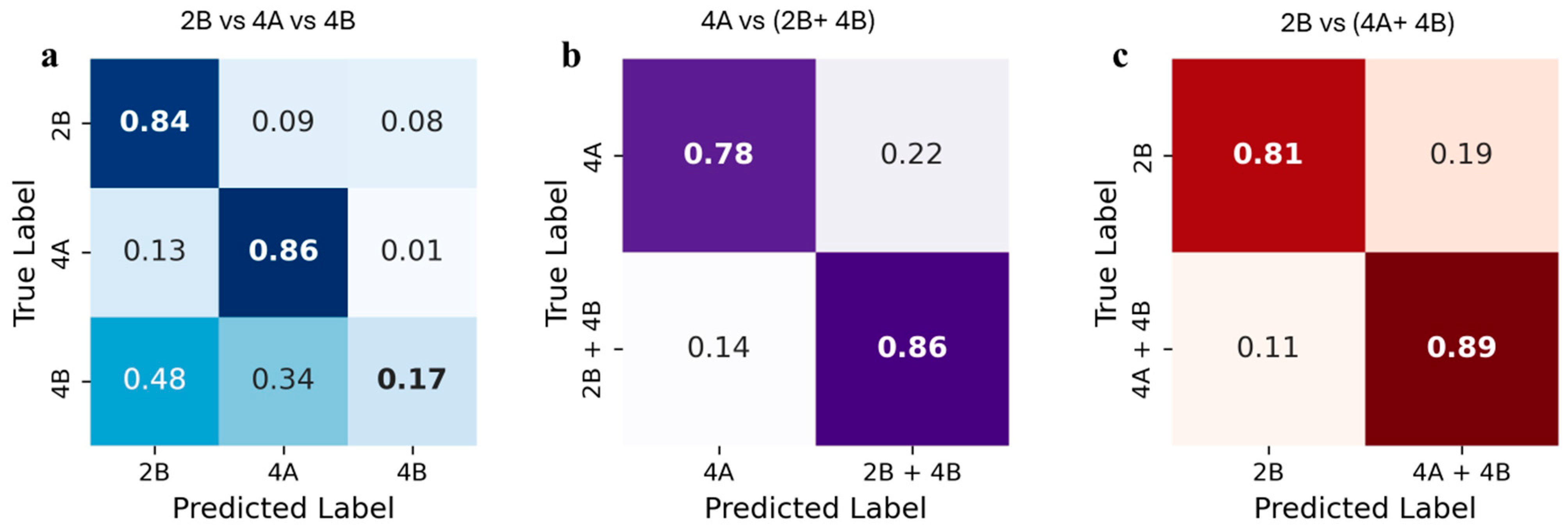
Since the obtained features are high-dimensional data, PCA was used to transform these data into lower dimensions. The new features were visualized using a biplot, where closer points indicate a higher similarity among samples (Supplementary Figure S4). The first two components of PCA explained 98.0%, 82.43%, 83.4%, and 85.62% of the variance in the original datasets containing only spectral features, textural features, morphological features, as well as a combination of all three features (Supplementary Figure S4a–d, respectively. Overall, PCA showed no clear separation of the VCGs for all data types; however, spectral features displayed relatively better clustering, with some overlap between VCG 2B and VCG 4B. Additionally, the PCA revealed more variation within VCG 4A compared to the other groups.

LASSO was implemented to identify the top 15 features for VCG separation from a spectral dataset containing 134 features. The coefficients of a total of 117 variables were shrunk to zero, while the selected features had non-zero estimated coefficients. The selected subset of features, which represented nearly 10% of the entire spectrum, included reflectance at 575, 824, 1047, 1056, 1271, 1279, 1288, 1296, 1304, 1313, 1321, 1329, 1337, 1346, and 1603 nm. Out of the 15 selected features, ten were in the 1270 to 1350 nm range, indicating the potential importance of this region in discriminating the VCGs based on spectral reflectance.

3.3. Classification

For the spectral features, a total of 134 features, as well as a subset of 15 features obtained through feature selection using LASSO, were used to classify the VCGs. Five models (LDA, RF, SVM, k-NN, and ANN) were implemented for the classification task. Among the four classical machine learning classifiers, random forest achieved the highest prediction accuracy of 76.1% on both the full reflectance and the selected subset (values bolded). The same trend was observed, in most cases, for the other evaluation metrics, for example, precision (65.6% for full and 69.4% for the subset), recall (62.4% for full and 63.5% for the subset), and F1 score (62.1% for full and 63.6% for the subset) (

Table 1. Classification accuracy, precision, recall, and F1 score obtained on the test set for five machine learning classifiers. A total of 134 spectral features and total of 15 selected spectral features obtained using LASSO were used to train all classifiers.

Model	All Spectral Features (n = 134)				Selected Spectral Features (n = 15)
	Accuracy	Precision	Recall	F1 Score	Accuracy	Precision	Recall	F1 Score
LDA	0.693	0.603	0.606	0.597	0.739	0.644	0.597	0.581
RF	0.761	0.656	0.624	0.621	0.761	0.694	0.635	0.636
SVM	0.706	0.545	0.548	0.539	0.679	0.622	0.629	0.613
k-NN	0.729	0.817	0.571	0.539	0.734	0.711	0.583	0.561
ANN	0.711	0.560	0.570	0.548	0.734	0.613	0.593	0.577

). The details of the evaluation metrics for all classifiers and both sets of spectral datasets are presented in Table 1.

At the class level, the highest accuracy was observed for VCG 4A (86%), followed by VCG 2B (84%) and VCG 4B (17%) (Figure 3a), for both sets of spectral datasets using the best-performing random forest model. VCG 4B was mostly misclassified as both VCG 2B and VCG 4A, with a higher proportion as VCG 2B (Figure 3a). The model showed higher robustness in distinguishing between VCG 2B and VCG 4A. Therefore, further analysis was conducted to evaluate the classification accuracy of each group individually, while combining the remaining isolates into a single category. VCG 4A achieved an accuracy of 78%, while the combined isolates were classified with an 86% accuracy (Figure 3b). Similarly, VCG 2B achieved an accuracy of 81% when the rest of the isolates were grouped together (Figure 3c).

In addition, the morphological, textural, and combined spectral, morphological, and textural features were trained and tested separately to identify the set of features with the highest predictability; the evaluation metrics are reported in Supplementary Table S2. The models performed variably in classifying the VCG groups across the various datasets. None of the models consistently outperformed the others in terms of all of the evaluation metrics for the textural and morphological features, while the ANN was consistently superior across all metrics for the high-dimensional combined dataset. The highest classification accuracy was achieved with LDA and k-NN for the textural dataset, achieving a 78.0% accuracy, and with random forest for the morphological dataset, achieving a 65.6% accuracy. The highest F1 score was observed with LDA for the textural dataset and SVM for the morphological dataset. The combined dataset achieved an accuracy of 79.4% and an F1 score of 70.5% using the ANN. Overall, the dataset combining the morphological, textural, and spectral features resulted in a better performance than the datasets containing only one type of feature.

The classification accuracies were calculated for the VCGs of the different data types and are presented in

Table 2. Classification accuracies for VCG 2B, VCG 4A, and VCG 4B on the test datasets using random forest and artificial neural network (ANN) models for three different datasets.

Dataset	Classifier	Vegetative Compatibility Groups (VCGs)
		2B	4A	4B
Textural (n = 70)	RF	0.89	0.87	0.03
	ANN	0.78	0.84	0.28
Morphological (n = 7)	RF	0.71	0.79	0.00
	ANN	0.82	0.75	0.00
Combined (Spectral + Textural + Morphological) (n = 211)	RF	0.91	0.88	0.17
	ANN	0.87	0.88	0.28

. For the textural dataset, RF achieved accuracies of 89% and 87% in classifying VCG 2B and VCG 4A, respectively, while the ANN had a 78% accuracy for VCG 2B and 84% for VCG 4A. For the morphological dataset, RF exhibited a 71% accuracy for VCG 2B and 79% for VCG 4A, whereas the ANN achieved an 82% accuracy for VCG 2B and 75% for VCG 4A. With the combined dataset, RF reached 91% for VCG 2B and 88% for VCG 4A, while the ANN yielded 87% for the 2B and 88% for the 4A groups. For VCG 4B, the RF and ANN consistently showed lower accuracies across all datasets. Overall, the algorithms of the random forest and artificial neural network, using the dataset that included all handcrafted features—spectral, textural, and morphological—exhibited the highest overall and class-wise accuracies in classifying the vegetative compatibility groups of Verticillium dahliae.

4. Discussion

Accurate classification of Verticillium dahliae’s vegetative compatibility groups (VCGs) is important for understanding the genetic diversity of fungi and to implement effective disease management strategies [11,15]. The classic culture-based method is often tedious and time-consuming. Although efforts to develop molecular markers are ongoing, the results have been inconsistent, and no single marker has proven capable of differentiating all VCGs [30]. To the best of our knowledge, this is the first study to highlight the potential utility of hyperspectral imaging (HSI) combined with advanced machine learning (ML) classifiers to differentiate the VCGs (2B and 4A and 4B) of Verticillium. dahliae. This study documents the spectral profiles of genetically and geographically diverse V. dahliae cultures in the visible and shortwave infrared (SWIR) regions of the electromagnetic spectrum. Also, we identified a subset of wavebands that can distinguish among VCGs without compromising the classification accuracy, showing the significance of these key spectral signatures in discriminating the evaluated groups. The combination of spectral, textural, and morphological data resulted in the highest classification performance for at least two VCGs, opening avenues for practical applications of hyperspectral-imagery ML-based tools in differentiating fungal groups from cultures.

Light absorption patterns reveal the spectral signatures of functional biochemicals [50]. In the shortwave infrared (SWIR) region, absorption valleys were observed around 950 nm, 1200 nm, and 1450 nm, along with reflectance peaks at 1070 nm and 1280 nm. The 950 nm band corresponds to the O-H and N-H second overtones; 1200 nm to the O-H bend’s first overtone and the C-H second overtone; and 1450 nm to the O-H stretch’s first overtone, C=O stretch’s third overtone, C-H combination, and N-H stretch’s first overtone [50,51]. The water absorption coefficient at 1450 nm was nearly 60 times higher than at 950 nm [51], aligning with our sharpest absorption band at 1450 nm. The near-infrared (NIR) spectral fingerprints likely represent fungal structural components, such as chitin, glucan, and glycoproteins [52]. Similar absorption and reflectance bands across VCGs suggest these signatures could be unique to Verticillium dahliae (Figure 2). The SWIR spectra indicate a consistent physicochemical composition among VCGs, with likely quantitative differences serving as distinguishing factors. However, a biochemical analysis will be needed to quantify the physicochemical composition and support these claims.

To identify the most important reflectance bands from spectral data with a high degree of multicollinearity, the LASSO algorithm was implemented, and a subset of the top 15 most important features was selected. The subset included one band at 575 nm from the visible range, while the remaining 14 bands were from the NIR/SWIR region, indicating that this region is superior for differentiating VCGs compared to the visible range. A total of ten bands between 1270 and 1350 nm were also identified as significant in distinguishing the VCGs, highlighting this region as an area of interest for further investigation. Notably, the classification accuracies achieved using selected subset of features were comparable to those obtained with the full spectral dataset, underscoring the distinguishing ability of these key wavelengths. Other researchers have also emphasized the importance of the NIR/SWIR region in discriminating fungal and bacterial strains and infections [53]. Lu et al. [37] demonstrated that wavebands at 535–970 nm were effective for differentiating five fungal species macroscopically. Similarly, Delwiche et al. [54] used a 1200 nm waveband to distinguish Fusarium graminearum scab from healthy kernels with a 95% accuracy.

Among the spectral, textural, and morphological datasets, the highest overall classification performance was achieved when all three feature types were combined. While the classical algorithms performed comparably well on single-feature datasets, combining multiple feature types allowed the artificial neural network (ANN) and random forest classifiers to provide a superior prediction accuracy. This shows the effectiveness of these algorithms on diverse and complex datasets. Specifically for the ANN, the improved performance is likely due to its multi-layered architecture, which enables it to estimate a large number of parameters and handle high-dimensional data more effectively [47]. Furthermore, incorporating colony-level textural and morphological traits, in addition to pixel-level spectral data, provides a more comprehensive characterization of the fungal colonies. The ability of hyperspectral imaging to extract multiple feature types thus contributes to a holistic understanding, improving the differentiation among vegetative compatibility groups (VCGs) of Verticillium dahliae.

The prediction accuracies for the two groups, VCG 4A and VCG 2B, were quite impressive when including all three types of features, resulting in 91 to 87% accuracy for each group. Since VCG 4B had very low accuracies, we examined how the model performs in a one-vs-all comparison for VCGs 2B and -4A. VCG 4A had an accuracy of 84%, and VCG 2B achieved 82% when all three types of features were included. A similar approach is common in developing diagnostic molecular markers, where no single marker can differentiate all groups of VCGs; usually, different markers are required for differentiating any two groups [30]. Specifically, this approach to classification can be practical and useful for accurately identifying certain plant pathogenic vegetative compatibility groups (VCGs) of V. dahliae that are prevalent in certain areas. For example, areas of potato production in the Pacific Northwest region of the United States might benefit from accurately identifying VCG 4A because of its greater aggressiveness toward potato crops [16,24,55]. Similarly, accurately identifying and classifying VCG 2B is crucial for mint growers [40]. The findings from this study suggest that the use of hyperspectral-image-derived features with machine learning could be effective in categorizing at least two VCGs.

Overall, VCG 4A and VCG 2B had the higher classification accuracies. The VCG 4B group exhibited the lowest classification accuracy compared to the other groups. One potential reason for this might be the class imbalance, as there were fewer samples in the 4B group than in the other two groups. Although sampling techniques like oversampling were employed to address this problem, the classification accuracy for the 4B group remained below 50%. We decided to proceed with the results obtained using the current “balanced” class option. In a pilot study conducted for this project, we used a relatively balanced dataset comprising 10 isolates belonging to VCGs 4A and 2B and 7 isolates from the 4B group. We achieved a very high accuracy of 91% for VCG 4B in this preliminary study (Supplementary Figure S5). However, when we added more diverse groups of isolates and increased the number of samples in a relatively unbalanced dataset, we could not attain the same level of accuracy. This emphasizes the importance of including diverse datasets in biological studies and the need for balanced datasets to obtain more reliable results. Furthermore, the reflectance plot shows an overlap in the spectral signatures, while the textural and morphology plots do not show a clear distinction for class 4B. Additionally, the diversity of the isolates in the 4B group might be low, as a smaller number of different isolates generally leads to lower diversity. Previous genetic studies have reported heterogeneity among isolates within VCGs. The isolates in VCG 2B were classified into at least two groups using microsatellite markers [40] and into three groups using IGS region sequencing [29], suggesting high heterogeneity within VCG 2B. Most of the isolates used in this study were collected from mint and potato in the Pacific Northwest region of the USA, where VCG 2B, VCG 4A, and VCG 4B are predominant [16,40]. To capture the population diversity in the VCGs, the inclusion of isolates collected from diverse hosts and representing diverse haplotypes [40] is a potential area of study in the future.

This study highlights the potential of combining hyperspectral imaging (HSI) with advanced machine learning techniques for classifying Verticillium dahliae vegetative compatibility groups (VCGs). The findings underscore the importance of selecting appropriate data types, sample sizes, and feature sets in image-based fungal classification, offering key insights for future advancements in automated pathogen identification and management. Although this study focused on three of the nearly eight known VCGs, it demonstrated the strong capability of imaging-based tools in differentiating key VCGs. Future research should include all known VCGs of V. dahliae collected from diverse hosts and geographical regions to assess the utility of this technique. Additionally, this approach can be extended to other fungal and bacterial systems for the high-throughput population diversity assessment. Image-based methods are more resource- and time-efficient compared to classical techniques, and ongoing advancements in imaging and machine vision could make them powerful diagnostic tools. Automating the detection and classification of fungal strains would enable the processing of large numbers of samples quickly, offering substantial benefits to plant disease management programs.

References

1. Glass, N.L.; Kaneko, I. Fatal attraction: Nonself recognition and heterokaryon incompatibility in filamentous fungi. Eukaryot. Cell 2003, 2, 1–8. [Google Scholar] [CrossRef] [PubMed]
2. Wu, J.; Saupe, S.J.; Glass, N.L. Evidence for balancing selection operating at the het-c heterokaryon incompatibility locus in a group of filamentous fungi. Proc. Natl. Acad. Sci. USA 1998, 95, 12398–12403. [Google Scholar] [CrossRef] [PubMed]
3. Glass, N.L.; Dementhon, K. Non-self recognition and programmed cell death in filamentous fungi. Curr. Opin. Microbiol. 2006, 9, 553–558. [Google Scholar] [CrossRef] [PubMed]
4. Glass, N.L.; Jacobson, D.J.; Shiu, P.K. The genetics of hyphal fusion and vegetative incompatibility in filamentous ascomycete fungi. Annu. Rev. Genet. 2000, 34, 165–186. [Google Scholar] [CrossRef]
5. Saupe, S.J. Molecular genetics of heterokaryon incompatibility in filamentous ascomycetes. Microbiol. Mol. Biol. Rev. 2000, 64, 489–502. [Google Scholar] [CrossRef]
6. Bastiaans, E.; Debets, A.J.; Aanen, D.K. Experimental demonstration of the benefits of somatic fusion and the consequences for allorecognition. Evolution 2015, 69, 1091–1099. [Google Scholar] [CrossRef]
7. Debets, F.; Yang, X.; Griffiths, A.J. Vegetative incompatibility in Neurospora: Its effect on horizontal transfer of mitochondrial plasmids and senescence in natural populations. Curr. Genet. 1994, 26, 113–119. [Google Scholar] [CrossRef]
8. Cortesi, P.; McCulloch, C.E.; Song, H.; Lin, H.; Milgroom, M.G. Genetic control of horizontal virus transmission in the chestnut blight fungus, Cryphonectria parasitica. Genetics 2001, 159, 107–118. [Google Scholar] [CrossRef]
9. Gonçalves, A.P.; Heller, J.; Rico-Ramírez, A.M.; Daskalov, A.; Rosenfield, G.; Glass, N.L. Conflict, competition, and cooperation regulate social interactions in filamentous fungi. Annu. Rev. Microbiol. 2020, 74, 693–712. [Google Scholar] [CrossRef]
10. Moore, D.; Robson, G.D.; Trinci, A.P. 21st Century Guidebook to Fungi; Cambridge University Press: Cambridge, UK, 2020. [Google Scholar]
11. Leslie, J.F. Fungal vegetative compatibility. Annu. Rev. Phytopathol. 1993, 31, 127–150. [Google Scholar] [CrossRef]
12. O’Donnell, K.; Kistler, H.C.; Cigelnik, E.; Ploetz, R.C. Multiple evolutionary origins of the fungus causing Panama disease of banana: Concordant evidence from nuclear and mitochondrial gene genealogies. Proc. Natl. Acad. Sci. USA 1998, 95, 2044–2049. [Google Scholar] [CrossRef]
13. Punja, Z.K.; Li-Juan, S. Genetic diversity among mycelial compatibility groups of Sclerotium rolfsii (teleomorph Athelia rolfsii) and S. delphinii. Mycol. Res. 2001, 105, 537–546. [Google Scholar] [CrossRef]
14. Groenewald, S.; Van Den Berg, N.; Marasas, W.F.; Viljoen, A. The application of high-throughput AFLP’s in assessing genetic diversity in Fusarium oxysporum f. sp. cubense. Mycol. Res. 2006, 110, 297–305. [Google Scholar] [CrossRef] [PubMed]
15. Milgroom, M.G.; Jimenez-Gasco, M.D.M.; Olivares-García, C.; Drott, M.T.; Jimenez-Diaz, R.M. Recombination between clonal lineages of the asexual fungus Verticillium dahliae detected by genotyping by sequencing. PLoS ONE 2014, 9, e106740. [Google Scholar] [CrossRef]
16. Omer, M.A.; Johnson, D.A.; Douhan, L.I.; Hamm, P.B.; Rowe, R.C. Detection, quantification, and vegetative compatibility of Verticillium dahliae in potato and mint production soils in the Columbia Basin of Oregon and Washington. Plant Dis. 2008, 92, 1127–1131. [Google Scholar] [CrossRef]
17. Mehl, H.L.; Cotty, P.J. Variation in competitive ability among isolates of Aspergillus flavus from different vegetative compatibility groups during maize infection. Phytopathology 2010, 100, 150–159. [Google Scholar] [CrossRef] [PubMed]
18. Collado-Romero, M.; Mercado-Blanco, J.; Olivares-García, C.; Jiménez-Díaz, R.M. Phylogenetic analysis of Verticillium dahliae vegetative compatibility groups. Phytopathology 2008, 98, 1019–1028. [Google Scholar] [CrossRef]
19. Jiménez-Díaz, R.M.; Olivares-García, C.; Landa, B.B.; del Mar Jiménez-Gasco, M.; Navas-Cortés, J.A. Region-wide analysis of genetic diversity in Verticillium dahliae populations infecting olive in southern Spain and agricultural factors influencing the distribution and prevalence of vegetative compatibility groups and pathotypes. Phytopathology 2011, 101, 304–315. [Google Scholar] [CrossRef]
20. Woolliams, G.E. Host range and symptomatology of Verticillium dahliae in economic, weed, and native plants in interior British Columbia. Can. J. Plant Sci. 1966, 46, 661–669. [Google Scholar] [CrossRef]
21. Malik, N.K.; Milton, J.M. Survival of Verticillium in monocotyledonous plants. Trans. Br. Mycol. Soc. 1980, 75, 496–498. [Google Scholar] [CrossRef]
22. Pegg, G.F.; Brady, B.L. Verticillium Wilts; CABI Publishing: Wallingford, UK, 2002. [Google Scholar]
23. Wheeler, D.L.; Dung, J.K.S.; Johnson, D.A. From pathogen to endophyte: An endophytic population of Verticillium dahliae evolved from a sympatric pathogenic population. New Phytol. 2019, 222, 497–510. [Google Scholar] [CrossRef] [PubMed]
24. Puhalla, J.E. Classification of isolates of Verticillium dahliae based on heterokaryon incompatibility. Phytopathology 1979, 69, 1186–1189. [Google Scholar] [CrossRef]
25. Joaquim, T.R.; Rowe, R.C. Vegetative compatibility and virulence of strains of Verticillium dahliae from soil and potato plants. Phytopathology 1991, 81, 552–558. [Google Scholar] [CrossRef]
26. Strausbaugh, C.A. Assessment of vegetative compatibility and virulence. Phytopathology 1993, 83, 1253–1258. [Google Scholar] [CrossRef]
27. Bhat, R.G.; Smith, R.F.; Koike, S.T.; Wu, B.M.; Subbarao, K.V. Characterization of Verticillium dahliae isolates and wilt epidemics of pepper. Plant Dis. 2003, 87, 789–797. [Google Scholar] [CrossRef]
28. Joaquim, T.R.; Rowe, R.C. Reassessment of vegetative compatibility relationships among strains of Verticillium dahliae using nitrate-nonutilizing mutants. Reactions 1990, 4, 41. [Google Scholar]
29. Jiménez-Gasco, M.D.M.; Malcolm, G.M.; Berbegal, M.; Armengol, J.; Jiménez-Díaz, R.M. Complex molecular relationship between vegetative compatibility groups (VCGs) in Verticillium dahliae: VCGs do not always align with clonal lineages. Phytopathology 2014, 104, 650–659. [Google Scholar] [CrossRef]
30. Collado-Romero, M.; Berbegal, M.; Jiménez-Díaz, R.M.; Armengol, J.; Mercado-Blanco, J. A PCR-based ‘molecular toolbox’ for in planta differential detection of Verticillium dahliae vegetative compatibility groups infecting artichoke. Plant Pathol. 2009, 58, 515–526. [Google Scholar] [CrossRef]
31. El-Bebany, A.F.; Rampitsch, C.; Daayf, F. Proteomic analysis of Verticillium dahliae: Deacetylation of specific fungal protein during interaction with resistant and susceptible potato varieties. J. Plant Pathol. 2013, 95, 239–248. [Google Scholar]
32. Sankaran, S.; Mishra, A.; Ehsani, R.; Davis, C. A review of advanced techniques for detecting plant diseases. Comput. Electron. Agric. 2010, 72, 1–13. [Google Scholar] [CrossRef]
33. Feng, Y.Z.; Sun, D.W. Application of hyperspectral imaging in food safety inspection and control: A review. Crit. Rev. Food Sci. Nutr. 2012, 52, 1039–1058. [Google Scholar] [CrossRef] [PubMed]
34. Mishra, P.; Asaari, M.S.M.; Herrero-Langreo, A.; Lohumi, S.; Diezma, B.; Scheunders, P. Close range hyperspectral imaging of plants: A review. Biosyst. Eng. 2017, 164, 49–67. [Google Scholar] [CrossRef]
35. Zhang, C.; Chen, W.; Sankaran, S. High-throughput field phenotyping of Ascochyta blight disease severity in chickpea. Crop Prot. 2019, 125, 104885. [Google Scholar] [CrossRef]
36. Bonah, E.; Huang, X.; Aheto, J.H.; Osae, R. Application of hyperspectral imaging as a nondestructive technique for foodborne pathogen detection and characterization. Foodborne Pathog. Dis. 2019, 16, 712–722. [Google Scholar] [CrossRef]
37. Lu, Y.; Wang, W.; Huang, M.; Ni, X.; Chu, X.; Li, C. Evaluation and classification of five cereal fungi on culture medium using Visible/Near-Infrared (Vis/NIR) hyperspectral imaging. Infrared Phys. Technol. 2020, 105, 103206. [Google Scholar] [CrossRef]
38. Williams, P.J.; Geladi, P.; Britz, T.J.; Manley, M. Near-infrared (NIR) hyperspectral imaging and multivariate image analysis to study growth characteristics and differences between species and strains of members of the genus Fusarium. Anal. Bioanal. Chem. 2012, 404, 1759–1769. [Google Scholar] [CrossRef] [PubMed]
39. Salman, A.; Shufan, E.; Lapidot, I.; Tsror, L.; Moreh, R.; Mordechai, S.; Huleihel, M. Assignment of Colletotrichum coccodes isolates into vegetative compatibility groups using infrared spectroscopy: A step towards practical application. Analyst 2015, 140, 3098–3106. [Google Scholar] [CrossRef]
40. Dung, J.K.; Peever, T.L.; Johnson, D.A. Verticillium dahliae populations from mint and potato are genetically divergent with predominant haplotypes. Phytopathology 2013, 103, 445–459. [Google Scholar] [CrossRef]
41. Boggs, T. Spectral Python. Software. 2016. Available online: https://github.com/spectralpython/spectral (accessed on 22 January 2024).
42. Van der Walt, S.; Schönberger, J.L.; Nunez-Iglesias, J.; Boulogne, F.; Warner, J.D.; Yager, N.; Gouillart, E.; Yu, T. scikit-image: Image processing in Python. PeerJ 2014, 2, e453. [Google Scholar] [CrossRef]
43. Marzougui, A.; Ma, Y.; Zhang, C.; McGee, R.J.; Coyne, C.J.; Main, D.; Sankaran, S. Advanced imaging for quantitative evaluation of Aphanomyces root rot resistance in lentil. Front. Plant Sci. 2019, 10, 383. [Google Scholar] [CrossRef]
44. Harris, C.R.; Millman, K.J.; Van Der Walt, S.J.; Gommers, R.; Virtanen, P.; Cournapeau, D.; Wieser, E.; Taylor, J.; Berg, S.; Smith, N.J.; et al. Array programming with NumPy. Nature 2020, 585, 357–362. [Google Scholar] [CrossRef]
45. McKinney, W. pandas: A foundational Python library for data analysis and statistics. Python for High Performance and Scientific Computing 2011, 14, 1–9. [Google Scholar]
46. Mordvintsev, A.; Abid, K. OpenCV-Python Tutorials Documentation. 2014. Available online: https://media.readthedocs.org/pdf/opencv-python-tutroals/latest/opencv-python-tutroals.pdf (accessed on 22 January 2024).
47. James, G.; Witten, D.; Hastie, T.; Tibshirani, R.; Taylor, J. An Introduction to Statistical Learning: With applications in Python; Springer: New York, NY, USA, 2023. [Google Scholar]
48. Pedregosa, F.; Varoquaux, G.; Gramfort, A.; Michel, V.; Thirion, B.; Grisel, O.; Blondel, M.; Prettenhofer, P.; Weiss, R.; Dubourg, V.; et al. Scikit-learn: Machine learning in Python. J. Mach. Learn. Res. 2011, 12, 2825–2830. [Google Scholar]
49. Waskom, M.L. seaborn: Statistical data visualization. J. Open Source Softw. 2021, 6, 3021. [Google Scholar] [CrossRef]
50. Eldin, A.B. Near Infra Red Spectroscopy; INTECH Open Access Publisher: London, UK, 2011; pp. 237–248. [Google Scholar]
51. Wilson, R.H.; Nadeau, K.P.; Jaworski, F.B.; Tromberg, B.J.; Durkin, A.J. Review of short-wave infrared spectroscopy and imaging methods for biological tissue characterization. J. Biomed. Opt. 2015, 20, 030901. [Google Scholar] [CrossRef]
52. Manan, S.; Ullah, M.W.; Ul-Islam, M.; Atta, O.M.; Yang, G. Synthesis and applications of fungal mycelium-based advanced functional materials. J. Bioresour. Bioprod. 2021, 6, 1–10. [Google Scholar] [CrossRef]
53. Xing, F.; Yao, H.; Liu, Y.; Dai, X.; Brown, R.L.; Bhatnagar, D. Recent developments and applications of hyperspectral imaging for rapid detection of mycotoxins and mycotoxigenic fungi in food products. Crit. Rev. Food Sci. Nutr. 2019, 59, 173–180. [Google Scholar] [CrossRef]
54. Delwiche, S.R.; Pearson, T.C.; Brabec, D.L. High-speed optical sorting of soft wheat for reduction of deoxynivalenol. Plant Dis. 2005, 89, 1214–1219. [Google Scholar] [CrossRef]
55. Zeise, K.; Von Tiedemann, A. Host specialization among vegetative compatibility groups of Verticillium dahliae in relation to Verticillium longisporum. J. Phytopathol. 2002, 150, 112–119. [Google Scholar] [CrossRef]
Figure 1. General workflow of the hyperspectral data analysis for classification of the fungal vegetative compatibility groups (VCGs). Hyperspectral imaging system (a); hypercube of captured image (b); image calibration formula (c); segmented image (d); and sample spectral profile (e).
Applmicrobiol 05 00041 g001
Figure 2. Average reflectance with the confidence interval for each VCG. The reflectance values were extracted from the whole colony and calibrated to the 0 to 1 scale.
Applmicrobiol 05 00041 g002
Figure 3. Confusion matrices showing classification accuracies for VCG 2B, VCG 4A, and VCG 4B (a); VCG 4A vs. a combination of VCG 2B and 4B (b); VCG 2B vs. combination of VCG 4A and 4B (c), using the random forest classifier on the spectral dataset.
Applmicrobiol 05 00041 g003