Article

Economical Experimental Device for Evaluating Thermal Conductivity in Construction Materials under Limited Research Funding

by
Damien Ali Hamada Fakra
1,2,*,†,‡,
Rijalalaina Rakotosaona
2,‡,
Marie Hanitriniaina Ratsimba
2,‡,
Mino Patricia Randrianarison
2,‡ and
Riad Benelmir
1,†
1
Faculty of Sciences and Technologies of Nancy, University of Lorraine, Campus Aiguillettes, BP 70239, 54506 Vandoeuvre-Les-Nancy, France
2
Higher Polytechnic School of Antananarivo, University of Antananarivo, Sis Ambohitsaina BP 1500, Antananarivo 101, Madagascar
*
Author to whom correspondence should be addressed.
Current address: Laboratory for Studies and Research on Wood Materials (LERMAB), University of Lorraine, Campus Aiguillettes, BP 70239, 54506 Vandoeuvre-Les-Nancy, France.
Current address: Research Laboratory of Material, Process and Civil Engineering (LRMPGC), University of Antananarivo, Sis Ambohitsaina BP 1500, Antananarivo 101, Madagascar.
Metrology 2024, 4(3), 430-445; https://doi.org/10.3390/metrology4030026
Submission received: 26 March 2024 / Revised: 26 August 2024 / Accepted: 27 August 2024 / Published: 30 August 2024

Abstract

:
African scientific research faces formidable challenges, particularly with limited access to state-of-the-art measurement instruments. The high cost associated with these devices presents a significant barrier for regional research laboratories, impeding their ability to conduct sophisticated experiments and gather precise data. This predicament not only hampers the individual laboratories but also has broader implications for the African scientific community and the advancement of knowledge in developing nations—the financial cost barrier considerably impacts the research quality of these laboratories. Reflection on technical and economical solutions needs to be quickly found to help these countries advance their research. In civil engineering, the thermal conductivity property is the most important measurement for characterizing heat transfer in construction materials. Existing devices (i.e., conductometers) in a laboratory are expensive (approximately EUR 30,000) and unavailable for some African laboratories. This study proposes a new and affordable device to evaluate thermal conductivity in construction materials. The method involves establishing a thermal flux between a heat source (from the Joule effect provided by steel wool where a current is circulating) and a cold source (generated by ice cubes) under steady-state conditions. The development of the cylindrical prototype is based on the comparative flux-meter method outlined in the measuring protocol of the ASTM E1225 standard document. Experiments were conducted on four distinct materials (polystyrene, wood, agglomerated wood, and rigid foam). The results indicate a correct correlation between the experimental values obtained from the newly developed prototype and the reference values found in the literature. For example, concerning the experimental polystyrene study, the detailed case analysis reveals a good correlation, with a deviation of only 4.88%. The percent error found falls within the acceptable range indicated by the standard recommendations of the ASTM E1225 standard, i.e., within 5% acceptable error.

1. Introduction

The measurement of thermal conductivity [1] in building envelopes has been the subject of a multitude of studies [2], encompassing both steady-state [3] and dynamic (refer to [3,4,5]) conditions. Indeed, the thermal transmittance measurement method can be employed to indirectly determine the thermal conductivity by utilizing the thermal transmittance in a steady state. The investigations are classified according to whether they are performed in situ [6] on actual walls or in laboratory settings utilizing samples [6,7,8,9]. A multitude of methodologies are accessible in the scientific community, as evidenced by the following techniques: the heat flow meter (HFM) method (refer to [10,11,12,13]), the transient-cylinder bridge heat flow meter (TCB-HFM) method [14], the infrared thermography (IRT) method ([15,16,17,18,19,20,21]), the transient plane source (TPS) method [22], the guarded hot plate (GHP) method [23], the guarded hot box (GHB) method [24], and the surface heat balance (SHB) method (refer to [25,26]). Due to the abundance of these methods, some researchers have compared them to determine the most dependable. As an illustration, Osasu et al. [27] performed comparative analyses of two experimental characterization methods (the DT-25 and the hot box test) for polypropylene material. In the interim, Manzena et al. [28] tried to introduce a novel calorimeter that could measure the thermal conductivity of a porous building material at an affordable cost. In their study, Behman et al. [29] introduced an innovative approach for acquiring empirical data regarding the thermal properties of a structure’s environment, such as its thermal conductivity. Nevertheless, these devices are frequently unaffordable in price. For example, TESTO provides various measuring instruments priced within the range of EUR 570 to 1032 (see [30,31,32]). A. Ricklefs et al. [33] introduced a method in 2017 for determining the thermal conductivity of a change phase material (CPM) within innovative materials. In contrast, Lucchi et al. [34] conducted a comparative analysis of various benchmarks for quantifying thermal characteristics in heterogeneous substances. Antonio Gagliano et al. [35] established a relatively straightforward and economical experimentation for determining the thermal conductivity of a “green roof” material across varying moisture conditions. The work of Gagliano et al. is the most recent development in the field. The thermal conductivity measurement in innovative construction materials poses a twofold challenge with scientific and financial implications. Across each continent, there is a growing emphasis on sustainable development and the construction of energy-efficient buildings to meet the needs of rapidly urbanizing populations. This drive has spurred the exploration and adoption of innovative construction materials with improved thermal properties to mitigate energy consumption and enhance indoor comfort. However, accurately assessing the thermal conductivity of these materials remains a critical hurdle. Understanding how these materials interact with varying climatic conditions prevalent in different regions of these countries is essential for their effective deployment. Financially, investments in research and development to measure the thermal properties of these innovative materials can be substantial, particularly in resource-constrained settings. So, these developing countries need to address the scientific intricacies and financial constraints inherent in measuring the thermal conductivity of innovative construction materials. Measurements of thermal conductivities hold significant importance across various applications. Indeed, this thermophysical parameter finds relevance in diverse research domains, including the identification and categorization of scrap materials within the recycling sector [7], the utilization of low-thermal-conductivity materials in construction [5], and the enhancement of indoor comfort and energy efficiency in buildings [3], among others. Boudenne et al. [4] devised an innovative method for measuring the conductivity of insulating materials. In this approach, a specimen (i.e., plate B in Figure 1) whose conductivity is to be determined is sandwiched between two layers of a highly conductive material (see Figure 1). One of these layers, designated as the “front panel” (i.e., plate A in Figure 1), houses a heating element. Conversely, the other layer, termed the “back face” (i.e., plate C in Figure 1), is exposed to a surrounding more cold temperature. The experiment is conducted under transient conditions.
The scientific literature extensively documents research on the conductivity of composite materials (see [36,37]). These studies often involve materials that exhibit neither homogeneity nor isotropy, rendering them complex in nature. One way is to consider that the material generally has homogeneous properties. The conductivity of the composite material can then be approximated by an average value from the conductivities of the phases that compose it. In 2020, Fakra et al. [38] presented a low-cost and efficient solution for accurately determining the thermal conductivity of building materials. The simplicity of the measurement process using the new device named McM or MultiCoefMeter, along with the reliability and accuracy of the results, makes it a practical choice for researchers and practitioners in the field. The device’s design allows for easy replication and modification for different translucent materials (see [39]). The device can support research and development efforts in building materials by providing a cost-effective and efficient method for characterizing the thermal properties of any construction material. In 2022, Delort et al. [40] detailed a study on the uncertainty assessment of the McM device. The uncertainty assessment conducted in the study of Delort et al. [40] was permitted to ensure the metrological traceability, accuracy, and reliability of measurement results obtained from the experimental device McM. In this study, we propose a rather a new and original device for measuring the thermal conductivity of complex materials that is more low-tech, more affordable, highly precise, and capable of meeting the research laboratory needs of developing countries.

2. Methodology

The methods employed to measure the thermal conductivity of materials vary based on the material’s surface and the type of contact (fluid–solid or solid–solid) of the surface to be measured. This work uses the transient plane source (TPS) technique.
The measurement procedure involves sandwiching plate B, designated for study, between the two identical plates A and C (refer to Figure 1), with both plates possessing known thermal conductivity λ 0 . Subsequently, a constant flux (for instance, T 1 > T 4 , with T 1 and T 4 being constant temperatures) is conducted through the three plates (refer to Figure 1). By measuring the temperatures of the outer walls of A and C (denoted as T 1 and T 4 ) along with the contact points of the sandwiched plate B (i.e., T 2 and T 3 ), it is possible to determine the thermal conductivity value of plate B. This determination is made utilizing the following relationship, which is grounded in the conservation of flux according to Fourier’s law in steady-state conduction heat exchange:
ϕ = λ 0 A 0 T 2 T 1 d 0 = λ x A x T 3 T 2 d x = λ 0 A 0 T 4 T 3 d 0
From relationship (1), we obtain
λ X = λ 0 A 0 A x d x d 0 T 2 T 1 T 3 T 2
where else
λ X = λ 0 A 0 A x d x d 0 T 4 T 3 T 3 T 2
Each relationship (i.e., (2) or (3)) can determine the thermal conductivity value λ x .

3. Conception of the New Device (Step by Step)

The experimental setup proposed in this work respects the concept of eco-design, which entails reducing financial costs, employing low-technology approaches to manufacturing, ensuring environmental compatibility of the system, and garnering social acceptance of the device. The equipment utilized for the fabrication of the hot and cold sources, system insulation, and instrumenting of the apparatus is described in the subsequent section. Figure 2 shows the description of the prototype.
The contact between the sample and the heat sources is established by compression (a weight is placed on top of the device as shown in Figure 2). The two cylindrical plates surrounding the sample are held by the inner PVC cylinder and the applied weight (force on top of the device) to ensure proper contact between the thermocouples and the sample. The thermocouple cables link to the data-collecting equipment through small holes (i.e., exactly 1 mm, the diameter of the thermocouple cable) in the polystyrene compartment (see Figure 2). The thermocouples are properly aligned via the compartment’s upper and lower apertures for cables. The sample surface will be contacted. No polishing is needed on the sample. The system is well sealed, and the device’s arrangement (see Figure 2) separates the hot and cold sources. This condition has minimal lateral fluxes. The thermocouples have exact spot-welding contact points. The thermocouples detect the temperature by touching the sample, which is placed between two cylindrical iron plates (i.e., good heat conductors). These iron plates are heated on all sides.

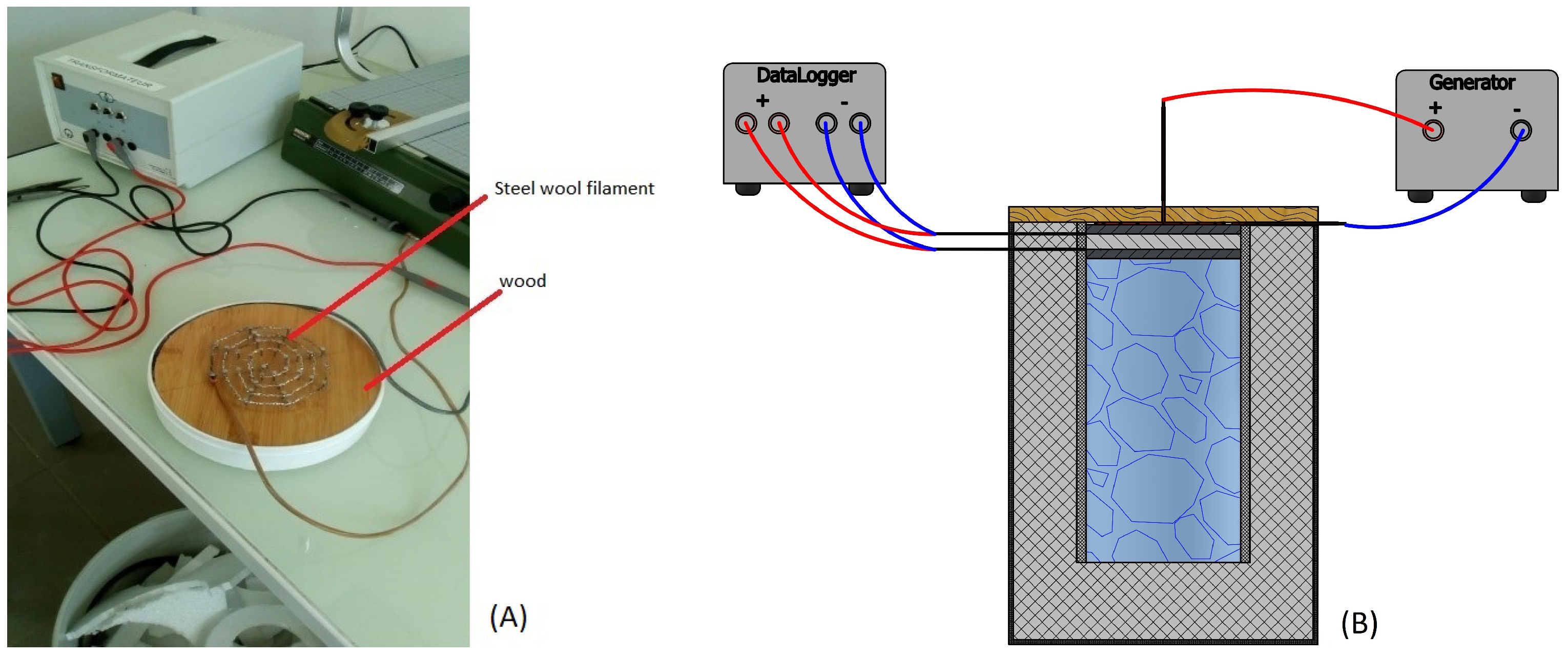
3.1. A Hot Source: Steel Wool

A piece of stainless steel wool was utilized to generate the hot heat source. The metal was wound to form a filament of specific thickness and length, as illustrated by the “hot spring” in Figure 3A. Subsequently, an electric current passes through the filament to produce heat by the Joule effect.
A variable alternating current generator (see Figure 3B) with a maximum intensity of 6 A and a maximum voltage of 10 V is connected between the two extremities of the filament. The thermal power produced by the filament is then deducted from the following formula:
P = U · I · C o s ( α )
C o s ( α ) is the power factor. There is no phase change in the active dissipative resistance of the filament. This induces α = 0 , and thus, c o s ( α ) = 1 . The dimensions of the filament are as follows: 84 cm in length and 10 cm in diameter (around nails serving as supports).

3.2. Flat Steel Iron

Flat steel irons are employed to provide support for the material testing process. This technique serves three purposes:
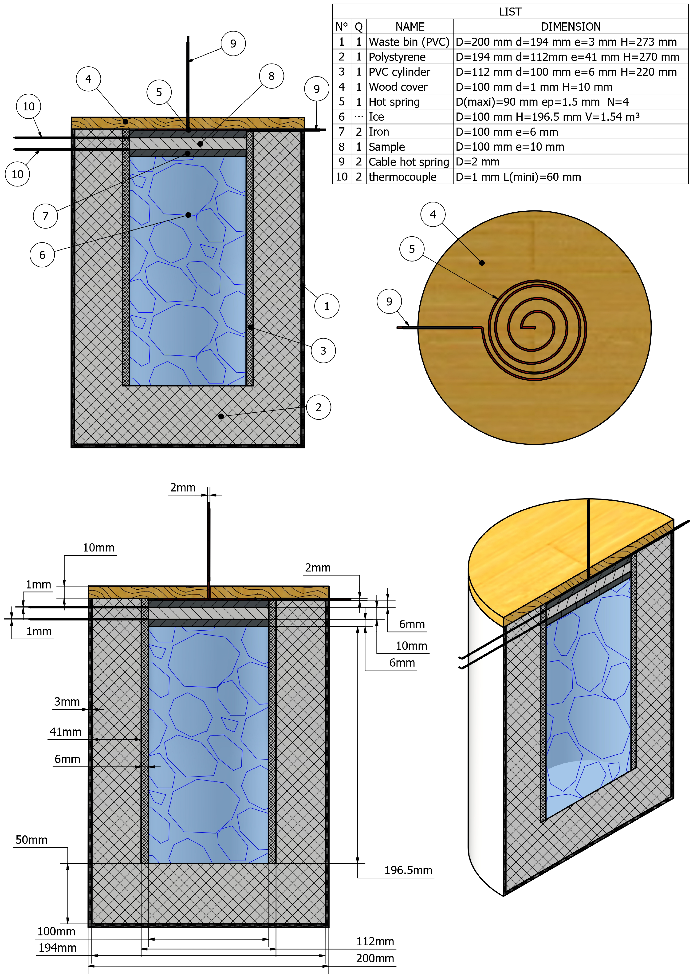
  • To ensure uniform thermal flux transfer across the entire surface of the test material. The sample diameter must match that of the flat steel iron (see Figure 2 for the dimension of the flat steel iron).
  • To accelerate the heat transfer process between the two sample surfaces in contact with the cold and hot source of the device.
  • To secure the sample from too high or too low temperatures from hot and cold heat sources of the device.

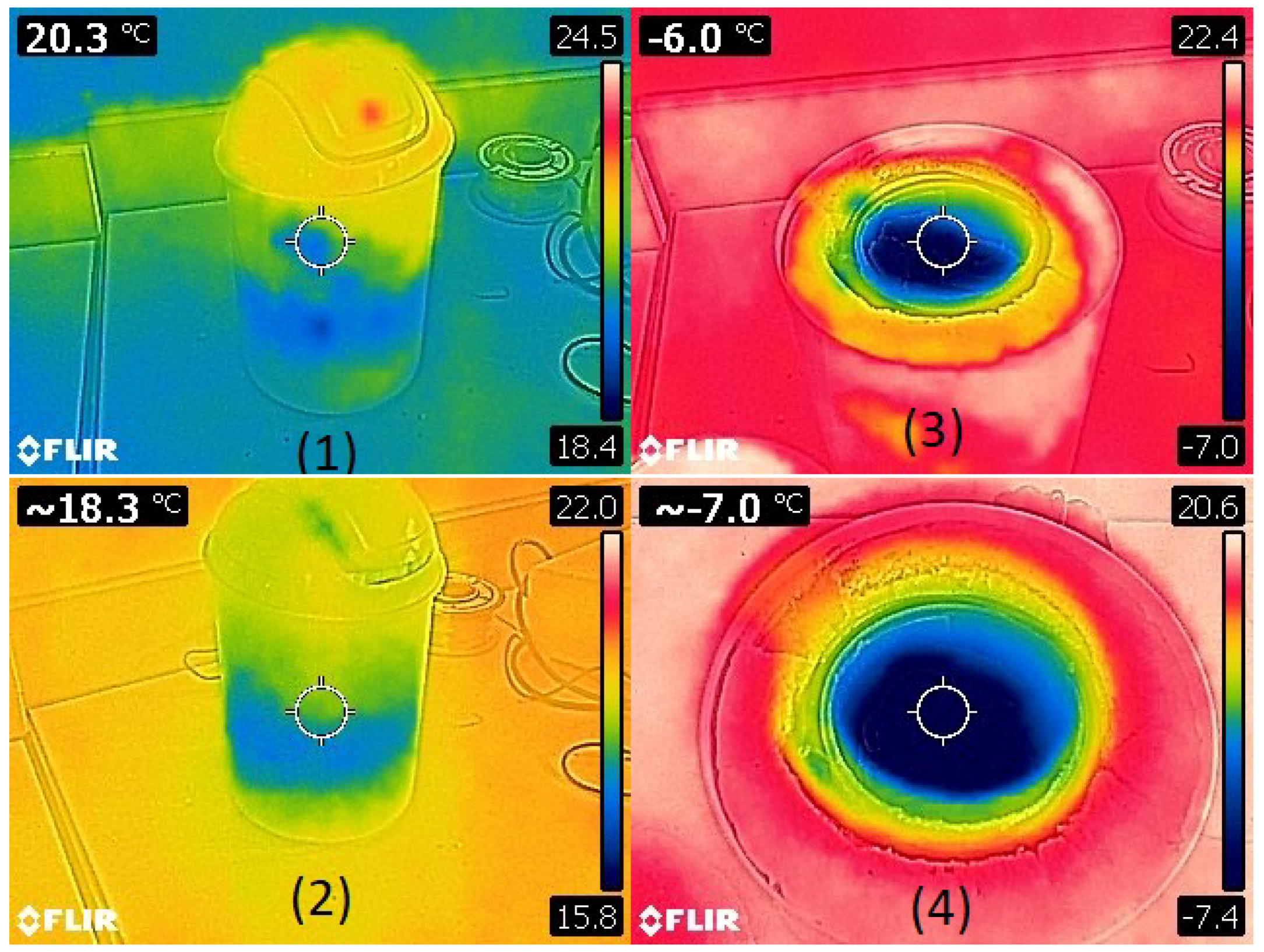
3.3. A Cold Source: The Ice Cubes

The ice cubes are hermetically isolated and represent the cold source of the device (see Figure 2). The isolation, utilized from polystyrene material, can keep the temperature of the ice cubes constant for ten hours. The ice cubes are deposited in a cylindrical compartment of 0.157 cm 3 .

3.4. The Adiabatic Part of the Device

The calorimeter is insulated with a 3.5 cm thick expanded polystyrene. The insulate is maintained by two PVC cylinders, one grey on the inside and one white on the outside, as depicted in Figure 2. The selection of materials for designing the compartment is economical and technically reliable. PVC, known for its low cost and minimal thermal conductivity ranging between 0.037 and 0.039 W · m 1 · K 1 , is an excellent supplementary insulator alongside the affordable polystyrene, which also boasts excellent insulating properties. Consequently, radial flows ( ϕ t r a n s ) can be disregarded, and only the descending flows ( ϕ d e s c ) from the heat source of our device, illustrated in Figure 4, are considered in the measurement and the thermal conductivity value calculation.

3.5. Calibration Tests and Measurement Protocol

Verification tests were conducted to assess the reliability of our cold and hot sources and measurement sensors. Subsequently, a protocol for measuring the thermal conductivity of samples utilizing the TPS technique was realized. All this work is described in this section.

3.5.1. Cold Source Verification Test

The exterior PVC is a small office waste bin measuring 18 cm in diameter, 27 cm in height, and 2 mm thick. Tests of the heat retention (cold and hot) of our sources were carried out to ensure the duration of the maintenance of the temperature of each of them in the compartment. An infrared (i.e., IR) camera enabled these tests to be carried out. The IR camera permits the observation of the qualitative aspect of heat exchange between the thermal conductivity measurement device and the external environment. The aim was to confirm the system’s overall thermal insulation, demonstrating that the device is hermetically closed over an extended period, i.e., more than 7 h of potential insulation. During the measurements of the sample, an IR camera was not used. The test protocol consisted of thermal imaging of the device containing the source (either cold or hot) and its environment over a defined period. Figure 5 shows the results obtained from the cold source test. The final result indicates that the source’s temperature varied only one degree after 7 h (i.e., 0.07 °C after 30 min. See Figure 5 for the experimentation test case). This time is much longer than the time used to measure the thermal conductivity of our sample (i.e., 15 or 30 min).
During the experiment, ice storage was performed in the thermally insulated cylinder compartment to verify that the system could sustain the heat flux from the ice cubes at 0 °C (cold source). The ice solids were retained within the enclosed adiabatic system for seven hours (refer to Figure 2). The results show that the system maintained the ice’s temperature correctly, with only 1 °C lost during the seven-hour experiment.

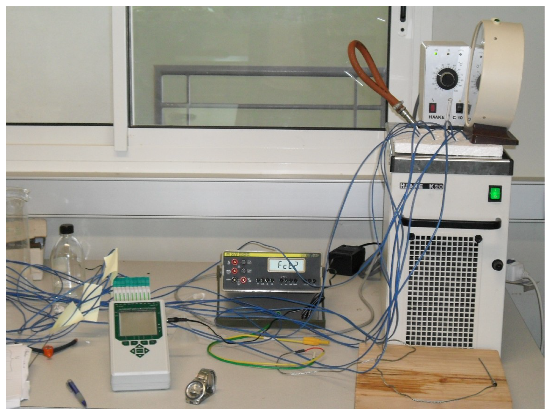
3.5.2. Hot Source Verification Test

We performed verification experiments to measure the power dissipated by Joule heating in our system and its connection to the iron plate temperature in contact with the hot source. We found a linear curve for this dissipated power as a function of temperature. The small sample size affects the heat source’s effect on the sample surface. The steel wool filament (see Figure 3A) produces heat using an AC generator with a maximal output of 33.93 watts (12.96 to 33.93 watts). The power in issue controls the heat flux through the samples.
Several tests were carried out to know the necessary power required for reaching 100 °C (a further range is not pertinent to this experiment) without the steel iron filament (see Figure 3) breaking. The experimental results are given in Table 1. The experimentation was conducted for the following three reasons:
  • To determine the optimal power level that would permit heat transfer into the tested material without causing it to catch fire;
  • To ensure that temperatures can be raised to 100 °C and to determine the precise power value necessary to achieve this temperature at the hot source; and
  • And lastly, to ensure that applying a current does not cause the iron filament to break (excessive power circulating through the filament may cause the cable to fuse). Following a series of experiments, it was determined that the ideal nominal power value is 33.9 W.
As previously stated, the impact of temperature (controlled by the electrical power of the heater) on thermal conductivity measurements was studied through a series of long-duration tests (approximately 7 h). It was found that the hot heat source varied by only 1 °C after 7 h of operation in the compartment. We therefore concluded that 15 min of measurements is more than sufficient to obtain a stable (constant) hot temperature value.

3.5.3. Thermocouple Calibrations

A LAUDA thermostat (model RE 104) was employed to calibrate the thermocouples Type T (see Figure 6) used during the experiments (refer to Appendix A for further details). The global relative error of each thermocouple does not exceed 0.90%.

3.5.4. Uncertainty of the Prototype Estimation

Multiple measurements (repeatability and accuracy) were carried out to ensure the reliability of the data. Delort et al.’s approach [40] was used to calculate experimental setup measurement uncertainty. Table 2 provides a detailed description of these global measurement uncertainties (including systematic uncertainties). The result of the overall error calculations was estimated to be approximately ±4.88%.

3.5.5. Protocol of Measurements

The sample is positioned in the intermediate space between two metallic cylinders (refer to Figure 2). The cold and hot sources, represented, respectively, by ice cubes and steel wool filament crossed by a current, are positioned opposite each other on the two metals, as illustrated in Figure 2 and Figure 3. The thermal equilibrium state (i.e., steady state) is reached after 40 min. Four thermocouples, denoted as T 0 , T 1 , T 2 , and T 3 , are positioned intermediately among the various materials (for their respective positions, refer to Figure 3). The measurements collected are taken at 1 min intervals and then averaged over 40 min. The measurements are conducted three times to ensure that the results are reliable. The measurement acquisition chain, encompassing the construction of the calorimeter, the utilization of type T thermocouples, the use of connection cables, and the data acquisition system (or datalogger) employed, conforms to the ASTM E1225 standard (i.e., the global error measurement does not exceed 5%). For more information about the error value, see the technical note of the ASTM International [41].

4. Cost of the Device

Most materials used to construct the experimental device described in this work can be recycled, and all the materials are readily available around us. If they were to be purchased, the overall financial cost of these materials would amount to approximately EUR 94.30 (see Table 3 for the specification price). Since the data acquisition unit is the most expensive device, replacing it with a multi-meter is possible. In this case, the thermocouples can be calibrated using the voltage signal that they deliver, which is read directly on the voltmeter. The cost of a voltmeter of higher accuracy is approximately EUR 94.30.

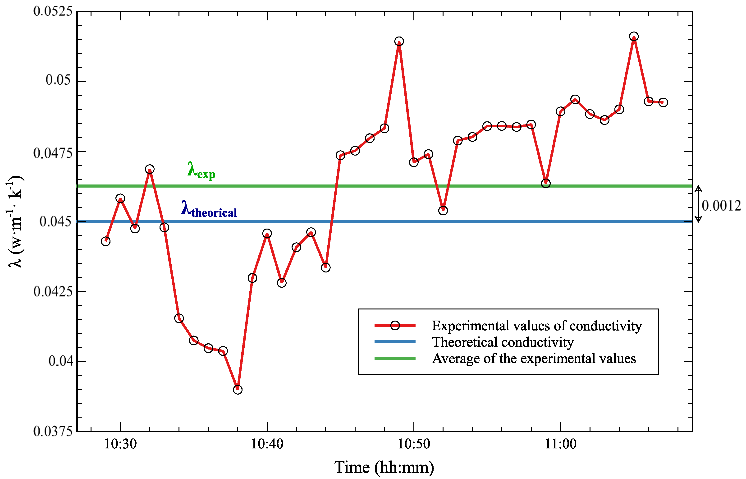
5. Results and Discussion

Three samples with known thermal conductivity (manufacturer data) were tested using the prototype designed: polystyrene, hard foam, and chipboard wood. The thermal conductivity measurement range λ WAS between 0 and 0.16 W · m 1 · K 1 , corresponding to categories of highly insulating materials. Rock wool [42], often known as mineral wool, is one example of such a material. These materials are widely utilized in buildings as thermal and acoustic insulation. Rock wool typically has a lower thermal conductivity (0.035–0.045 W · m 1 · K 1 ). Other insulating materials on the market include silica aerogel-containing building materials. Their thermal conductivity can reach 0.16 W · m 1 · K 1 (see [43] for more information). Numerous tests determined the sample size suitable for thermal conductivity experimental characterization. The sample had a diameter of 0.10 m and a thickness of 0.01 m. This work aimed to verify the reliability of the experiment device to measure the thermal conductivity of the samples. Table 4 summarizes the results obtained.
The mean thermal conductivity values collected from each sample during the experiment represent the experimental values provided by the device for each sample. By comparing the measured and reference values for the three samples, which should not exceed an acceptable error of 5%, it is reasonable to conclude that the device is functioning correctly. Figure 7 illustrates the measured values derived in the investigation of polystyrene and demonstrates how to determine the measured λ values of measurements exploit.
The measurements were taken every minute and then averaged throughout 15 to 30 min (to account for the thermal inertia of the sample) for approximately 1 h and 25 min (the experiment began precisely at 10:25 and ended around 11:10). The results obtained are depicted in Figure 7, which features a precise ordinate scale (i.e., λ values) that ranges from 0.375 to 0.525 W · m 1 · K 1 . The significant fluctuation results from the short calculation time (1 min), insufficient to observe the true evolution of λ . To reach thermal equilibrium, a 15–30 min time step is needed. Ideally, averaging these values would reduce experimental λ fluctuations influenced by Δ T variation between sample surfaces. Figure 7 illustrates calculating experimental λ values by monitoring at 1 min intervals for 1 h 25 min over a 30 min time step. Further analysis of the curve related to the material under investigation, particularly polystyrene (i.e., which exhibited the highest error during the experiment), reveals an absolute error value of approximately 0.0012 W · m 1 K 1 . These case studies (i.e., relative measurement errors observed during the experiments) confirm the consistency with the uncertainty calculation value of the new “conductometer” prototype obtained in Table 2 (i.e., not exceeding 4.88% uncertainty estimation), and give an idea of the device’s measurement accuracy. Compared to Fakra et al. [38], this study’s device can characterize construction materials with a similar error range (not exceeding 5%) as the prototype in [38] but at a lower cost. The two measuring procedures proposed in this study and [38] employ similar sample sizes. The experimental setup proposed in this work (i.e., ice production for the cold source and Joule heating for the hot source) uses less energy than the one proposed in [38], which uses Peltier plates.

6. Conclusions

Experimental research poses a significant challenge for developing countries, often due to the prohibitively high costs of acquiring the necessary measuring equipment for conducting such experiments. The field of civil engineering is no exception to this challenge. This study proposed an experimental device capable of measuring an opaque and homogeneous material’s thermal conductivity. This eco-designed and highly reliable device perfectly meets researchers’ expectations in developing countries. Indeed, it offers the following advantages: it is easy to manufacture (i.e., reproducible), very cost-effective, and user-friendly. Measurements on reference material samples were conducted to ensure the device’s reliability. The test results demonstrate that the machine can accurately determine the average values of the thermal conductivity of a construction material by ASTM E1225 Standard (see [41]). The prospects of this work would involve conducting studies to enhance the apparatus for accurately measuring thermal conductivity in non-homogeneous and non-opaque building materials, such as reflective thin products, phase change materials, translucent materials, or chromatic materials. The apparatus would also need to characterize the thermal conductivity of innovative next-generation materials already in the construction market. The thermal conductivity measurement device proposed in this paper only measures excellent insulating building materials. High-thermal-conductivity samples should be studied. Also, regarding the experimental setup proposed in this works, it is not possible to extend the measurements over time for one reason: the temperature of the cold source (the ice) tends to increase, leading to a loss of its initial volume and thereby reducing its ability to maintain the cold side of the sample wall at 0 °C after more than an hour of experimentation. Therefore, we recommend conducting experiments that do not exceed 30 min due to this limitation in the time of the cold source in the system. Another possible improvement of the test study is testing novel building materials, such as semi-transparent, translucent, and phase-change materials.

Author Contributions

Conceptualization, D.A.H.F.; methodology, D.A.H.F.; validation, D.A.H.F.; formal analysis, D.A.H.F., R.R., M.H.R., M.P.R. and R.B.; investigation, D.A.H.F.; resources, D.A.H.F.; data curation, D.A.H.F.; writing—original draft preparation, D.A.H.F.; writing—review and editing, D.A.H.F.; visualization, D.A.H.F., R.R., M.H.R., M.P.R. and R.B.; supervision, D.A.H.F.; project administration, D.A.H.F.; funding acquisition, D.A.H.F. All authors have read and agreed to the published version of the manuscript.

Funding

This research received no external funding.

Data Availability Statement

The measurement databases for this study are available upon request from the corresponding author.

Acknowledgments

The authors thank Valentin BERNOVILLE, the Scientific Instrumentation and Experimentation Technician at the University of Lorraine’s LERMAB laboratory, for designing and providing Figure 2, Figure 3B and Figure 4 of this study.

Conflicts of Interest

The authors declare no conflicts of interest.

Nomenclature

The following nomenclature is used in this manuscript:
T 0 Hot source thermocouple measurement (in K).
T 1 The thermocouple that measures the sample’s heated surface temperature (in K).
T 2 The thermocouple that measures the sample’s cooled surface temperature (in K).
T 3 Cold source thermocouple measurement (in K).
T i Surface temperature of any material (in K).
ϕ Constant thermal flux crossing an opaque wall (in W).
ϕ d e s c 
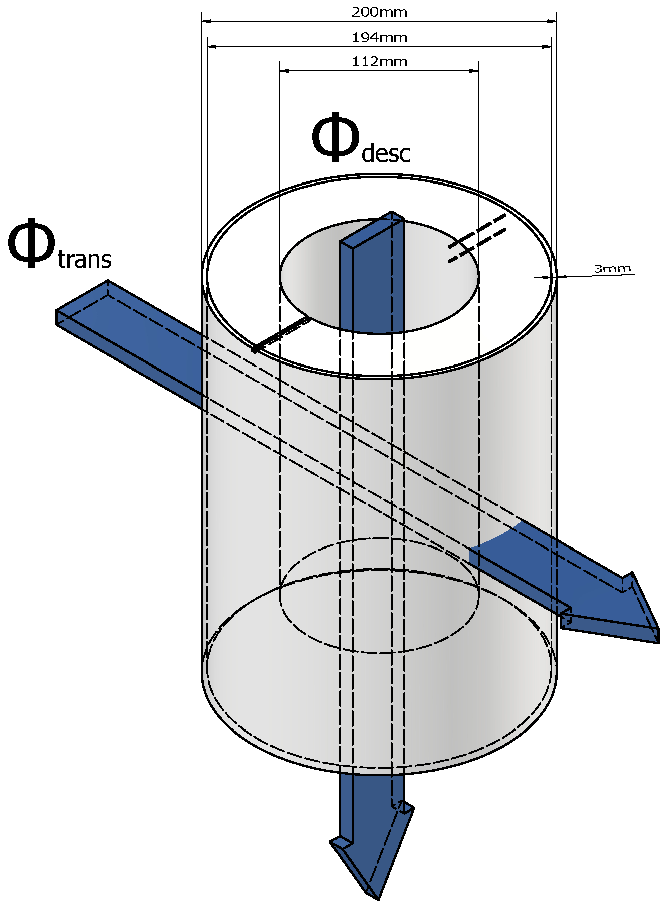
Downward thermal flux through the experimental setup (in W).
ϕ t r a n s Thermal flux passing horizontally through the experimental setup (in W).
eThickness of any material described in Table 2 (in m).
diadiameter of any material described in Table 2 (in m).
A 0 Surface of the plate steel iron (in m 2 ).
A x Surface of the sample study (in m 2 ).
d 0 Thickness of the plate steel iron (in m).
d x Thickness of the sample study (in m).
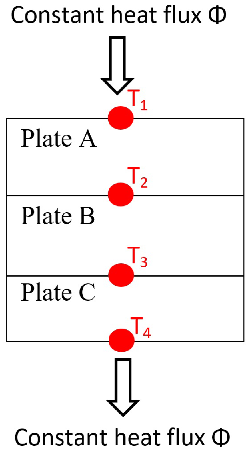
Plate ATop plate steel iron (-).
Plate Bthe sample plate study (-).
Plate CBottom plate steel iron (-).
ASTMAmerican Society for Testing and Materials.
TPSTransient plane source measurement method.
HFM“Hot flow meter” method for measuring the thermal conductivity of a material (-).
GHF“Guarded heat flow” method for measuring the thermal conductivity of a
material (-).
GHP“Guarded hot plate” method for measuring the thermal conductivity of a
material (-).
GHB“Guarded hot box” method for measuring the thermal conductivity of a material (-).
IRT“Infrared thermography” method for measuring the thermal conductivity of a
material (-).
SHB“Surface heat balance” method for measuring the thermal conductivity of a
material (-).
TBM“Temperature-based method” for measuring the thermal conductivity of a
material (-).
TCB“Transient-cylinder bridge” method for measuring the thermal conductivity of a
material (-).
PPower delivered by the generator (in W).
UVoltage delivered by the generator (in V).
IIntensity delivered by the generator (in A).
α Phase angle between current and voltage (in °).
λ e x p Thermal conductivity of the experimental sample measured in the device
(in W · m 1 · K 1 ).
λ t h e o r e t i c a l Thermal conductivity reference of the sample given by the manufacturer
(in W · m 1 · K 1 ).

Appendix A

Table A1. Specifications thermostat RE104.
RE104
Operating temperature range°C−10 to 120
Ambient temperature range°C5 …40
Setting resolution°C0.1
Indication resolution°C0.1
Heater power 230 V; 50/60 Hzkw1.5
Heater power 115 V; 60 Hz1.3
Heater power 100 V; 50/60 Hz1.0
Pump type pressure pump with choice of 5 output steps
Max. discharge pressurebar0.4
Max. flow rateL/mm17
Pump Connectionsmmnipples 13 mm dia.
Max. bath volumeL3 to 4.5
Bath opening (W × D)mm130 × 105
Bath depthmm160
Usable depthmm140
Height top edge of bathmm363
Overall size (W × D × H)mm180 × 320 × 254
Weightkg21
Power consumption 230 V; 50/60 HzKW1.7
Power consumption 115 V; 60 Hz1.4
Power consumption 100 V; 50/60 Hz1.1
Safety features FL
Temperature Control±°C0.05

Appendix B

Table A2. Specifications datalogger CR3000.
Specifications CR3000
-NOTE-Note: Additional specifications are listed in the CR3000 Specifications Sheet.
Operating Temperature Range−25 °C to +50 °C (standard) −40 °C to +85 °C (extended)Non-condensing environment
The rechargeable base option has an operating temperature range of −40 °C to +60 °C.
The alkaline base option has a temperature range of −25 °C to +50 °C.
25 °C to +50 °C (standard) −40°C to +85 °C (extended)
Analog Inputs28 single-ended or 14 differential (individually configured)
Pulse Counters4
Voltage Excitation Terminals4 (VX1 to VX4)
Communications PortsCS I/O
RS-232
Parallel peripheral
Switched 12 Volt2 terminals
Digital I/OCertain digital ports can be used to count switch closures.
3 SDM and 8 I/Os or 4 RS-232 COM I/O
Input Limits±5 Vdc
Analog Voltage Accuracy±(0.04% of reading + offset) at 0 °C to 40 °C
ADC16-bit
Power Requirements10 to 16 Vdc
Real-Time Clock Accuracy±3 min. per year (Correction via GPS optional.)
Internet ProtocolsFTP, HTTP, XML POP3, SMTP, Telnet, NTCIP, NTP,
Communication ProtocolsPakBus, Modbus, DNP3, SDI-12, SDM
Warranty3 years
Idle Current Drain, Average2 mA (@ 12 Vdc)
Active Current Drain, Average3 mA (1 Hz sample rate @ 12 Vdc without RS-232 communication)
10 mA (100 Hz sample rate @ 12 Vdc without RS-232 communication)
38 mA (100 Hz sample rate @ 12 Vdc with RS-232 communication)

References

  1. Asadi, I.; Shafigh, P.; Hassan, Z.F.B.A.; Mahyuddin, N.B. Thermal conductivity of concrete—A review. J. Build. Eng. 2018, 20, 81–93. [Google Scholar] [CrossRef]
  2. Yüksel, N. The Review of Some Commonly Used Methods and Techniques to Measure the Thermal Conductivity of Insulation Materials. In Insulation Materials in Context of Sustainability; IntechOpen: London, UK, 2016. [Google Scholar] [CrossRef]
  3. Gomes, M.G.; Flores-Colen, I.; Da Silva, F.; Pedroso, M. Thermal conductivity measurement of thermal insulating mortars with EPS and silica aerogel by steady-state and transient methods. Constr. Build. Mater. 2018, 172, 696–705. [Google Scholar] [CrossRef]
  4. Boudenne, A.; Ibos, L.; Gehin, E.; Candau, Y. A simultaneous characterization of thermal conductivity and diffusivity of polymer materials by a periodic method. J. Phys. D Appl. Phys. 2003, 37, 132. [Google Scholar] [CrossRef]
  5. Hu, R.; Ma, A.; Li, Y. Transient hot strip measures thermal conductivity of organic foam thermal insulation materials. Exp. Therm. Fluid Sci. 2018, 91, 443–450. [Google Scholar] [CrossRef]
  6. Cesaratto, P.G.; De Carli, M. A measuring campaign of thermal conductance in situ and possible impacts on net energy demand in buildings. Energy Build. 2013, 59, 29–36. [Google Scholar] [CrossRef]
  7. Cuce, E.; Cuce, P.M.; Guclu, T.; Besir, A.; Gokce, E.; Serencam, U. A novel method based on thermal conductivity for material identification in scrap industry: An experimental validation. Measurement 2018, 127, 379–389. [Google Scholar] [CrossRef]
  8. Kim, K.H.; Jeon, S.E.; Kim, J.K.; Yang, S. An experimental study on thermal conductivity of concrete. Cem. Concr. Res. 2003, 33, 363–371. [Google Scholar] [CrossRef]
  9. Guo, L.; Guo, L.; Zhong, L.; Zhu, Y. Thermal conductivity and heat transfer coefficient of concrete. J. Wuhan Univ. Technol.-Mater. Sci. Ed. 2011, 26, 791–796. [Google Scholar] [CrossRef]
  10. Desogus, G.; Mura, S.; Ricciu, R. Comparing different approaches to in situ measurement of building components thermal resistance. Energy Build. 2011, 43, 2613–2620. [Google Scholar] [CrossRef]
  11. Ahmad, A.; Maslehuddin, M.; Al-Hadhrami, L.M. In situ measurement of thermal transmittance and thermal resistance of hollow reinforced precast concrete walls. Energy Build. 2014, 84, 132–141. [Google Scholar] [CrossRef]
  12. Cesaratto, P.G.; De Carli, M.; Marinetti, S. Effect of different parameters on the in situ thermal conductance evaluation. Energy Build. 2011, 43, 1792–1801. [Google Scholar] [CrossRef]
  13. Asdrubali, F.; Baldinelli, G. Thermal transmittance measurements with the hot box method: Calibration, experimental procedures, and uncertainty analyses of three different approaches. Energy Build. 2011, 43, 1618–1626. [Google Scholar] [CrossRef]
  14. Zhu, X.; Li, L.; Yin, X.; Zhang, S.; Wang, Y.; Liu, W.; Zheng, L. An in-situ test apparatus of heat transfer coefficient for building envelope. Build. Energy Effic. 2012, 256, 57–60. [Google Scholar]
  15. Albatici, R.; Tonelli, A.M.; Chiogna, M. A comprehensive experimental approach for the validation of quantitative infrared thermography in the evaluation of building thermal transmittance. Appl. Energy 2015, 141, 218–228. [Google Scholar] [CrossRef]
  16. Fokaides, P.A.; Kalogirou, S.A. Application of infrared thermography for the determination of the overall heat transfer coefficient (U-Value) in building envelopes. Appl. Energy 2011, 88, 4358–4365. [Google Scholar] [CrossRef]
  17. Barreira, E.; Almeida, R.; Delgado, J. Infrared thermography for assessing moisture related phenomena in building components. Constr. Build. Mater. 2016, 110, 251–269. [Google Scholar] [CrossRef]
  18. Evangelisti, L.; Guattari, C.; Gori, P.; De Lieto Vollaro, R. In situ thermal transmittance measurements for investigating differences between wall models and actual building performance. Sustainability 2015, 7, 10388–10398. [Google Scholar] [CrossRef]
  19. Nardi, I.; Ambrosini, D.; de Rubeis, T.; Sfarra, S.; Perilli, S.; Pasqualoni, G. A comparison between thermographic and flow-meter methods for the evaluation of thermal transmittance of different wall constructions. J. Phys. Conf. Ser. 2015, 655, 012007. [Google Scholar] [CrossRef]
  20. Nardi, I.; Paoletti, D.; Ambrosini, D.; De Rubeis, T.; Sfarra, S. U-value assessment by infrared thermography: A comparison of different calculation methods in a Guarded Hot Box. Energy Build. 2016, 122, 211–221. [Google Scholar] [CrossRef]
  21. Glavaš, H.; Hadzima-Nyarko, M.; Haničar Buljan, I.; Barić, T. Locating hidden elements in walls of cultural heritage buildings by using infrared thermography. Buildings 2019, 9, 32. [Google Scholar] [CrossRef]
  22. Evangelisti, L.; Scorza, A.; De Lieto Vollaro, R.; Sciuto, S.A. Comparison between heat flow meter (HFM) and thermometric (THM) method for building wall thermal characterization: Latest advances and critical review. Sustainability 2022, 14, 693. [Google Scholar] [CrossRef]
  23. Rausch, M.H.; Krzeminski, K.; Leipertz, A.; Fröba, A.P. A new guarded parallel-plate instrument for the measurement of the thermal conductivity of fluids and solids. Int. J. Heat Mass Transf. 2013, 58, 610–618. [Google Scholar] [CrossRef]
  24. Chen, F.; Wittkopf, S.K. Summer condition thermal transmittance measurement of fenestration systems using calorimetric hot box. Energy Build. 2012, 53, 47–56. [Google Scholar] [CrossRef]
  25. Meng, X.; Gao, Y.; Wang, Y.; Yan, B.; Zhang, W.; Long, E. Feasibility experiment on the simple hot box-heat flow meter method and the optimization based on simulation reproduction. Appl. Therm. Eng. 2015, 83, 48–56. [Google Scholar] [CrossRef]
  26. Meng, X.; Luo, T.; Gao, Y.; Zhang, L.; Shen, Q.; Long, E. A new simple method to measure wall thermal transmittance in situ and its adaptability analysis. Appl. Therm. Eng. 2017, 122, 747–757. [Google Scholar] [CrossRef]
  27. Osaze, O.; Khanna, S. Experimental Thermal Conductivity Measurement of Hollow-Structured Polypropylene Material by DTC-25 and Hot Box Test. Buildings 2023, 13, 3094. [Google Scholar] [CrossRef]
  28. Kurpińska, M.; Karwacki, J.; Maurin, A.; Kin, M. Measurements of thermal conductivity of LWC cement composites using simplified laboratory scale method. Materials 2021, 14, 1351. [Google Scholar] [CrossRef]
  29. Mobaraki, B.; Komarizadehasl, S.; Castilla Pascual, F.J.; Lozano-Galant, J.A.; Porras Soriano, R. A novel data acquisition system for obtaining thermal parameters of building envelopes. Buildings 2022, 12, 670. [Google Scholar] [CrossRef]
  30. Vučićević, B.; Turanjanin, V.; Bakić, V.; Jovanović, M.; Stevanović, Ž. Experimental and numerical modeling of thermal performance of a residential building in belgrade. Therm. Sci. 2009, 13, 245–252. [Google Scholar] [CrossRef]
  31. Andargie, M.S.; Azar, E. An applied framework to evaluate the impact of indoor office environmental factors on occupants’ comfort and working conditions. Sustain. Cities Soc. 2019, 46, 101447. [Google Scholar] [CrossRef]
  32. Evangelisti, L.; Guattari, C.; Gori, P.; de Lieto Vollaro, R.; Asdrubali, F. Experimental investigation of the influence of convective and radiative heat transfers on thermal transmittance measurements. Int. Commun. Heat Mass Transf. 2016, 78, 214–223. [Google Scholar] [CrossRef]
  33. Ricklefs, A.; Thiele, A.M.; Falzone, G.; Sant, G.; Pilon, L. Thermal conductivity of cementitious composites containing microencapsulated phase change materials. Int. J. Heat Mass Transf. 2017, 104, 71–82. [Google Scholar] [CrossRef]
  34. Lucchi, E.; Roberti, F.; Alexandra, T. Definition of an experimental procedure with the hot box method for the thermal performance evaluation of inhomogeneous walls. Energy Build. 2018, 179, 99–111. [Google Scholar] [CrossRef]
  35. Gagliano, A.; Cascone, S. Eco-friendly green roof solutions: Investigating volcanic ash as a viable alternative to traditional substrates. Constr. Build. Mater. 2024, 411, 134442. [Google Scholar] [CrossRef]
  36. Platzer, N. Encyclopedia of Polymer Science and Engineering, H. F. Mark, N. M. Bikales, C. G. Overberger, and G. Menges, Wiley-Interscience, New York, 1985, 720 pp. J. Polym. Sci. Part C Polym. Lett. 1986, 24, 359–360. [Google Scholar] [CrossRef]
  37. Mottram, T. Thermal transport properties. Int. Encycl. Compos. 1989, 127, 379–389. [Google Scholar]
  38. Fakra, D.A.H.; José, B.R.A.; Murad, N.M.; Gatina, J.C. A new affordable and quick experimental device for measuring the thermo-optical properties of translucent construction materials. J. Build. Eng. 2020, 32, 101708. [Google Scholar] [CrossRef]
  39. Fakra, D.A.H.; José, B.R.A.; Murad, N.M.; Randriantsoa, A.N.A.; Gatina, J.C. Experimental data and calibration processes to a new and simple device dedicated to the thermo-optical properties of a polycarbonate construction material. Data Brief 2020, 32, 106289. [Google Scholar] [CrossRef]
  40. Delort, M.; Fakra, D.; Malet-Damour, B.; Gatina, J.C. Measuring the uncertainty assessment of an experimental device used to determine the thermo-optico-physical properties of translucent construction materials. Meas. Sci. Technol. 2022, 33, 055007. [Google Scholar] [CrossRef]
  41. ASTM E1225-13; Standard Test Method for Thermal Conductivity of Solids by Means of the Guarded-Comparative-Longitudinal Heat Flow Technique; Technical Report. American Society for Testing and Materials: West Conshohocken, PA, USA, 2013; 8p.
  42. Hetimy, S.; Megahed, N.; Eleinen, O.A.; Elgheznawy, D. Exploring the potential of sheep wool as an eco-friendly insulation material: A comprehensive review and analytical ranking. Sustain. Mater. Technol. 2023, 39, e00812. [Google Scholar] [CrossRef]
  43. Lamy-Mendes, A.; Pontinha, A.D.R.; Alves, P.; Santos, P.; Durães, L. Progress in silica aerogel-containing materials for buildings’ thermal insulation. Constr. Build. Mater. 2021, 286, 122815. [Google Scholar] [CrossRef]
Figure 1. Schematic view of the experimental thermal exchange model ( T 1 > T 2 > T 3 > T 4 ).
Metrology 04 00026 g001
Figure 2. Description of the conduct-meter prototype with the dimension of each component.
Metrology 04 00026 g002
Figure 3. (A): hot source of the device made with a steel wool filament and current generator; (B): data acquisition and electric current connection for respectively the thermocouple and the hot source (i.e., “hot spring”).
Metrology 04 00026 g003
Figure 4. Visualization and dimensions of calorimeter thermal insulation.
Metrology 04 00026 g004
Figure 5. Temperature observed from the infrared camera of the conduct-meter prototype outside (i.e., two pictures: (1,2)) and inside (i.e., two pictures: (3,4)) taken over seven hours. The two top images (i.e., (1,3)) indicate the initial times, and the two bottom images (i.e., (2,4)) indicate the final times.
Metrology 04 00026 g005
Figure 6. Acquisition chain (see Appendix B for more information about the datalogger CR3000) of the thermocouple Type T test calibration.
Metrology 04 00026 g006
Figure 7. Comparison of the average experimental thermal conductivity value λ e x p of the polystyrene sample with the reference value (i.e., theoretical) λ t h e o r e t i c a l (given by the manufacturer).
Metrology 04 00026 g007
Table 1. Power values obtained in the test of the hot source.
The Results of the Test (Maximum Power)
Intensities (A)Voltages (V)Temperature (K)Temperature (°C)Power (W)
162.16335.156212.96
27.773364.159123.31
38.73.9373.1510033.93
Table 2. Uncertainty of the new conductometer prototype presented in this work, inspired by the Delort et al. method [40].
The PrototypeNatureUncertainty (%)
SampleSize0.138
Positioning0.12
ThermocoupleMeasurement0.4
Data loggerData acquisition0.1
Thermal source (hot)Hot spring1.46
Thermal source (cold)Ice1.46
Conductivity lawFourier law0.079
Ironsize0.132
Positioning0.18
WiringSignal transmission0.53
IsolationSizing (PVC + polystyrene)0.2
Positioning (PVC + polystyrene)0.09
Total uncertainty4.88
Table 3. Manufacturing price of the device (estimation price on Reunion Island for the year 2021–2022).
NDesignationQDimensionsUnit Cost (EUR)Total Cost (EUR)
e (m)dia (m)
1Generator1 6363
2Steel wool1 0.500.50
3Thermocouple40.0180.14.2016.80
4Black flat steel iron20.0060.100
5Polystyrene (sample)10.010.100
6Small waste bin10.20.122
7Ice1 00
8Recycled polystyrene (isolation)1 00
9Tube PVC10.0020.111
10Plug PVC10.020.181111
Total94.30 €
Table 4. Experimental (measurement) vs. theoretical (reference) thermal conductivity values.
Type of Material λ theoretical ( W · m 1 · K 1 ) λ exp ( W · m 1 · K 1 ) Relative Error
Hard foam0.160.1553.13%
Polystyrene0.0450.04684%
Chipboard wood0.120.1172.5%
Disclaimer/Publisher’s Note: The statements, opinions and data contained in all publications are solely those of the individual author(s) and contributor(s) and not of MDPI and/or the editor(s). MDPI and/or the editor(s) disclaim responsibility for any injury to people or property resulting from any ideas, methods, instructions or products referred to in the content.

