

Geometric Calibration of Thermal Infrared Cameras: A Comparative Analysis for Photogrammetric Data Fusion

 ,
,  ,
,  , ,
, ,
Abstract
1. Introduction
1.1. Research Aims
- 1.
- Compare 2D board and 3D field calibration processes, detailing production, observation, and calculation of IO and RO parameters using three commercial software packages: MathWorks’ MATLAB, Agisoft Metashape, and Photometrix’s Australis;
- 2.
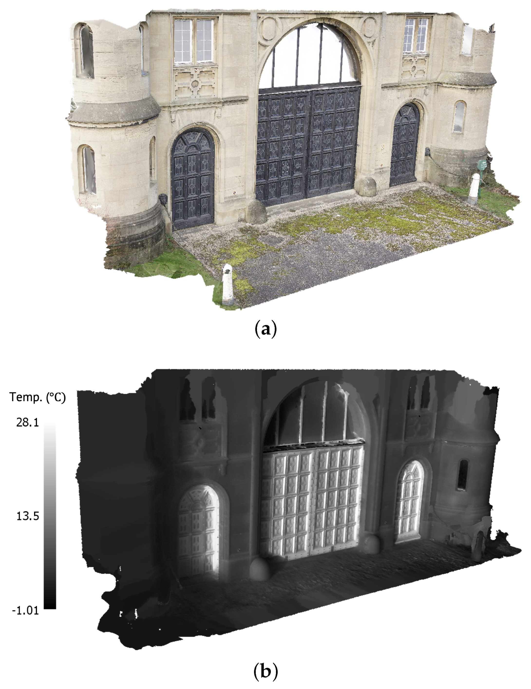
- Assess the accuracy of derived IO parameters applied to IRT-3DDF using a combined TIR-RGB bundle block adjustment for a historic building façade (Method 1);
- 3.
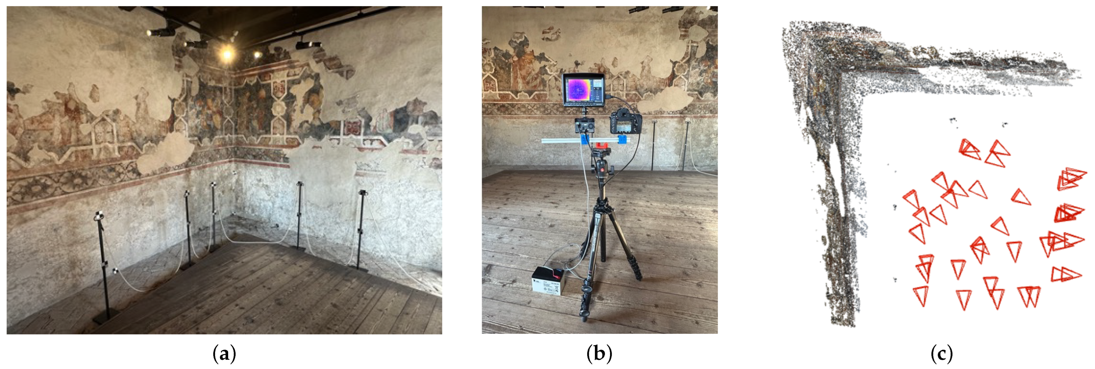
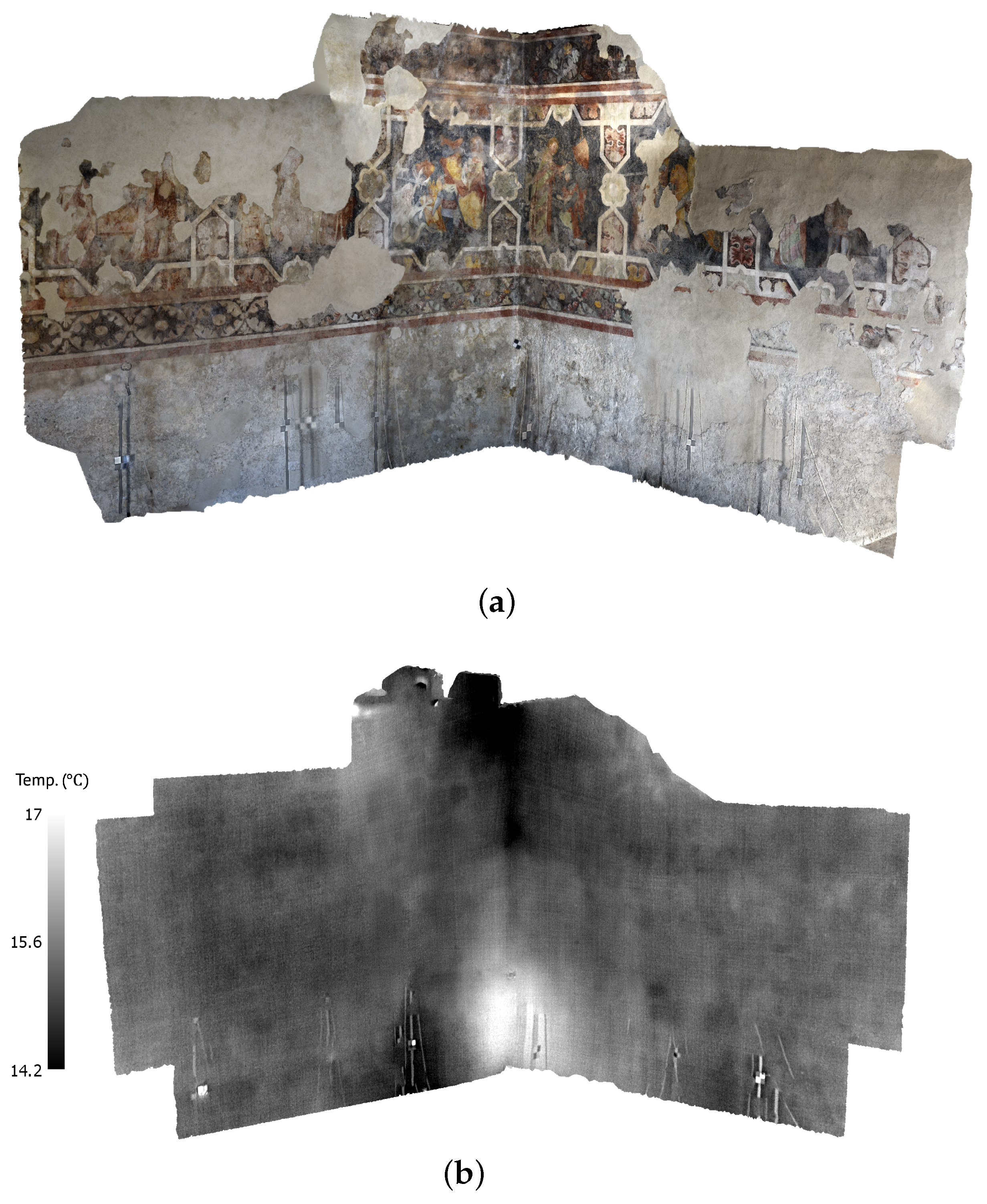
- Assess the accuracy of derived RO parameters applied to IRT-3DDF using a relative pose implementation on medieval frescoes (Method 2).
1.2. Paper Structure
2. Geometric Calibration
2.1. Cameras
2.2. Calibration Targets
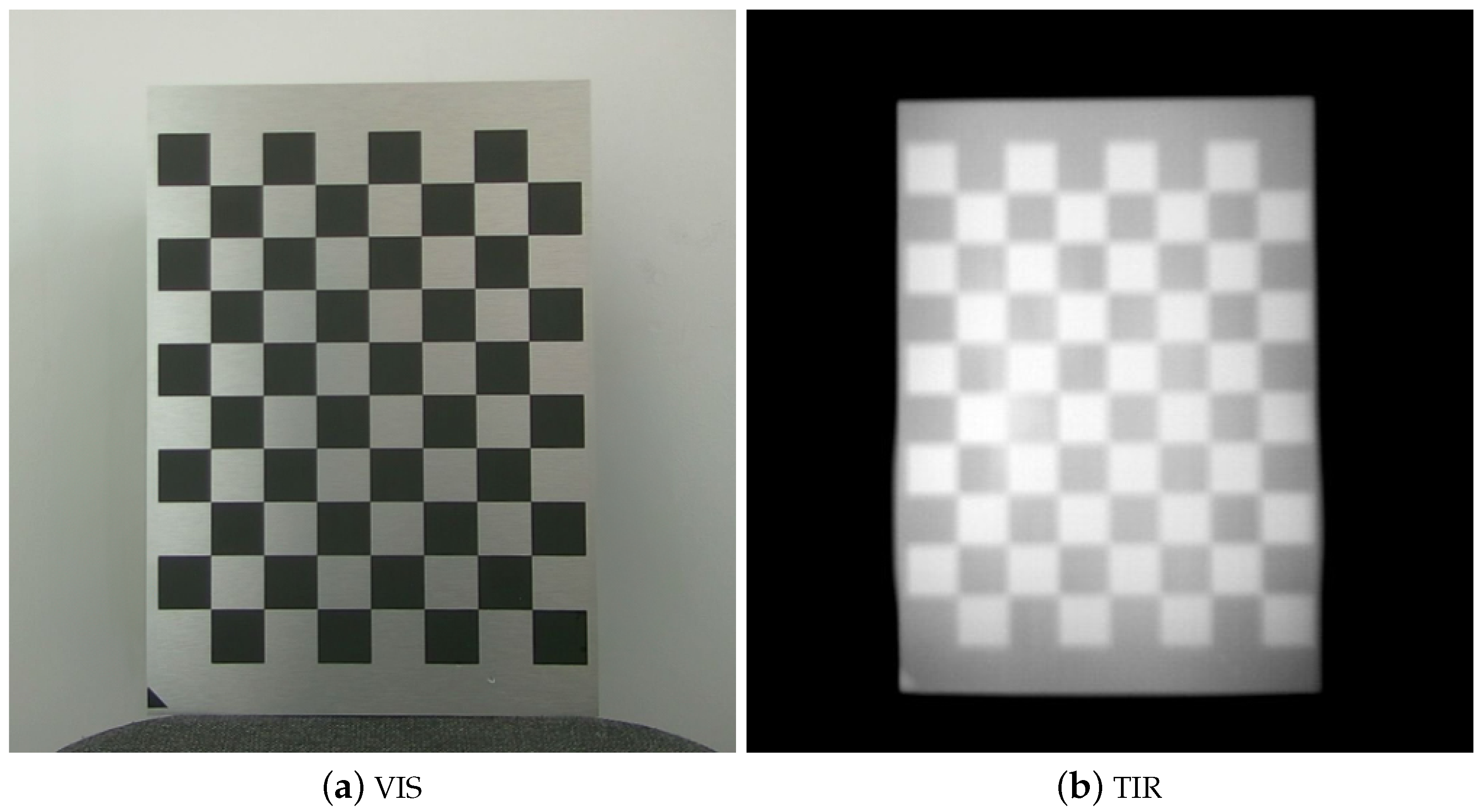
2.2.1. 2D Board
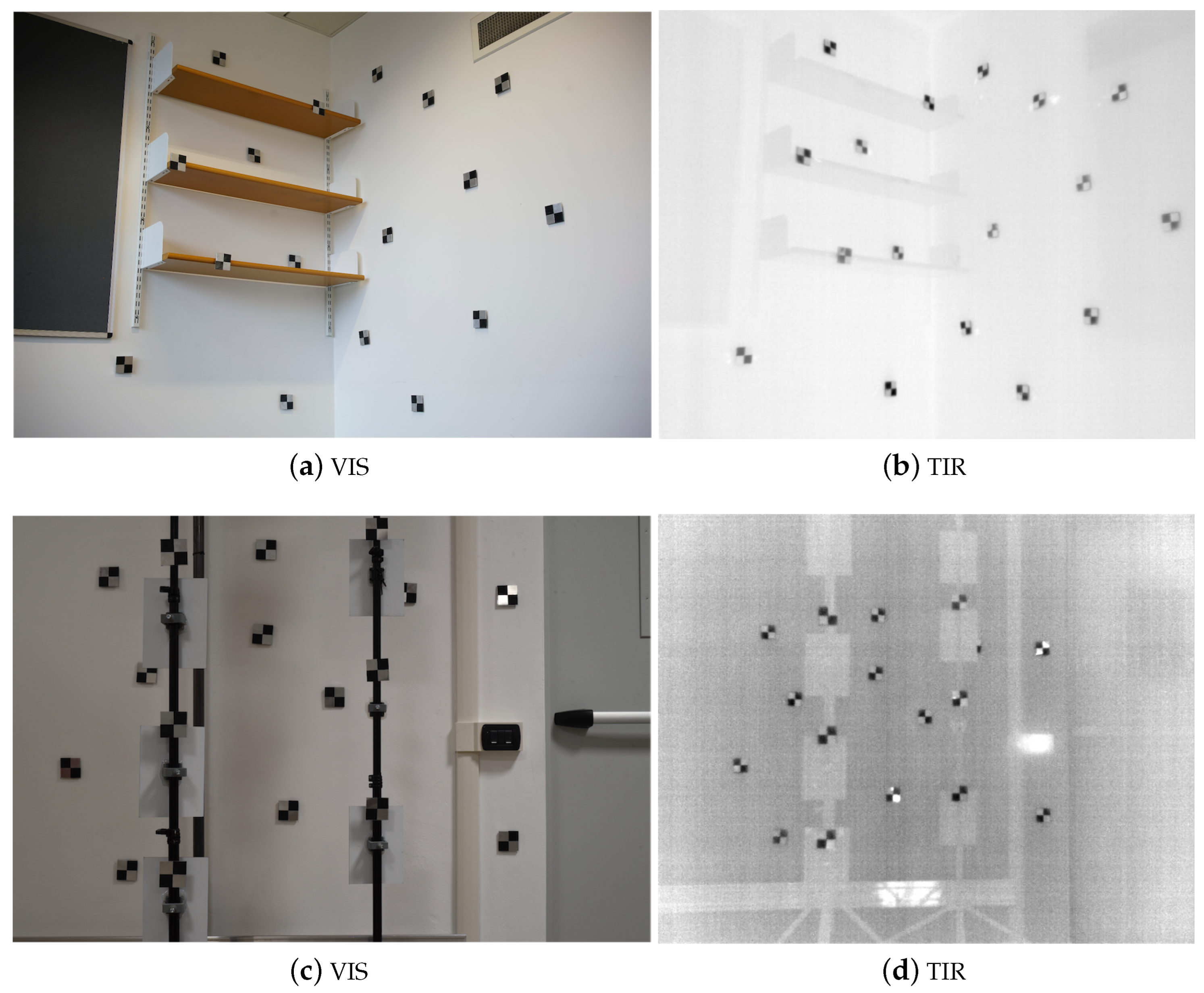
2.2.2. 3D Field
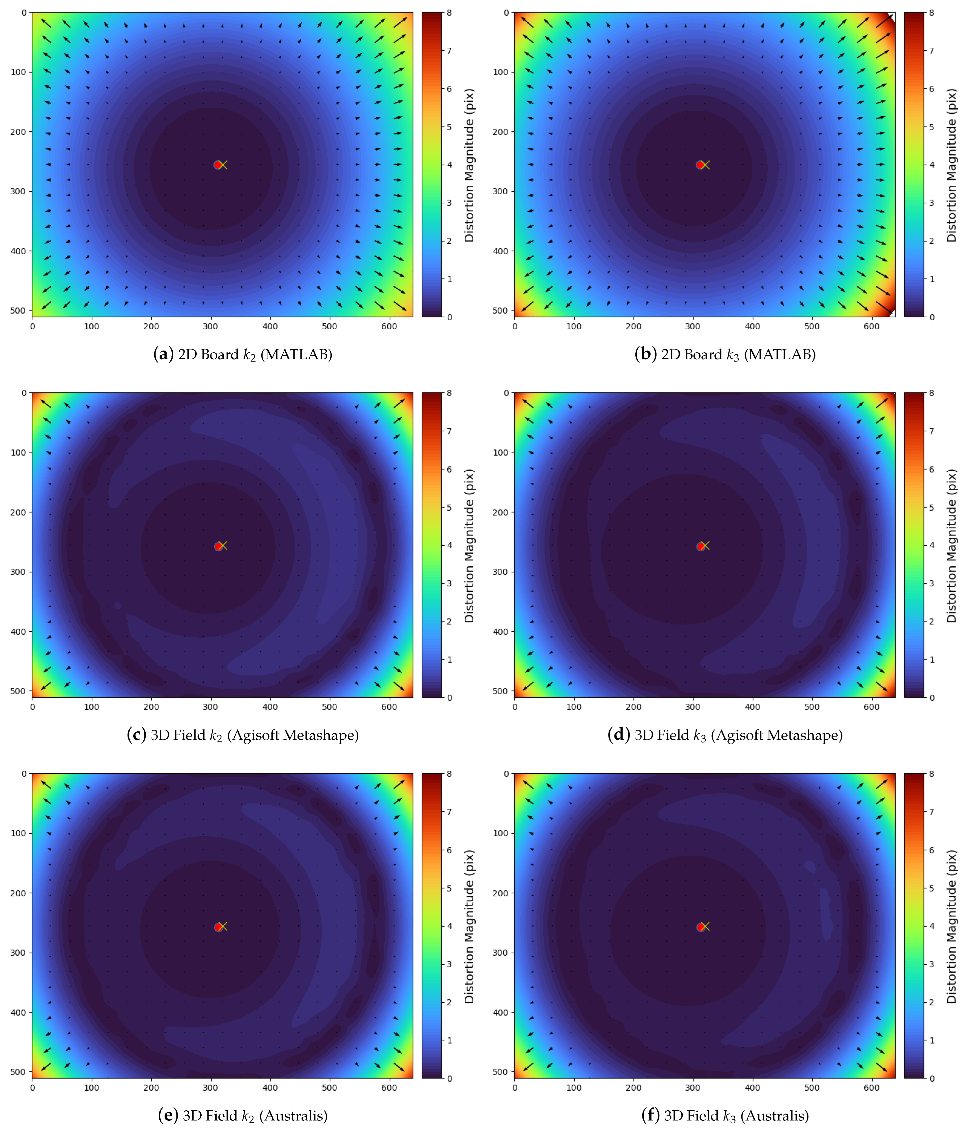
2.3. Interior Orientation
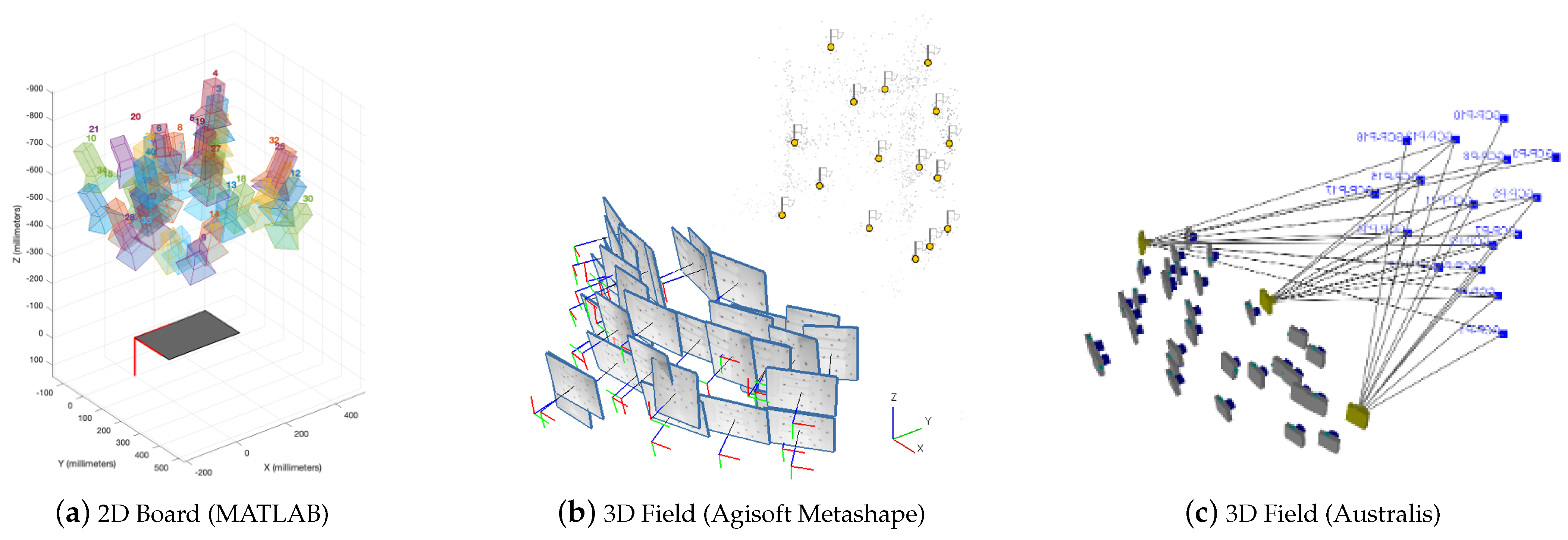
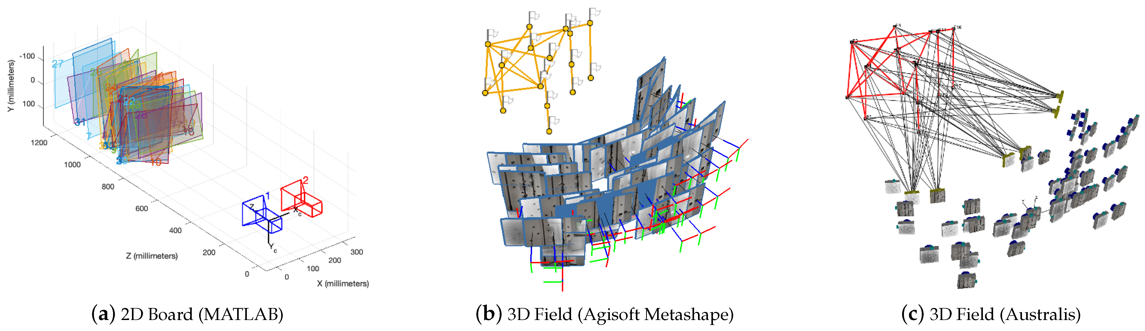
2.3.1. 2D Board (MATLAB)
2.3.2. 3D Field (Agisoft Metashape)
2.3.3. 3D Field (Australis)
2.4. Relative Orientation
2.4.1. 2D Board (MATLAB)
2.4.2. 3D Field (Agisoft Metashape)
2.4.3. 3D Field (Australis)
3. InfraRed Thermography 3D Data Fusion (IRT-3DDF)
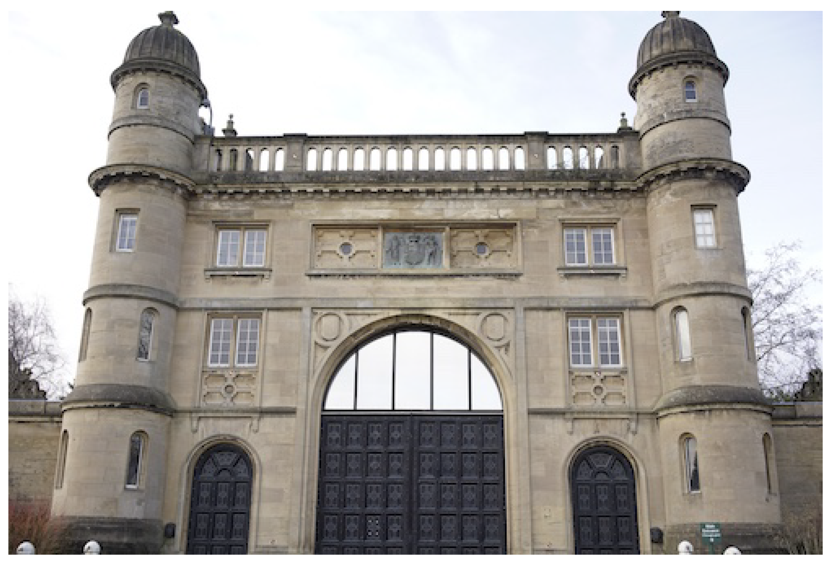
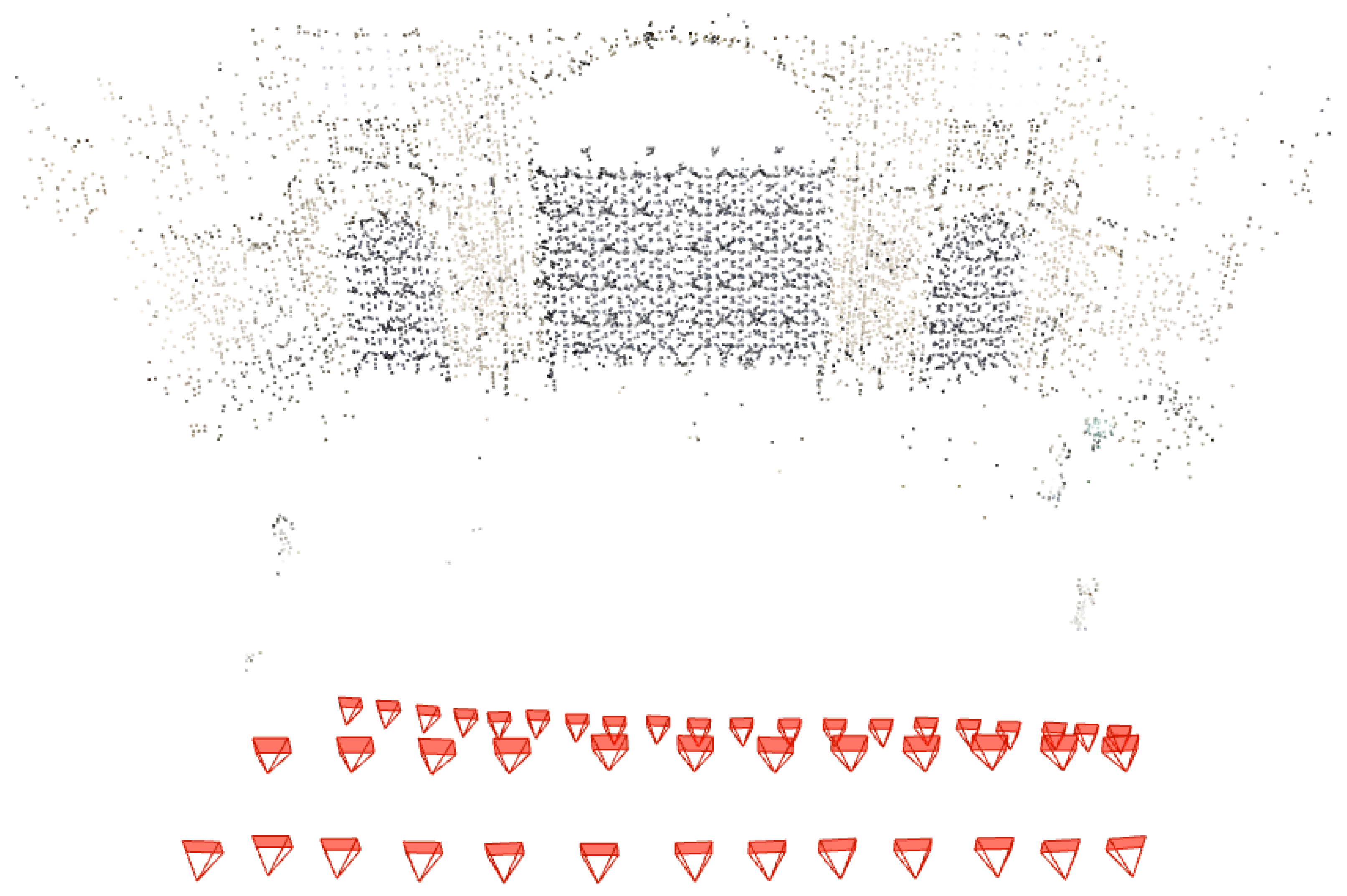
3.1. Method 1: Combined TIR-RGB Bundle Block Adjustment
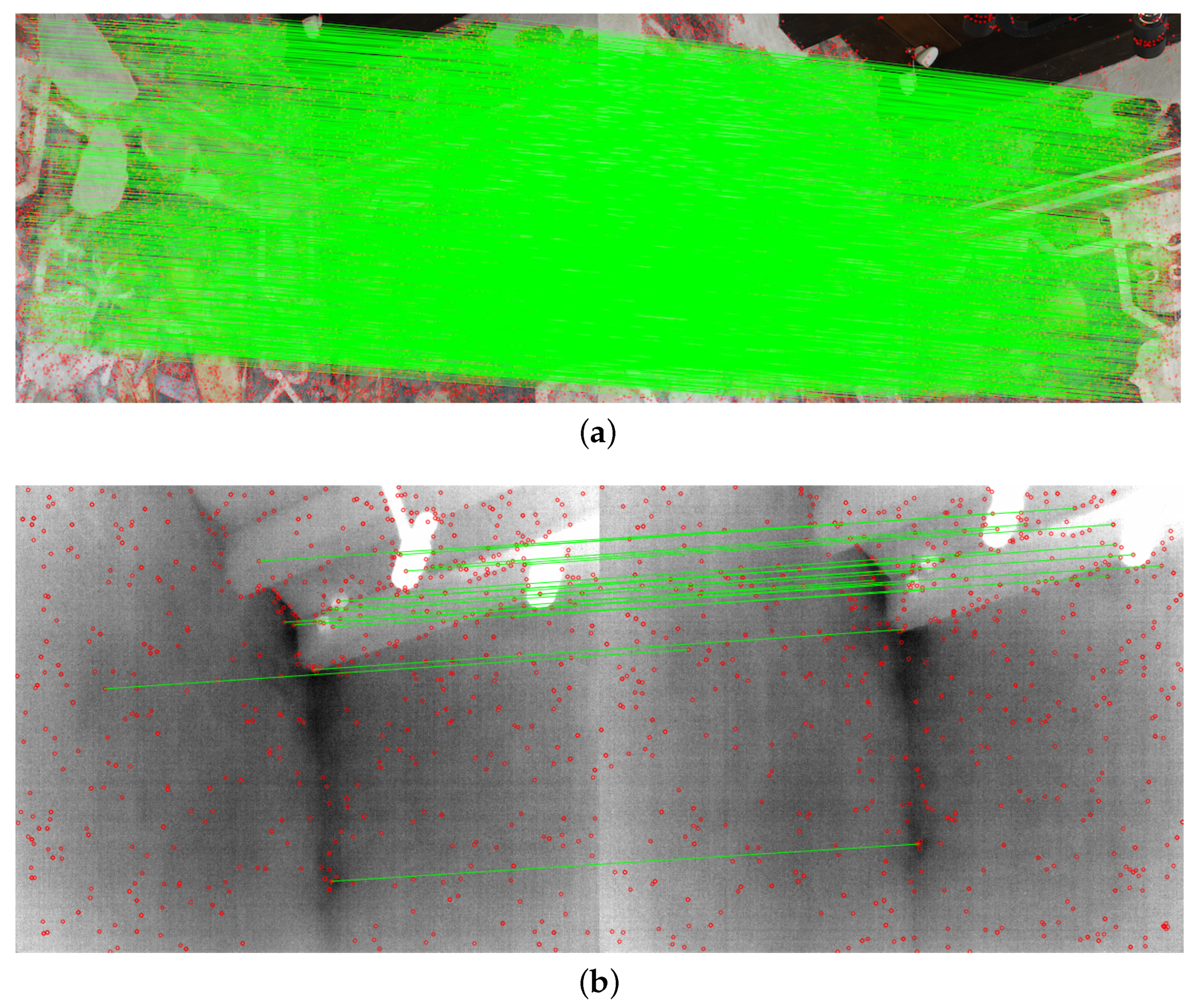
3.2. Method 2: Relative Pose Implementation
4. Discussion
4.1. TIR Geometric Calibration
4.1.1. Calibration Targets
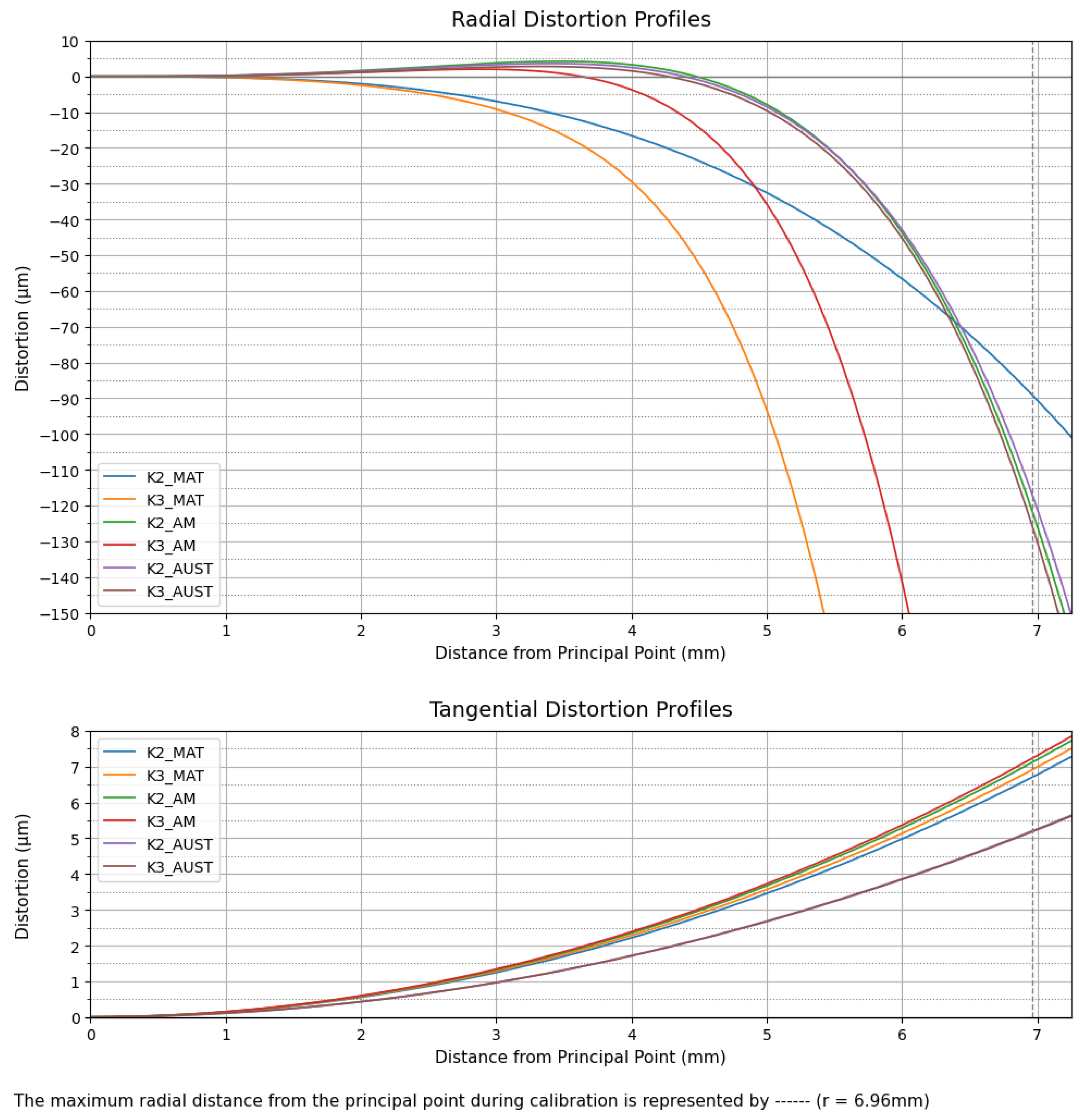
4.1.2. Interior Orientation
4.1.3. Relative Orientation
4.2. InfraRed Thermography 3D-Data Fusion (IRT-3DDF)
5. Conclusions
Author Contributions
Funding
Data Availability Statement
Acknowledgments
Conflicts of Interest
References
- Remondino, F.; Fraser, C. Digital Camera Calibration Methods: Considerations and Comparisons. In Proceedings of the ISPRS Commission V Symposium ‘Image Engineering and Vision Metrology’, Dresden, Germany, 25–27 September 2006; pp. 266–272. [Google Scholar] [CrossRef]
- Usamentiaga, R.; Garcia, D.; Ibarra-Castanedo, C.; Maldague, X. Highly Accurate Geometric Calibration for Infrared Cameras using Inexpensive Calibration Targets. Measurement 2017, 112, 105–116. [Google Scholar] [CrossRef]
- Fryskowska-Skibniewska, A.; Delis, P.; Kedzierski, M.; Matusiak, D. The Conception of Test Fields for Fast Geometric Calibration of the FLIR VUE PRO Thermal Camera for Low-Cost UAV Applications. Sensors 2022, 22, 2468. [Google Scholar] [CrossRef] [PubMed]
- St-Laurent, L.; Mikhnevich, M.; Bubel, A.; Prévost, D. Passive Calibration Board for Alignment of VIS-NIR, SWIR and LWIR Images. In Proceedings of the 13th International Conference on Quantitative InfraRed Thermography (QIRT 2016), Gdansk, Poland, 4–8 July 2016; pp. 777–784. [Google Scholar] [CrossRef]
- Swamidoss, I.N.; Bin Amro, A.; Sayadi, S. Systematic Approach for Thermal Imaging Camera Calibration for Machine Vision Applications. Optik 2021, 247, 168039. [Google Scholar] [CrossRef]
- Kubota, Y.; Ke, Y.; Hayakawa, T.; Moko, Y.; Ishikawa, M. Optimal Material Search for Infrared Markers under Non-Heating and Heating Conditions. Sensors 2021, 21, 6527. [Google Scholar] [CrossRef]
- Luhmann, T.; Fraser, C.; Maas, H.G. Sensor Modelling and Camera Calibration for Close-Range Photogrammetry. ISPRS J. Photogramm. Remote Sens. 2016, 115, 37–46. [Google Scholar] [CrossRef]
- Rankin, A.; Huertas, A.; Matthies, L.; Bajracharya, M.; Assad, C.; Brennan, S.; Bellutta, P.; Sherwin, G.W. Unmanned Ground Vehicle Perception Using Thermal Infrared Cameras. In Proceedings of the International Society for Optical Engineering, Orlando, FL, USA, 25–29 April 2011; Volume 8045, p. 804503. [Google Scholar] [CrossRef]
- Sun, S.; Wei, W.; Yuan, X.; Zhou, R. Research on Calibration Methods of Long-Wave Infrared Camera and Visible Camera. J. Sens. 2022, 2022, 8667606. [Google Scholar] [CrossRef]
- Bison, P.; Bortolin, A.; Cadelano, G.; Ferrarini, G.; Furlan, K.; Grinzato, E. Geometrical Correction and Photogrammetric Approach in Thermographic Inspection of Buildings. In Proceedings of the 11th International Conference on Quantitative InfraRed Thermography (QIRT 2012), Naples, Italy, 11–14 June 2012; pp. 1–9. [Google Scholar] [CrossRef]
- Harguess, J.; Strange, S. Infrared Stereo Calibration for Unmanned Ground Vehicle Navigation. In Proceedings of the International Society for Optical Engineering, Baltimore, MD, USA, 5–9 May 2014; Volume 9084, p. 90840S. [Google Scholar] [CrossRef]
- Motayyeb, S.; Samadzedegan, F.; Dadrass Javan, F.; Hosseinpour, H. Fusion of UAV-based Infrared and Visible Images for Thermal Leakage Map Generation of Building Façades. Heliyon 2023, 9, e14551. [Google Scholar] [CrossRef]
- ElSheikh, A.; Abu-Nabah, B.A.; Hamdan, M.O.; Tian, G.Y. Infrared Camera Geometric Calibration: A Review and a Precise Thermal Radiation Checkerboard Target. Sensors 2023, 23, 3479. [Google Scholar] [CrossRef]
- Zhang, C.; Zou, Y.; Dimyadi, J.; Chang, R. Thermal-textured BIM Generation for Building Energy Audit with UAV Image Fusion and Histogram-based Enhancement. Energy Build. 2023, 301, 113710. [Google Scholar] [CrossRef]
- Roshan, M.C.; Isaksson, M.; Pranata, A. A Geometric Calibration Method for Thermal Cameras using a ChArUco Board. Infrared Phys. Technol. 2024, 138, 105219. [Google Scholar] [CrossRef]
- Garrido-Jurado, S.; Muñoz-Salinas, R.; Madrid-Cuevas, F.; Marín-Jiménez, M. Automatic Generation and Detection of Highly Reliable Fiducial Markers under Occlusion. Pattern Recognit. 2014, 47, 2280–2292. [Google Scholar] [CrossRef]
- Westfeld, P.; Mader, D.; Maas, H.G. Generation of TIR-attributed 3D Point Clouds from UAV-based Thermal Imagery. Photogramm.—Fernerkund.—Geoinf. 2015, 2015, 381–393. [Google Scholar] [CrossRef]
- Yastikli, N.; Guler, E. Performance Evaluation of Thermographic Cameras for Photogrammetric Measurements. Int. Arch. Photogramm. Remote Sens. Spatial Inf. Sci. 2013, XL-1/W1, 383–387. [Google Scholar] [CrossRef]
- Rizzi, A.; Voltolini, F.; Girardi, S.; Gonzo, L.; Remondino, F. Digital Preservation, Documentation and Analysis of Paintings, Monuments and Large Cultural Heritage with Infrared Technology, Digital Cameras and Range Sensors. In Proceedings of the 21st International CIPA Symposium, Athens, Greece, 1–6 October 2007; pp. 1–6. [Google Scholar]
- Rangel, J.; Soldan, S. 3D Thermal Imaging: Fusion of Thermography and Depth Cameras. In Proceedings of the 12th International Conference on Quantitative InfraRed Thermography (QIRT 2014), Bordeaux, France, 7–11 July 2014; pp. 1–10. [Google Scholar] [CrossRef]
- Adán, A.; Prado, T.; Prieto, S.A.; Quintana, B. Fusion of Thermal Imagery and LiDAR Data for Generating TBIM Models. In Proceedings of the IEEE SENSORS 2017, Glasgow, UK, 29 October–1 November 2017; pp. 1–3. [Google Scholar] [CrossRef]
- Luhmann, T.; Piechel, J.; Roelfs, T. Geometric Calibration of Thermographic Cameras. In Thermal Infrared Remote Sensing; Kuenzer, C., Dech, S., Eds.; Springer: Dordrecht, The Netherlands, 2013; Volume 17, pp. 27–42. [Google Scholar] [CrossRef]
- Dlesk, A.; Vach, K.; Pavelka, K. Transformations in the Photogrammetric Co-Processing of Thermal Infrared Images and RGB Images. Sensors 2021, 21, 5061. [Google Scholar] [CrossRef]
- Sutherland, N.; Marsh, S.; Priestnall, G.; Bryan, P.; Mills, J. InfraRed Thermography and 3D-Data Fusion for Architectural Heritage: A Scoping Review. Remote Sens. 2023, 15, 2422. [Google Scholar] [CrossRef]
- Alba, M.I.; Barazzetti, L.; Scaioni, M.; Rosina, E.; Previtali, M. Mapping Infrared Data on Terrestrial Laser Scanning 3D Models of Buildings. Remote Sens. 2011, 3, 1847–1870. [Google Scholar] [CrossRef]
- Ham, Y.; Golparvar-Fard, M. An Automated Vision-Based Method for Rapid 3D Energy Performance Modeling of Existing Buildings Using Thermal and Digital Imagery. Adv. Eng. Inform. 2013, 27, 395–409. [Google Scholar] [CrossRef]
- Patrucco, G.; Cortese, G.; Giulio Tonolo, F.; Spanò, A. Thermal and Optical Data Fusion Supporting Built Heritage Analyses. Int. Arch. Photogramm. Remote Sens. Spatial Inf. Sci. 2020, XLIII-B3-2020, 619–626. [Google Scholar] [CrossRef]
- Adamopoulos, E.; Volinia, M.; Girotto, M.; Rinaudo, F. Three-Dimensional Thermal Mapping from IRT Images for Rapid Architectural Heritage NDT. Buildings 2020, 10, 187. [Google Scholar] [CrossRef]
- Lecomte, V.; Macher, H.; Landes, T. Combination of Thermal Infrared Images and Laserscanning Data for 3D Thermal Point Cloud Generation on Buildings and Trees. Int. Arch. Photogramm. Remote Sens. Spatial Inf. Sci. 2022, XLVIII-2/W1-2022, 129–136. [Google Scholar] [CrossRef]
- Macher, H.; Landes, T. Combining TIR Images and Point Clouds for Urban Scenes Modelling. Int. Arch. Photogramm. Remote Sens. Spatial Inf. Sci. 2022, XLIII-B2-2022, 425–431. [Google Scholar] [CrossRef]
- Lerma, J.L.; Navarro, S.; Cabrelles, M.; Seguí, A.E. Camera Calibration with Baseline Distance Constraints. Photogramm. Rec. 2010, 25, 140–158. [Google Scholar] [CrossRef]
- Ursine, W.; Calado, F.; Teixeira, G.; Diniz, H.; Silvino, S.; De Andrade, R. Thermal/Visible Autonomous Stereo Visio System Calibration Methodology for Non-controlled Environments. In Proceedings of the 11th International Conference on Quantitative InfraRed Thermography (QIRT 2012), Naples, Italy, 11–14 June 2012; pp. 1–11. [Google Scholar] [CrossRef]
- Fraser, C. Automatic Camera Calibration in Close Range Photogrammetry. Photogramm. Eng. Remote Sens. 2013, 79, 381–388. [Google Scholar] [CrossRef]
- Hastedt, H.; Luhmann, T. Investigations on the Quality of the Interior Orientation and its Impact in Object Space for UAV Photogrammetry. Int. Arch. Photogramm. Remote Sens. Spatial Inf. Sci. 2015, XL-1/W4, 321–328. [Google Scholar] [CrossRef]
- Duran, Z.; Atik, M.E. Accuracy Comparison of Interior Orientation Parameters from Different Photogrammetric Software and Direct Linear Transformation Method. Int. J. Eng. Geosci. 2021, 6, 74–80. [Google Scholar] [CrossRef]
- ASTM E1933-14(2018); Practice for Measuring and Compensating for Emissivity Using Infrared Imaging Radiometers. ASTM International: West Conshohocken, PA, USA, 2022. [CrossRef]
- Brown, D.C. Close-Range Camera Calibration. Photogramm. Eng. 1971, 37, 855–866. [Google Scholar]
- Workswell s.r.o. Workswell WIRIS Pro Datasheet. 2021. Available online: https://my.workswell.eu/download/file/33/en (accessed on 4 February 2025).
- Luhmann, T.; Robson, S.; Kyle, S. (Eds.) Close-Range Photogrammetry: Principles, Methods and Applications, 2nd ed.; Whittles Publishing: Dunbeath, UK, 2006. [Google Scholar]
- Perda, G.; Morelli, L.; Remondino, F.; Fraser, C.; Luhmann, T. Analyzing Target-, Handcrafted- and Learning-Based Methods for Automated 3D Measurement and Modelling. Int. Arch. Photogramm. Remote Sens. Spatial Inf. Sci. 2024, XLVIII-2/W7-2024, 105–112. [Google Scholar] [CrossRef]
- Zhang, Z. A Flexible New Technique for Camera Calibration. IEEE Trans. Pattern Anal. Mach. Intell. 2000, 22, 1330–1334. [Google Scholar] [CrossRef]
- Wan, Q.; Brede, B.; Smigaj, M.; Kooistra, L. Factors Influencing Temperature Measurements from Miniaturized Thermal Infrared (TIR) Cameras: A Laboratory-Based Approach. Sensors 2021, 21, 8466. [Google Scholar] [CrossRef]
- Kelly, J.; Kljun, N.; Olsson, P.O.; Mihai, L.; Liljeblad, B.; Weslien, P.; Klemedtsson, L.; Eklundh, L. Challenges and Best Practices for Deriving Temperature Data from an Uncalibrated UAV Thermal Infrared Camera. Remote Sens. 2019, 11, 567. [Google Scholar] [CrossRef]
- Jin, Y.; Mishkin, D.; Mishchuk, A.; Matas, J.; Fua, P.; Yi, K.M.; Trulls, E. Image Matching Across Wide Baselines: From Paper to Practice. Int. J. Comput. Vis. 2020, 129, 517–547. [Google Scholar] [CrossRef]
- Velesaca, H.O.; Bastidas, G.; Rouhani, M.; Sappa, A.D. Multimodal Image Registration Techniques: A Comprehensive Survey. Multimed. Tools Appl. 2024, 83, 63919–63947. [Google Scholar] [CrossRef]
- Elias, M.; Weitkamp, A.; Eltner, A. Multi-Modal Image Matching to Colorize a SLAM-based Point Cloud with Arbitrary Data from a Thermal Camera. ISPRS Open J. Photogramm. Remote Sens. 2023, 9, 100041. [Google Scholar] [CrossRef]
- Morelli, L.; Ioli, F.; Maiwald, F.; Mazzacca, G.; Menna, F.; Remondino, F. Deep-Image-Matching: A Toolbox for Multiview Image Matching of Complex Scenarios. Int. Arch. Photogramm. Remote Sens. Spatial Inf. Sci. 2024, XLVIII-2/W4-2024, 309–316. [Google Scholar] [CrossRef]
- DeTone, D.; Malisiewicz, T.; Rabinovich, A. SuperPoint: Self-Supervised Interest Point Detection and Description. In Proceedings of the IEEE/CVF Conference on Computer Vision and Pattern Recognition Workshops (CVPRW), Salt Lake City, UT, USA, 18–22 June 2018; pp. 337–349. [Google Scholar] [CrossRef]
- Lindenberger, P.; Sarlin, P.E.; Pollefeys, M. LightGlue: Local Feature Matching at Light Speed. In Proceedings of the IEEE/CVF International Conference on Computer Vision (ICCV), Paris, France, 1–6 October 2023; pp. 17581–17592. [Google Scholar] [CrossRef]
- Schonberger, J.L.; Frahm, J.M. Structure-from-Motion Revisited. In Proceedings of the IEEE Conference on Computer Vision and Pattern Recognition (CVPR), Las Vegas, NV, USA, 27–30 June 2016; pp. 4104–4113. [Google Scholar] [CrossRef]
- Sledz, A.; Heipke, C. Joint Bundle Adjustment of Thermal Infra-Red and Optical Images Based on Multimodal Matching. Int. Arch. Photogramm. Remote Sens. Spatial Inf. Sci. 2022, XLIII-B1-2022, 157–165. [Google Scholar] [CrossRef]
- Williams, J.; Corvaro, F.; Vignola, J.; Turo, D.; Marchetti, B.; Vitali, M. Application of Non-Invasive Active Infrared Thermography for Delamination Detection in Fresco. Int. J. Therm. Sci. 2022, 171, 107185. [Google Scholar] [CrossRef]
- Zhang, J.; Zhang, S.; Peng, G.; Zhang, H.; Wang, D. 3DRadar2ThermalCalib: Accurate Extrinsic Calibration between a 3D mmWave Radar and a Thermal Camera Using a Spherical-Trihedral. In Proceedings of the 25th International Conference on Intelligent Transportation Systems (ITSC), Macau, China, 8–12 October 2022; pp. 2744–2749. [Google Scholar] [CrossRef]
- Lagüela, S.; González-Jorge, H.; Armesto, J.; Arias, P. Calibration and Verification of Thermographic Cameras for Geometric Measurements. Infrared Phys. Technol. 2011, 54, 92–99. [Google Scholar] [CrossRef]
- Adán, A.; Pérez, V.; Vivancos, J.L.; Aparicio-Fernández, C.; Prieto, S.A. Proposing 3D Thermal Technology for Heritage Building Energy Monitoring. Remote Sens. 2021, 13, 1537. [Google Scholar] [CrossRef]
- Clarke, T.A.; Wang, X.; Fryer, J.G. The Principal Point and CCD Cameras. Photogramm. Rec. 1998, 16, 293–312. [Google Scholar] [CrossRef]
- Senn, J.A.; Mills, J.; Walsh, C.L.; Addy, S.; Peppa, M.V. On-Site Geometric Calibration of RPAS Mounted Sensors for SfM Photogrammetric Geomorphological Surveys. Earth Surf. Processes Landforms 2022, 47, 1615–1634. [Google Scholar] [CrossRef]
- Daakir, M.; Zhou, Y.; Pierrot Deseilligny, M.; Thom, C.; Martin, O.; Rupnik, E. Improvement of Photogrammetric Accuracy by Modeling and Correcting the Thermal Effect on Camera Calibration. ISPRS J. Photogramm. Remote Sens. 2019, 148, 142–155. [Google Scholar] [CrossRef]
- Tejedor, B.; Lucchi, E.; Bienvenido-Huertas, D.; Nardi, I. Non-Destructive Techniques (NDT) for the Diagnosis of Heritage Buildings: Traditional Procedures and Futures Perspectives. Energy Build. 2022, 263, 112029. [Google Scholar] [CrossRef]
- Adán, A.; Pérez, V.; Ramón, A.; Castilla, F.J. Correction of Temperature from Infrared Cameras for More Precise As-Is 3D Thermal Models of Buildings. Appl. Sci. 2023, 13, 6779. [Google Scholar] [CrossRef]


| Workswell WIRIS Pro Infrared Sensor (WWP) | |
| Resolution | 640× 512 pix |
| Sensor Size (FPA) | 10.88 × 8.71 mm |
| Pixel Size | 17.00 µm |
| Nominal Focal Length | 13.00 mm |
| Spectral Range (LWIR) | 7.5–13.5 µm |
| Temp. Sensitivity | 0.05 °C |
| Temp. Accuracy | ±2 °C |
| Workswell WIRIS Pro Visible Sensor (VIS) | |
| Resolution | 1920 × 1080 pix |
| Sensor Size (CMOS) | 5.23 × 2.94 mm |
| Pixel Size | 2.72 µm |
| Nominal Focal Length | 3.50 mm |
| Sony α 7R II (RGB1) | |
| Resolution | 7952× 5304 pix |
| Sensor Size (CMOS) | 35.90× 24.00 mm |
| Pixel Size | 4.50 µm |
| Nominal Focal Length | 35.00 mm |
| Nikon D750 (RGB2) | |
| Resolution | 6016× 4016 pix |
| Sensor Size (CMOS) | 35.90 × 24.00 mm |
| Pixel Size | 5.95 µm |
| Nominal Focal Length | 50.00 mm |
| Material | ||||
|---|---|---|---|---|
| 2D Board | DiBond® | 0.62 | 0.04 | 0.20 |
| UV-printing | 0.82 | 0.04 | ||
| 3D Field | Aluminium | 0.20 | 0.03 | 0.65 |
| Rubber | 0.85 | 0.05 |
| Coefficient | Intrinsics | 2D Board (MATLAB) | 3D Field (Agisoft Metashape | 3D Field (Australis) | |||
|---|---|---|---|---|---|---|---|
| Value | Value | Value | |||||
| f (mm) | 13.021 | 0.032 | 13.038 | 0.015 | 13.034 | 0.014 | |
| (pix) | 311.219 | 1.821 | 312.585 | 0.626 | 312.926 | 0.740 | |
| (pix) | 255.558 | 1.928 | 257.755 | 0.614 | 257.921 | 0.721 | |
| 0.044 | 0.009 | −0.043 | 0.004 | −0.039 | 0.003 | ||
| 0.005 | 0.054 | 0.368 | 0.014 | 0.347 | 0.013 | ||
| −0.000 | 0.001 | −0.001 | 0.000 | 0.000 | 0.000 | ||
| 0.001 | 0.001 | 0.000 | 0.000 | −0.000 | 0.000 | ||
| MRE (pix) | 0.50 | 0.16 | 0.12 | ||||
| (mm) | 3.20 | 3.25 | 2.06 | ||||
| f (mm) | 13.017 | 0.032 | 13.033 | 0.015 | 13.030 | 0.014 | |
| (pix) | 311.232 | 1.823 | 312.541 | 0.623 | 312.908 | 0.730 | |
| (pix) | 255.482 | 1.926 | 257.741 | 0.612 | 257.940 | 0.711 | |
| 0.055 | 0.017 | −0.031 | 0.008 | −0.031 | 0.008 | ||
| −0.177 | 0.247 | 0.247 | 0.078 | 0.270 | 0.073 | ||
| 0.791 | 1.047 | 0.350 | 0.221 | 0.214 | 0.204 | ||
| −0.000 | 0.001 | −0.001 | 0.000 | 0.000 | 0.000 | ||
| 0.001 | 0.001 | 0.000 | 0.000 | −0.000 | 0.000 | ||
| MRE (pix) | 0.50 | 0.16 | 0.12 | ||||
| (mm) | 3.65 | 3.25 | 2.08 | ||||
| Coefficient | Baseline | Parameters | 2D Board (MATLAB) | 3D Field (Agisoft Metashape) | 3D Field (Australis) | |||
|---|---|---|---|---|---|---|---|---|
| Value | Value | Value | ||||||
| VIS-WWP | X (mm) | −41.530 | 0.191 | −39.738 | 0.396 | −40.271 | 2.691 | |
| Y (mm) | −1.992 | 0.149 | 0.409 | 0.363 | −0.148 | 2.845 | ||
| Z (mm) | 0.309 | 0.114 | 1.142 | 0.219 | 6.124 | 1.456 | ||
| (°) | −0.080 | 0.013 | −0.092 | 0.008 | −0.175 | 0.073 | ||
| (°) | 0.579 | 0.016 | 0.717 | 0.009 | 0.701 | 0.071 | ||
| (°) | −0.080 | 0.010 | 0.001 | 0.005 | 0.000 | 0.021 | ||
| MRE (pix) | 0.76 | 0.55 | 0.22 | |||||
| (mm) | 4.48 | 3.20 | 2.32 | |||||
| RGB2-WWP | X (mm) | −184.464 | 0.331 | −183.659 | 0.629 | −183.084 | 1.493 | |
| Y (mm) | −0.216 | 0.241 | 1.501 | 0.578 | 1.242 | 2.023 | ||
| Z (mm) | 6.925 | 0.252 | 9.737 | 0.501 | 11.154 | 1.276 | ||
| (°) | 0.917 | 0.015 | 0.586 | 0.015 | 0.424 | 0.080 | ||
| (°) | 3.644 | 0.020 | 3.243 | 0.015 | 3.208 | 0.066 | ||
| (°) | −0.046 | 0.015 | −0.147 | 0.014 | −0.175 | 0.296 | ||
| MRE (pix) | 0.87 | 1.10 | 0.14 | |||||
| (mm) | 5.26 | 2.17 | 0.77 | |||||
| VIS-WWP | X (mm) | −41.503 | 0.191 | −39.721 | 0.395 | −40.540 | 2.889 | |
| Y (mm) | −1.990 | 0.149 | 0.406 | 0.362 | −0.614 | 2.895 | ||
| Z (mm) | 0.371 | 0.114 | 1.272 | 0.219 | −1.338 | 1.094 | ||
| (°) | −0.080 | 0.013 | −0.092 | 0.008 | 0.025 | 0.075 | ||
| (°) | 0.579 | 0.016 | 0.713 | 0.009 | 0.715 | 0.072 | ||
| (°) | −0.080 | 0.010 | 0.001 | 0.005 | −0.007 | 0.019 | ||
| MRE (pix) | 0.76 | 0.55 | 0.29 | |||||
| (mm) | 4.48 | 3.20 | 3.54 | |||||
| RGB2-WWP | X (mm) | −184.446 | 0.331 | −183.644 | 0.629 | −183.143 | 1.495 | |
| Y (mm) | −0.215 | 0.241 | 1.490 | 0.578 | 1.064 | 2.143 | ||
| Z (mm) | 7.017 | 0.252 | 9.340 | 0.502 | 11.132 | 1.263 | ||
| (°) | 0.917 | 0.014 | 0.565 | 0.015 | 0.418 | 0.085 | ||
| (°) | 3.644 | 0.020 | 3.267 | 0.015 | 3.213 | 0.068 | ||
| (°) | −0.046 | 0.015 | −0.146 | 0.014 | −0.154 | 0.311 | ||
| MRE (pix) | 0.87 | 1.10 | 0.14 | |||||
| (mm) | 5.26 | 2.11 | 0.76 | |||||
| Parameters | RMSERGB1 (mm) | MREWWP (pix) | RMSEWWP (mm) | ||||
|---|---|---|---|---|---|---|---|
| X | Y | Z | TOT | ||||
| Self-Calibration | 2.86 | 0.32 | 4.02 | 16.31 | 9.03 | 19.07 | |
| MATLAB | 2.59 | 0.40 | 3.88 | 14.11 | 10.55 | 18.04 | |
| 2.60 | 0.31 | 3.98 | 12.39 | 8.63 | 15.62 | ||
| Agisoft Metashape | 2.44 | 0.27 | 2.72 | 5.74 | 6.12 | 8.82 | |
| 2.47 | 0.28 | 2.45 | 6.91 | 5.69 | 9.28 | ||
| Australis | 2.32 | 0.29 | 3.05 | 5.44 | 6.35 | 8.89 | |
| 2.19 | 0.29 | 3.06 | 5.60 | 6.28 | 8.95 | ||
| Parameters | RMSE VIS-WWP (mm) | RMSE RGB2-WWP (mm) | |||
|---|---|---|---|---|---|
| VIS | WWP | RGB2 | WWP | ||
| Self-Calibration | 2.43 | 4.30 | 1.46 | 1.42 | |
| MATLAB | 1.49 | 5.04 | 2.20 | 8.72 | |
| 1.51 | 5.01 | 2.17 | 8.82 | ||
| Agisoft Metashape | 2.72 | 4.12 | 1.26 | 1.87 | |
| 2.74 | 4.24 | 1.26 | 1.89 | ||
| Australis | 2.25 | 3.83 | 1.26 | 1.58 | |
| 2.28 | 3.95 | 1.26 | 1.65 | ||
Disclaimer/Publisher’s Note: The statements, opinions and data contained in all publications are solely those of the individual author(s) and contributor(s) and not of MDPI and/or the editor(s). MDPI and/or the editor(s) disclaim responsibility for any injury to people or property resulting from any ideas, methods, instructions or products referred to in the content. |
© 2025 by the authors. Licensee MDPI, Basel, Switzerland. This article is an open access article distributed under the terms and conditions of the Creative Commons Attribution (CC BY) license (https://creativecommons.org/licenses/by/4.0/).
Share and Cite
Sutherland, N.; Marsh, S.; Remondino, F.; Perda, G.; Bryan, P.; Mills, J. Geometric Calibration of Thermal Infrared Cameras: A Comparative Analysis for Photogrammetric Data Fusion. Metrology 2025, 5, 43. https://doi.org/10.3390/metrology5030043
Sutherland N, Marsh S, Remondino F, Perda G, Bryan P, Mills J. Geometric Calibration of Thermal Infrared Cameras: A Comparative Analysis for Photogrammetric Data Fusion. Metrology. 2025; 5(3):43. https://doi.org/10.3390/metrology5030043
Chicago/Turabian StyleSutherland, Neil, Stuart Marsh, Fabio Remondino, Giulio Perda, Paul Bryan, and Jon Mills. 2025. "Geometric Calibration of Thermal Infrared Cameras: A Comparative Analysis for Photogrammetric Data Fusion" Metrology 5, no. 3: 43. https://doi.org/10.3390/metrology5030043
APA StyleSutherland, N., Marsh, S., Remondino, F., Perda, G., Bryan, P., & Mills, J. (2025). Geometric Calibration of Thermal Infrared Cameras: A Comparative Analysis for Photogrammetric Data Fusion. Metrology, 5(3), 43. https://doi.org/10.3390/metrology5030043