New Types of Derivative Non-linear Schrödinger Equations Related to Kac–Moody Algebra ${\mathit{A}}_{\mathbf{2}}^{\mathbf{\left(}\mathbf{1}\mathbf{\right)}}$

Abstract

We derive a new system of integrable derivative non-linear Schrödinger equations with an L operator, quadratic in the spectral parameter with coefficients belonging to the Kac–Moody algebra $A_2^{\left(1\right)}$. The construction of the fundamental analytic solutions of L is outlined and they are used to introduce the scattering data, thus formulating the scattering problem for the Lax pair $L,M$.

1. Introduction

Since the seminal papers [1,2], nonlinear PDEs solvable by the inverse scattering transform (IST) became of interest for both physicists and mathematicians. One such equation is the non-linear Schrödinger equation (NLS) [3,4] which admits multi-component generalizations, the most famous being the Manakov model [5]. All such generalizations can be associated with an $L,M$ pair, such that the L operator is linear in the spectral parameter $\lambda$. In fact, most of the efforts went into studying systems with such linear L operators. This is in part due to the fact that such operators are zero-curvature representations (ZCR) of scalar Lax pairs. Another reason is the fact that the study of L operators, polynomial in the spectral parameter (often called polynomial bundles or polynomial pencils), presents numerous challenges.

The first known example of an equation related to a Lax operator with quadratic dependence on the spectral parameter is a variation in the NLS equation known as the derivative non-linear Schrödinger (dNLS) equation. In fact, there are three equivalent models that fall under that name:

• The Kaup–Newell Equation [6], also known as dNLS-I:

  $${\partial }_{t}q+{\partial }_x^{2}q\pm i{\partial }_x\left({q\left|q\right|}^2\right)=0.$$

  (1)
• The Chen–Lee–Liu Equation [7], also known as dNLS-II:

  $$i{\partial }_{t}q+{\partial }_x^{2}q-{\left|q\right|}^2{\partial }_{x}q=0.$$

  (2)
• The Gerdjikov–Ivanov Equation [8], also known as dNLS-III:

  $$i{\partial }_{t}q+{\partial }_x^{2}q-{\left|q\right|}^2{\partial }_x{q}^{\ast }+\frac{1}{2}{\left|q\right|}^{4}q=0,$$

  (3)

  where * denotes complex conjugation.

They are equivalent in the sense that they can be related to one another with a suitable gauge transformation.

Most integrable equations with one component usually allow multi-component generalizations by considering Lax pairs with potentials in some semisimple Lie algebra $\mathfrak{g}$. In general, without imposing additional conditions on the form of the Lax pair, the resulting equations will contain a large number of independent functions, which limits their applicability. One way out of this difficulty is to impose an additional condition, called a reduction, using a finite order automorphism $\phi$. The reduction, that gives the lowest number of components, is a Coxeter reduction; i.e., $\phi$ is a Coxeter automorphism of the corresponding Lie algebra $\mathfrak{g}$. Reductions form a group, called the reduction group. For the case of a Coxeter reduction, this group is simply ${\mathbb{Z}}_h$ (cyclic group of order h), where h is the Coxeter number of the corresponding algebra. Reductions of Lax pairs and their theory were studied extensively by Mikhailov, and the reader is encouraged to read his original article where the subject is thoroughly examined [9].

Some multi-component generalizations of the dNLS equation can be derived by considering an $L,M$ pair with potentials in the simple Lie algebra $A_r\simeq sl(r+1)$, such that L is linear and M is quadratic in the spectral parameter $\lambda$. Additionally, in order to reduce the number of components, usually a ${\mathbb{Z}}_n$ reduction is imposed. Such models were considered in [10].

Formally, the potentials of $L,M$ pairs with a Coxeter reduction can be viewed as elements of Kac–Moody algebras. Such an approach was chosen by Drinfeld and Sokolov [11,12] where integrable models, related to low-rank Kac–Moody algebras were studied (again, only for L operators linear in the spectral parameter $\lambda$). The cases for $A_r^{\left(1\right)}$ and $D_4^{\left(k\right)}$ can be found in [13,14]. There are, however, no known models related to Kac–Moody algebras with L being polynomial in $\lambda$.

Formulating the scattering problem for the linear Lax operator was treated with mathematical rigor for the general case by Beals and Coifman [15], and for the case of potentials in semisimple Lie algebras (which includes the case of a Coxeter reduction) by Gerdjikov and Yanovski [16,17].

Studying exactly solvable models related to the polynomial case presents some difficulties. First, there is the question of the parametrization of the Lax operators. The second is the formulation of the scattering problem, starting with the introduction of the fundamental analytic solutions (FAS). Note that there have been some advances in the study of polynomial Lax operators. A significant contribution can be found in [18], where a general approach for parametrizing the Lax operators is formulated. The main idea is to start from a multiplicative Riemann–Hilbert problem (RHP), with everything else following from there. The article also contains examples of N-wave equations with a ${\mathbb{Z}}_2$ reduction group and dNLS-type equations related to symmetric spaces.

The aim of this paper is to outline the general methodology in solving the mentioned difficulties for the case of the quadratic Lax operator related to Kac–Moody algebra $A_2^{\left(1\right)}$, which results in a set of dNLS equations, for which the scattering problem is formulated. This can be considered as a natural continuation of the work performed in [18]. The chosen approach is slightly different: we will start with a Lax representation, then formulate the FAS for the relevant pair of Lax operators, show that they satisfy a multiplicative RHP, and then formulate the scattering problem and find a minimal set of scattering data.

A word on terminology—formally, a Lax pair is a pair of scalar operators and not their matrix analogs, but we will not make this distinction here and will refer to any $L,M$ pair as a Lax pair and the L operator as a Lax operator. The reader is assumed to have some familiarity with the history and basic theory of integrable systems—for an introduction, see [19].

This paper is structured as follows: Section 1 is this introduction; Section 2 contains the necessary preliminaries from the theory of simple Lie algebras; Section 3 is devoted to the recursion relations resulting from the compatibility condition of the $L,M$ pair; Section 4 presents the resulting dNLS-type equations; Section 5 introduces the FAS and formulates the scattering problem; Section 6 studies the time evolution of the scattering matrix; and Section 7 contains some concluding remarks. The Appendix is divided as follows: Appendix A introduces the Cartan–Weyl basis for the simple lie algebra $A_2$; Appendix B contains the basis for the Kac–Moody algebra $A_2^{\left(1\right)}$; and Appendix C derives the expression for the inverse of $a{d}_J$ (which is frequently used throughout the text).

2. Preliminaries

The reader is assumed to have basic knowledge of the theory of simple Lie algebras. Some classical textbooks on the theory of Lie algebras, both finite and infinite dimensional, are [20,21,22].

Assume that $\mathfrak{g}$ is a finite-dimensional simple Lie algebra over the field of complex numbers $\mathbb{C}$. Let ${\mathrm{ad}}_X$ denote the linear operator defined by

$${\mathrm{ad}}_X\left(Y\right)=\left[X,Y\right],X,Y\in \mathfrak{g},$$

(4)

where $[,]$ denotes the Lie bracket in $\mathfrak{g}$. This operator has a kernel and can only be inverted on its image. We denote that inverse by ${\mathrm{ad}}_X^{-1}$. If X is diagonalizable then ${\mathrm{ad}}_X^{-1}$ can be expressed as a polynomial of ${\mathrm{ad}}_X$. We will also need the Killing–Cartan form on $\mathfrak{g}$, usually denoted $⟨,⟩$, which is defined by

$$⟨X,Y⟩=\mathrm{tr}\left({\mathrm{ad}}_X{\mathrm{ad}}_Y\right),$$

(5)

where $\mathrm{t}\mathrm{r}$ denotes the trace. Note that for any simple Lie algebras, any invariant symmetric bilinear form on $\mathfrak{g}$ is proportional to this Killing form. This simplifies things, since in any representation of $\mathfrak{g}$, we can use the form (ignoring the proportionality constant)

$$⟨X,Y⟩=\mathrm{tr}\left(XY\right).$$

(6)

Now, assume that $\phi$ is an automorphism of $\mathfrak{g}$ of finite order. If $\phi$ can be represented as

$$\phi \left(X\right)=e^{F}X{e}^{-F}$$

(7)

for some generator F, then it is an inner automorphism. An outer automorphism is one which is not inner. The set of outer automorphisms of $\mathfrak{g}$ is equivalent (up to a conjugation with an inner automorphism) to the symmetries of the Dynkin diagram of $\mathfrak{g}$.

An automorphism is said to be a Coxeter automorphism if its invariant eigenspace is Abelian and the automorphism is of minimal order h, with h being called the Coxeter number of the algebra.

Any finite order automorphism $\phi$ introduces a grading in $\mathfrak{g}$ by the condition

$$\mathfrak{g}=\underset{k=0}{\overset{s-1}{\oplus }}{\mathfrak{g}}^{\left(k\right)},$$

(8)

such that

$$\left[{\mathfrak{g}}^{\left(k\right)},{\mathfrak{g}}^{\left(l\right)}\right]\subset {\mathfrak{g}}^{(k+l)},\phi \left(X\right)={\omega }^{k}X,\omega =exp\left(\frac{2\pi i}{s}\right),\forall X\in {\mathfrak{g}}^{\left(k\right)},$$

(9)

where s is the order of $\phi$ and $k+l$ is taken modulo s. Let us define

$$\begin{array}{cc}\hfill \mathfrak{g}[\lambda ,{\lambda }^{-1}]& =\left\{\sum _{i=n}^m{v}_i{\lambda }^i:v_i\in \mathfrak{g},n,m\in \mathbb{Z}\right\},\hfill \\ \hfill f\left(\lambda \right)& =\left\{\sum _{i=0}^m{f}_i{\lambda }^i:f_i\in \mathfrak{g},m\in \mathbb{Z}\right\}.\hfill \end{array}$$

(10)

There is a natural Lie algebraic structure on $\mathfrak{g}[\lambda ,{\lambda }^{-1}]$. Let $\phi$ be an automorphism of $\mathfrak{g}$ of order s. Then

$$L(\mathfrak{g},\phi )=\left\{f\in \mathfrak{g}[\lambda ,{\lambda }^{-1}]:\phi \left(f\left(\lambda \right)\right)=f\left(\lambda exp\left(\frac{2\pi i}{s}\right)\right)\right\}.$$

(11)

$L(\mathfrak{g},\phi )$ is a Lie subalgebra of $\mathfrak{g}[\lambda ,{\lambda }^{-1}]$.

If $\mathfrak{g}$ is simple and $\phi$ is a Coxeter automorphism then $L(\mathfrak{g},\phi )$ is called a Kac–Moody algebra.

Note that when considering finite-dimensional Lie algebras, a Coxeter automorphism is an inner automorphism. When dealing with Kac–Moody algebras, the Coxeter automorphism can be an outer automorphism of the underlying simple Lie algebra $\mathfrak{g}$. This usually means that we have two types of Kac–Moody algebras—twisted and untwisted (there exists one notable exception, the algebra $D_4^{\left(3\right)}$). When the Coxeter automorphism is an outer automorphism of $\mathfrak{g}$, then the corresponding Kac–Moody algebra is called twisted; otherwise it is untwisted. Untwisted Kac–Moody algebras are usually denoted by an upper index $\left(1\right)$, while the twisted type is denoted by an upper index $\left(2\right)$, with this number being called the height of the Kac–Moody algebra. To make this more precise, consider that every automorphism $\phi$ can be uniquely written as $\phi =\psi \circ {\phi }_{\tau }$ where $\psi$ is an inner automorphism and ${\phi }_{\tau }$ is given by

$${\phi }_{\tau }\left(E_{{\alpha }_i}\right)=E_{\tau \left({\alpha }_i\right)}$$

(12)

with $\tau$ being a permutation of the simple roots that preserves the symmetry of the Dynkin diagram of $\mathfrak{g}$; i.e., it is an automorphism of the Dynkin diagram. Then the order of ${\phi }_{\tau }$ is the height of $L(\mathfrak{g},\phi )$. It is obvious that Kac–Moody algebras are graded algebras. Note that commonly the central extension of $L(\mathfrak{g},\phi )$ is called a Kac–Moody algebra, with the definitions given above being the ones used in [11,12].

In this paper, we will consider the equations related to $L(A_2,C)$, usually denoted by $A_2^{\left(1\right)}$. The Coxeter number of $A_2^{\left(1\right)}$ is 3, its rank is 2, and its exponents are $1,2$ [11,20]. We will use the typical representation (defining module) of $A_2\simeq sl\left(3\right)$, i.e., $3\times 3$ matrices with zero trace. The Lie bracket is then the commutator $[X,Y]=XY-YX$. The Coxeter automorphism C can be represented as

$$C\left(X\right)=cX{c}^{-1},$$

(13)

where the matrix c is given by

$$c=\left(\begin{array}{ccc}0& 0& 1\\ 1& 0& 0\\ 0& 1& 0\end{array}\right).$$

(14)

It introduces a grading in $A_2$ via (9). The basis is (the explicit form is given in the Appendix A):

$$\begin{array}{cc}\hfill {\mathcal{E}}_{\alpha }^{\left(k\right)}& =\sum _{s=0}^{h-1}{\omega }^{-sk}{C}^s\left(E_{\alpha }\right),{\mathcal{H}}_j^{\left(k\right)}=\sum _{s=0}^{h-1}{\omega }^{-sk}{C}^s\left(H_j\right),\hfill \\ \hfill & {\mathcal{E}}_{\alpha }^{\left(k\right)}\in {\mathfrak{g}}^{\left(k\right)},{\mathcal{H}}_j^{\left(k\right)}\in {\mathfrak{g}}^{\left(k\right)},\omega =e^{i\frac{2\pi }{3}}.\hfill \end{array}$$

(15)

Note that ${\mathcal{H}}_j^{\left(k\right)}$ is non-vanishing only if k is an exponent, i.e ${\mathcal{H}}_j^{\left(0\right)}=0$. Here, $H_j$ are the Cartan basis elements and $E_{\alpha }$ are the Weyl generators of $A_2$.

A note on notations—we will omit writing explicit dependence on $x,t$ or $\lambda$ when it is convenient and when there is no risk of confusion. Also, in order to avoid visual clutter, when needed, we will denote matrix inverse by “hat”; i.e., if F is an invertible matrix, then $\widehat{F}=F^{-1}$. Partial derivatives in x and t will be denoted by ${\partial }_x$ and ${\partial }_t$, respectively, and $11$ denotes the unity matrix.

3. Lax Pair and Recursion Relations

Consider a Lax pair given by

$$\begin{array}{cc}\hfill L& =i{\partial }_x+U_0(x,t)+\lambda U_1(x,t)-{\lambda }^{2}J,\hfill \\ \hfill M& =i{\partial }_t+V_0(x,t)+\lambda V_1(x,t)+{\lambda }^2{V}_2(x,t)+{\lambda }^3{V}_3(x,t)+{\lambda }^{4}K,\hfill \end{array}$$

(16)

where J and K are diagonal constant matrices with complex coefficients. Note that while in many cases L operators that are linear in the spectral parameter can be viewed as zero-curvature representations of scalar Lax operators, for the polynomial case there is no such analogy.

The parametrization of the coefficients of such Lax pair comes down to imposing the symmetry conditions, i.e., the Coxeter reduction and solving the recursion relations resulting from the ZCC. This can be summarized as follows:

• The potentials are elements of the corresponding eigenspaces of C

  $$\begin{array}{cc}\hfill U_0(x,t)\in {\mathfrak{g}}^{\left(0\right)}& ,U_1(x,t)\in {\mathfrak{g}}^{\left(1\right)},V_k(x,t)\in {\mathfrak{g}}^{(k mod 3)},\hfill \\ & K\in {\mathfrak{g}}^{\left(1\right)},J\in {\mathfrak{g}}^{\left(2\right)}.\hfill \end{array}$$

  (17)
  We will also assume that the potentials vanish at spatial infinity, i.e.,

  $$\underset{x\to \pm \infty }{lim}{U}_k(x,t)=0,\underset{x\to \pm \infty }{lim}{V}_k(x,t)=0.$$
  Usually, an ever more restrictive condition on the asymptotic behavior of the potentials is required. For the purposes of this paper, we will assume them to be Schwartz functions, but this might be too restrictive. This, of course, needs to be studied more rigorously and this will be accomplished in future works.
• The explicit form of the elements of L is:

  $$J={\mathcal{H}}_1^{\left(1\right)}=\left(\begin{array}{ccc}\omega & 0& 0\\ 0& {\omega }^2& 0\\ 0& 0& 1\end{array}\right),U_0=\left(\begin{array}{ccc}0& q_1& q_2\\ q_2& 0& q_1\\ q_1& q_2& 0\end{array}\right),U_1=\left(\begin{array}{ccc}0& {\omega }^2{q}_3& {\omega }^2{q}_4\\ \omega q_4& 0& q_3\omega \\ q_3& q_4& 0\end{array}\right)$$
• The choice of J determines the inverse of ${ad}_J$ to be (see Appendix C)

  $${\mathrm{ad}}_J^{-1}=-\frac{1}{27}{\mathrm{ad}}_J^5.$$

  (18)
• The elements of M are:

  $$K={\mathcal{H}}_1^{\left(2\right)}=\left(\begin{array}{ccc}{\omega }^2& 0& 0\\ 0& \omega & 0\\ 0& 0& 1\end{array}\right),V_k=v_1^{\left(k\right)}{\mathcal{E}}_{{\alpha }_1}^{\left(k\right)}+v_1^{\left(k\right)}{\mathcal{E}}_{{\alpha }_1+{\alpha }_2}^{\left(k\right)}+v_0^{\left(k\right)}{\mathcal{H}}_1^{\left(k\right)},$$

  where in the index k is taken as modulo 3.
• The zero-curvature condition $[L,M]=0$ leads to the following set of recursion relations with $N=4$:

  $$\begin{array}{cccc}\hfill & {\lambda }^{N+2}:\hfill & \hfill \left[J,K\right]& =0,\hfill \\ \hfill & {\lambda }^{N+1}:\hfill & \hfill \left[J,V_{N-1}\right]-\left[K,U_1\right]& =0,\hfill \\ \hfill & {\lambda }^N:\hfill & \hfill \left[J,V_{N-2}\right]-\left[K,U_0\right]-\left[U_1,V_{N-1}\right]& =0,\hfill \\ \hfill & {\lambda }^s:\hfill & \hfill i{\partial }_x{V}_s+\left[U_0,V_s\right]+\left[U_1,V_{s-1}\right]-\left[J,V_{s-2}\right]& =0,\hfill \\ \hfill & {\lambda }^1:\hfill & \hfill -i{\partial }_t{U}_1+i{\partial }_x{V}_1+\left[U_0,V_1\right]+\left[U_1,V_0\right]& =0,\hfill \\ \hfill & {\lambda }^0:\hfill & \hfill -i{\partial }_t{U}_0+i{\partial }_x{V}_0+\left[U_0,V_0\right]& =0.\hfill \end{array}$$

  (19)
• The recursion relations can be solved by noting that each $X\in \mathfrak{g}$ can be decomposed as

  $$X=X^{\perp }+X^{\parallel },{\mathrm{ad}}_J{X}^{\parallel }=[J,X^{\parallel }]=0,$$

  (20)

  i.e., $X^{\parallel }$ is “parallel” to J while $X^{\perp }$ is “orthogonal” to J.
• This leads to the following solutions:

  $$\begin{array}{cc}\hfill & V_{N-1}={\mathrm{ad}}_J^{-1}\left[K,U_1\right],\hfill \\ \hfill & V_{N-2}={\mathrm{ad}}_J^{-1}\left(\left[K,U_0\right]+\left[U_1,V_{N-1}\right]\right),\hfill \\ \hfill & V_{s-2}^{\perp }={\mathrm{ad}}_J^{-1}\left(i{\partial }_x{V}_s+\left[U_0,V_s^{\perp }\right]+\left[U_0,V_s^{\parallel }\right]+\left[U_1,V_{s-1}^{\perp }\right]+\left[U_1,V_{s-1}^{\parallel }\right]\right),\hfill \\ \hfill & V_s^{\parallel }=i{\partial }_x^{-1}\left({\left[U_0,V_s^{\perp }\right]}^{\parallel }+{\left[U_1,V_{s-1}^{\perp }\right]}^{\parallel }\right),\hfill \end{array}$$

  (21)

  where by ${\partial }_x^{-1}$ we denote the operator

  $${\partial }_x^{-1}f\left(x\right)={\int }_{-\infty }^{x}f\left(y\right)dy.$$
  Note that for any function vanishing at $-\infty$, this is equivalent to integrating and setting any constant of integration to zero. The above solutions to the recursion relations can be formalized with the help of recursion operators $\mathrm{\Lambda }$; see, for example [14,17]. However, calculating their explicit form in the case of polynomial Lax operators is more involved and writing their explicit form presents considerable difficulties.

The explicit form of the coefficients of $V_k$ is given by

$$\begin{array}{ccc}\hfill {v_1}^{\left(3\right)}& =-a{\omega }^2{q}_3,\hfill & \hfill {v_1}^{\left(2\right)}=-a{\omega }^2{q}_1-a\omega q_4^2,\\ \hfill {v_2}^{\left(3\right)}& =-a\omega q_4,\hfill & \hfill {v_2}^{\left(2\right)}=-a\omega q_1-a{\omega }^2{q}_4^2,\\ \hfill {v_3}^{\left(3\right)}& =0,\hfill & \hfill {v_3}^{\left(2\right)}=a{q}_3{q}_4.\end{array}$$

$$\begin{array}{cc}\hfill {v_1}^{\left(1\right)}& =a{\omega }^2{q}_4{q}_2-\frac{1}{\sqrt{3}}a{\partial }_x{q}_3,{v_2}^{\left(1\right)}=a\omega q_3{q}_1+\frac{1}{\sqrt{3}}a{\partial }_x{q}_4,\hfill \\ \hfill {v_3}^{\left(1\right)}& =-a\omega q_4{q}_1-a{\omega }^2{q}_3{q}_{@}-\frac{2}{3}a{q}_3^3-\frac{2}{3}a{q}_4^3.\hfill \end{array}$$

$$\begin{array}{cc}\hfill {v_1}^{\left(0\right)}& =a\left(-\frac{1}{\sqrt{3}}{\partial }_x{q}_1-\frac{2}{\sqrt{3}}{\omega }^2{q}_4{\partial }_x{q}_4-\frac{2}{3}{\omega }^2{q}_3^4-2\omega q_2{q}_3^2+\frac{1}{3}{q}_3{q}_4(2{\omega }^2{q}_4^2+6q_1)-q_2^2\right),\hfill \\ \hfill {v_2}^{\left(0\right)}& =a\left(\frac{1}{\sqrt{3}}{\partial }_x{q}_2+\frac{2}{\sqrt{3}}\omega q_3{\partial }_x{q}_3-\frac{2}{3}\omega q_4^4-2{\omega }^2{q}_1{q}_4^2-\frac{1}{3}{q}_3{q}_4(2\omega q_3^2+6q_2)-q_1^2\right),\hfill \\ \hfill {v_3}^{\left(0\right)}& =0.\hfill \end{array}$$

4. Derivative NLS Equations

The ${\lambda }^1$ and ${\lambda }^0$ terms in (19) result in the following equations:

$$\begin{array}{cc}\hfill {\partial }_t{q}_1& =a{\partial }_x\left(-\frac{1}{\sqrt{3}}{\partial }_x{q}_1-\frac{2}{\sqrt{3}}{\omega }^2{q}_4{\partial }_x{q}_4-\frac{2}{3}{\omega }^2{q}_3^4-2\omega q_2{q}_3^2+\frac{1}{3}{q}_3{q}_4(2{\omega }^2{q}_4^2+6q_1)-q_2^2\right),\hfill \\ \hfill {\partial }_t{q}_2& =a{\partial }_x\left(\frac{1}{\sqrt{3}}{\partial }_x{q}_2+\frac{2}{\sqrt{3}}\omega q_3{\partial }_x{q}_3-\frac{2}{3}\omega q_4^4-2{\omega }^2{q}_1{q}_4^2-\frac{1}{3}{q}_3{q}_4(2\omega q_3^2+6q_2)-q_1^2\right),\hfill \\ \hfill i{\partial }_t{q}_3& =a(-\frac{1}{\sqrt{3}}{\partial }_x^2{q}_3-\omega q_4{\partial }_x{q}_2+2q_3{q}_4{\partial }_x{q}_3-2\frac{1}{\sqrt{3}}{q}_4^5-\frac{8}{\sqrt{3}}\omega q_1{q}_4^3\hfill \\ \hfill & -q_3{q}_4^2\left(\sqrt{3}\left(\frac{2}{3}{q}_3^2-q_2\right)-3q_2\right)-2\sqrt{3}{\omega }^2{q}_1^2{q}_4+2q_1{q}_3\sqrt{3}\left(\left(\frac{1}{6}{q}_3^2+q_2\right)-\frac{1}{2}{q}_3^2\right)),\hfill \\ \hfill i{\partial }_t{q}_4& =a(\frac{1}{\sqrt{3}}{\partial }_x^2{q}_4-{\omega }^2{q}_3{\partial }_x{q}_1+2q_3{q}_4{\partial }_x{q}_4+2\frac{1}{\sqrt{3}}{q}_3^5+\frac{8}{\sqrt{3}}\omega q_2{q}_3^3\hfill \\ \hfill & -q_4{q}_3^2\left(\sqrt{3}\left(\frac{2}{3}{q}_4^2-q_1\right)+3q_1\right)+2\sqrt{3}\omega q_2^2{q}_3+2q_2{q}_4\sqrt{3}\left(\left(\frac{1}{6}{q}_4^2+q_1\right)+\frac{1}{2}{q}_4^2\right)).\hfill \end{array}$$

(22)

They form a system of dNLS type equations for the complex functions $q_i(x,t)$. Here, a is a complex parameter, and $\omega =exp\left(\frac{2\pi i}{3}\right)$.

5. Fundamental Analytic Solutions of L and Scattering Data

This section formulates the scattering problem for L quadratic in $\lambda$ by following and generalizing the ideas contained in [13,14,15,16,17]. Let us analyze the FAS of L and use them to introduce a minimal set of scattering data. The first step in this analysis is the definition of the Jost solutions:

$$\begin{array}{c}\hfill \underset{x\to -\infty }{lim}{\varphi }_{-}(x,t,\lambda )e^{iJ{\lambda }^{2}x}=11,\underset{x\to \infty }{lim}{\varphi }_{+}(x,t,\lambda )e^{iJ{\lambda }^{2}x}=11.\end{array}$$

(23)

They allow the definition of the scattering matrix

$$\begin{array}{c}\hfill T(\lambda ,t)={\varphi }_{+}(x,t,\lambda ){\widehat{\varphi }}_{-}(x,t,\lambda ).\end{array}$$

(24)

A reminder, here and below, “hat” denotes matrix inverse. Formally the Jost solutions must satisfy Volterra type integral equations. Let

$${\xi }_{\pm }(x,t,\lambda )={\varphi }_{\pm }(x,t,\lambda )e^{i{\lambda }^{2}Jx}.$$

(25)

Using the Lax representation (16), it is not hard to see that the matrices ${\xi }_{\pm }(x,t,\lambda )$ must satisfy

$$\begin{array}{cc}\hfill {\xi }_{+}(x,t,\lambda )& =11+i{\int }_{\infty }^{x}dy{e}^{-i{\lambda }^{2}J(x-y)}(U_0(y,t)+\lambda U_1(y,t)){\xi }_{+}(y,t,\lambda )e^{i{\lambda }^{2}J(x-y)},\hfill \\ \hfill {\xi }_{-}(x,t,\lambda )& =11+i{\int }_{-\infty }^{x}dy{e}^{-i{\lambda }^{2}J(x-y)}(U_0(y,t)+\lambda U_1(y,t)){\xi }_{-}(y,t,\lambda )e^{i{\lambda }^{2}J(x-y)}.\hfill \end{array}$$

(26)

However, since J is complex valued, the above construction does not exist in general and the scattering problem needs to be formulated more precisely. Following the general ideas of Beals and Coifman [15] and generalizing the results of [16,17] for quadratic Lax operators in $\lambda$, we have:

1.

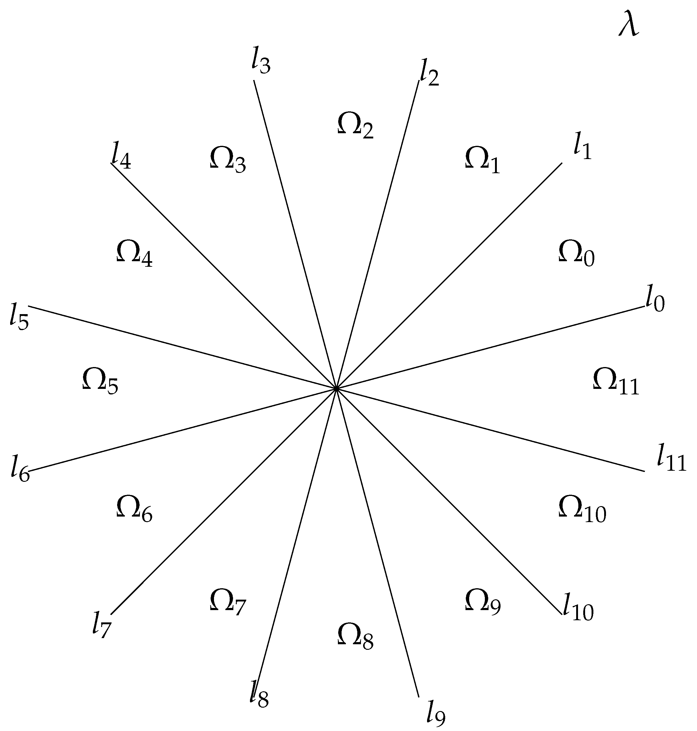
The continuous spectrum of L fills up the set of rays $l_{\nu }$, $\nu =0,\cdots 11$ in the complex $\lambda$-plane for which (see Figure 1)

$$\begin{array}{c}\hfill \mathrm{Im}{\lambda }^2\alpha \left(J\right)=0,\end{array}$$

(27)

where $\alpha$ is any root of $A_2$ where $\alpha \left(J\right)=\left(\alpha ,\overrightarrow{j}\right)$, with ${\left(\overrightarrow{j}\right)}_i=J_{ii}$ and $(,)$ denoting the standard scalar product. Solving (27) leads to the rays being defined by

$$\begin{array}{c}\hfill l_{\nu }=arg\lambda =\frac{\pi (\nu +\frac{1}{2})}{6},\nu =0,\cdots 11.\end{array}$$

(28)

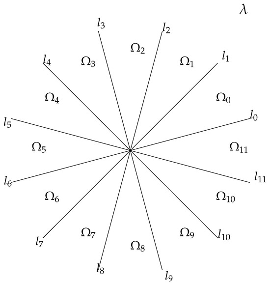Figure 1. The continuous spectrum of L fills up the rays $l_{\nu }$, $\nu =0,\cdots ,11$. Here, ${\mathrm{\Omega }}_{\nu }$ denotes the sectors of analyticity of the FAS ${\xi }_{\nu }(x,t,\lambda )$.

Each ray is related to a subalgebra ${\mathfrak{g}}_{\nu }$ with root systems ${\delta }_{\nu }$ whose roots satisfy

$$\begin{array}{c}\hfill {\delta }_{\nu }\equiv \{\alpha \in {\delta }_{\nu }\iff \mathrm{I}\mathrm{m}{\lambda }^2\alpha \left(J\right)=0,\forall \lambda \in l_{\nu }\}.\end{array}$$

(29)

More specifically, for this particular case we have

$$\begin{array}{cc}\hfill {\delta }_0& \equiv \{\pm (e_1-e_3)\},\hfill \\ \hfill {\delta }_1& \equiv \{\pm (e_1-e_2)\},\hfill \\ \hfill {\delta }_2& \equiv \{\pm (e_2-e_3)\},\hfill \end{array}$$

(30)

and ${\delta }_{\nu +3}\equiv {\delta }_{\nu }$.

2.

The regions of analyticity of the FAS ${\xi }_{\nu }(x,t,\lambda )$ are the sectors

$$\begin{array}{c}\hfill {\mathrm{\Omega }}_{\nu }\equiv \left\{\frac{\pi (\nu +\frac{1}{2})}{6}\le arg\lambda \le \frac{\pi (\nu +1+\frac{1}{2})}{6}\right\}.\end{array}$$

(31)

The FAS are introduced as the solutions of the following set of integral equations (written component-wise)

$$\begin{array}{c}\hfill {\xi }_{\nu ,jk}(x,t,\lambda )={\delta }_{jk}+i{\int }_{s_{jk}\infty }^{x}dy{e}^{-i{\lambda }^2(J_{jj}-J_{kk})(x-y)}{\left((U_0(y,t)+\lambda U_1(y,t)){\xi }_{\nu }(y,t,\lambda )\right)}_{jk},\end{array}$$

(32)

where $\lambda \in {\mathrm{\Omega }}_{\nu }$ and $s_{jk}$ take the values $\pm 1$, which are specific for each of the sectors ${\mathrm{\Omega }}_{\nu }$, see Table 1.

Table 1. The signs $s_{jk}$ in (32). The table contains the values of $s_{jk}$ for $j<k$ because $s_{kj}=-s_{jk}$. Also, the signs for ${\mathrm{\Omega }}_{\nu +3}$ and ${\mathrm{\Omega }}_{\nu +9}$ are opposite to the signs for ${\mathrm{\Omega }}_{\nu }$, $\nu =0,\cdots ,2$, while the signs for ${\mathrm{\Omega }}_{\nu +6}$ are the same. The signs are chosen in a way that ensures that the integral Equation (32) is correctly defined.

	$(1,2)$	$(1,3)$	$(2,3)$
${\mathrm{\Omega }}_0$	−	+	+
${\mathrm{\Omega }}_1$	+	+	+
${\mathrm{\Omega }}_2$	+	+	−

3.

In each sector ${\mathrm{\Omega }}_{\nu }$, the roots are ordered as follows: the root $\alpha$ is called $\nu$-positive (resp. $\nu$-negative) if $\mathrm{I}\mathrm{m}{\lambda }^2\alpha \left(J\right)>0$ (resp. $\mathrm{I}\mathrm{m}{\lambda }^2\alpha \left(J\right)<0$) for $\lambda \in {\mathrm{\Omega }}_{\nu }$. For example, the sets of positive roots of the subalgebras ${\mathfrak{g}}_{\nu }$ are

$$\begin{array}{cc}\hfill {\delta }_0^{+}& \equiv \left\{(e_1-e_3)\right\},\hfill \\ \hfill {\delta }_1^{+}& \equiv \left\{(e_1-e_2)\right\},\hfill \\ \hfill {\delta }_2^{+}& \equiv \{-(e_2-e_3)\}.\hfill \end{array}$$

(33)

Note that the root systems ${\delta }_{\nu }$ are isomorphic to the root system of $sl\left(2\right)$.

4.

The scattering data is obtained by the limits of the FAS along both sides of the rays $l_{\nu }{e}^{\pm i0}$:

$$\begin{array}{cc}\hfill \underset{x\to -\infty }{lim}{e}^{-i{\lambda }^{2}Jx}{\xi }_{\nu }(x,t,\lambda )e^{i{\lambda }^{2}Jx}& =S_{\nu }^{+}(t,\lambda ),\hfill \\ \hfill \underset{x\to \infty }{lim}{e}^{-i{\lambda }^{2}Jx}{\xi }_{\nu }(x,t,\lambda )e^{i{\lambda }^{2}Jx}& =T_{\nu }^{-}(t,\lambda )D_{\nu }^{+}\left(\lambda \right),\hfill \end{array}\forall \lambda \in l_{\nu }{e}^{+i0},$$

(34)

$$\begin{array}{cc}\hfill \underset{x\to -\infty }{lim}{e}^{-i{\lambda }^{2}Jx}{\xi }_{\nu }(x,t,\lambda )e^{i{\lambda }^{2}Jx}& =S_{\nu +1}^{-}(t,\lambda ),\hfill \\ \hfill \underset{x\to \infty }{lim}{e}^{-i{\lambda }^{2}Jx}{\xi }_{\nu }(x,t,\lambda )e^{i{\lambda }^{2}Jx}& =T_{\nu +1}^{+}(t,\lambda )D_{\nu +1}^{-}\left(\lambda \right),\hfill \end{array}\forall \lambda \in l_{\nu +1}{e}^{-i0},$$

(35)

where $S_{\nu }^{\pm }$, $T_{\nu }^{\pm }$ and $D_{\nu }^{\pm }$ are elements of the subgroup ${\mathcal{G}}_{\nu }$ (corresponding to the algebra ${\mathfrak{g}}_{\nu }$) of the form

$$\begin{array}{cc}\hfill S_{\nu }^{\pm }(t,\lambda )& =exp\left(\sum _{\alpha \in {\delta }_{\nu }^{+}}^{}{s}_{\alpha ,\nu }^{\pm }(t,\lambda )E_{\pm \alpha }\right),\hfill \\ \hfill T_{\nu }^{\pm }(t,\lambda )& =exp\left(\sum _{\alpha \in {\delta }_{\nu }^{+}}^{}{\tau }_{\alpha ,\nu }^{\pm }(t,\lambda )E_{\pm \alpha }\right),\hfill \\ \hfill D_{\nu }^{\pm }\left(\lambda \right)& =exp\left(\sum _{\alpha \in {\delta }_{\nu }^{+}}^{}{d}_{\alpha ,\nu }^{\pm }\left(\lambda \right)H_{\alpha }\right),\hfill \end{array}$$

(36)

satisfying

$$T_{\nu }^{-}{D}_{\nu }^{+}\widehat{S_{\nu }^{+}}=T_{\nu }^{+}{D}_{\nu }^{-}\widehat{S_{\nu }^{-}}=T_{\nu }(t,\lambda ),\lambda \in l_{\nu }.$$

(37)

Equation (37) is the Gauss decomposition of the scattering matrix $T_{\nu }(t,\lambda )$. Note that the functions $D_{\nu }^{+}$ and $D_{\nu +1}^{-}$ are analytic in the sector ${\mathrm{\Omega }}_{\nu }$.

5.

It can be shown, that the fundamental analytic solutions ${\xi }_{\nu }(x,t,\lambda )$ satisfy a (multiplicative) Riemann–Hilbert problem (RHP):

$$\begin{array}{cc}\hfill {\xi }_{\nu +1}(x,t,\lambda )& ={\xi }_{\nu }(x,t,\lambda )G_{\nu }(x,t,\lambda ),\hfill \\ \hfill G_{\nu }(x,t,\lambda )& =e^{i{\lambda }^{2}Jx}{\widehat{S}}_{\nu +1}^{-}(t,\lambda )S_{\nu +1}^{+}(t,\lambda )e^{-i{\lambda }^{2}Jx},\hfill \end{array}$$

(38)

which allows canonical normalization:

$$\underset{\lambda \to \infty }{lim}{\xi }_{\nu }(x,t,\lambda )=11.$$

(39)

It follows from the generalization of Zakharov–Shabat theorem for an L operator, quadratic in the spectral parameter [18], that the solution of the RHP (38) with canonical normalization is an FAS of the system

$$i\frac{\partial {\xi }_{\nu }}{\partial x}+(U_0+\lambda U_1){\xi }_{\nu }(x,t,\lambda )-{\lambda }^2[J,{\xi }_{\nu }(x,t,\lambda )]=0,$$

(40)

To make this more precise, since ${\xi }_{\nu }(x,t,\lambda )$ is canonically normalized, it has an asymptotic form given by

$$\begin{array}{c}\hfill {\xi }_{\nu }(x,t,\lambda )=exp\left(\mathcal{Q}(x,t,\lambda )\right),\end{array}$$

(41)

where, in general,

$$\begin{array}{c}\hfill \mathcal{Q}(x,t,\lambda )=\sum _{s=1}^{\infty }{\lambda }^{-s}{Q}_s(x,t).\end{array}$$

(42)

Following the idea of Gel’fand and Dikii [23], it can be shown [18] that for quadratic Lax operators only the first two terms are needed

$$\mathcal{Q}(x,t,\lambda )=\frac{Q_1(x,t)}{\lambda }+\frac{Q_2(x,t)}{{\lambda }^2}+....$$

(43)

with higher terms expressed as functions of $Q_1(x,t)$ and $Q_2(x,t)$ and their derivatives. Then, the potentials of L can be expressed as

$$\begin{array}{cc}\hfill U_1& ={\mathrm{ad}}_J{Q}_1,\hfill \\ \hfill U_0& ={\mathrm{ad}}_J{Q}_2-\frac{1}{2}{\mathrm{ad}}_{Q_1}^{2}J.\hfill \end{array}$$

(44)

The above can be inverted, allowing us to express $Q_1(x,t)$ and $Q_2(x,t)$ in terms of the potentials

$$\begin{array}{cc}\hfill Q_1& ={\mathrm{a}\mathrm{d}}_J^{-1}{U}_1,\hfill \\ \hfill Q_2& ={\mathrm{a}\mathrm{d}}_J^{-1}\left(U_0-\frac{1}{2}\left[U_1,{\mathrm{a}\mathrm{d}}_J^{-1}{U}_1\right]\right),\hfill \end{array}$$

(45)

which shows that ${\xi }_{\nu }(x,t,\lambda )$ is a solution of (40). Then, the FAS of the Lax operator L is given by ${\chi }_{\nu }(x,t,\lambda )={\xi }_{\nu }(x,t,\lambda )e^{i{\lambda }^{2}Jx}$.

Note that some of the scattering data defined above is redundant; i.e., there is a minimal set of scattering data. In fact, it can be shown that this set is determined entirely by the functions $S_{\nu }^{\pm }(t,\lambda )$.

Theorem 1. 

Let the solutions ${\xi }_{\nu }(x,t,\lambda )$ of the RHP (38) be regular; that is they have no zeros or singularities in their regions of analyticity. Then, a minimal set of scattering data that uniquely determines the scattering matrices $T_{\nu }(t,\lambda )$ and the potentials $U_0(x,t),U_1(x,t)$ is given by

$$\mathcal{T}\equiv \{s_{0,\alpha }^{+}(t,\lambda ),\alpha \in {\delta }_0^{+},s_{1,\alpha }^{\pm }(t,\lambda ),\alpha \in {\delta }_1^{+},s_{2,\alpha }^{\pm }(t,\lambda ),\alpha \in {\delta }_2^{+},s_{3,\alpha }^{-}(t,\lambda ),\alpha \in {\delta }_3^{-}\}.$$

(46)

Proof. 

The proof consists of four steps:

• Looking at the first equation from (36), the set of scattering data $\mathcal{T}$ uniquely determines the matrices $S_1^{\pm }(t,\lambda )$ for $\lambda \in l_1{e}^{\pm i0}$, $S_2^{\pm }(t,\lambda )$ for $\lambda \in l_2{e}^{\pm i0}$ and $S_3^{\pm }(t,\lambda )$ for $\lambda \in l_3{e}^{\pm i0}$. The Coxeter reduction implies that

  $$\begin{array}{cc}\hfill S_{3\nu }^{\pm }(t,\lambda )& =c^{\nu }{S}_0^{\pm }(t,{\omega }^{-\nu }\lambda )c^{-\nu },\lambda \in l_{\nu }{e}^{\pm i0},\hfill \\ \hfill S_{3\nu +1}^{\pm }(t,\lambda )& =c^{\nu }{S}_1^{\pm }(t,{\omega }^{-\nu }\lambda )c^{-\nu },\lambda \in l_{\nu +1}{e}^{\pm i0},\hfill \\ \hfill S_{3\nu +2}^{\pm }(t,\lambda )& =c^{\nu }{S}_2^{\pm }(t,{\omega }^{-\nu }\lambda )c^{-\nu },\lambda \in l_{\nu +2}{e}^{\pm i0}.\hfill \end{array}$$

  (47)
  This determines $S_{\nu }^{\pm }\left(\lambda \right)$ on the rest of the rays.
• $D_{\nu }^{\pm }\left(\lambda \right)$ are determined uniquely by $S_{\nu }^{\pm }(t,\lambda )$. The regularity of ${\xi }_{\nu }(x,t,\lambda )$ implies that the functions $D_{\nu }^{\pm }\left(\lambda \right)$ are also regular, i.e., have no zeros or singularities. This also means that the functions $d_{\alpha ,\nu }^{\pm }\left(\lambda \right)$ from the last equation in (36) are analytical. We will use the regularity of $D_{\nu }^{\pm }\left(\lambda \right)$ along with (37). In what follows, the reader is assumed to have some familiarity with the representation theory of simple Lie algebras.
  Let ${\omega }_{\nu ,j}^{+}$ be the j-th fundamental weight of the subalgebra ${\mathfrak{g}}_{\nu }$ evaluated (with respect to the index j) with the ordering in ${\mathrm{\Omega }}_{\nu }$. Let $|{\omega }_{\nu ,j}^{\pm }⟩$ (here, we are using standard Bra–ket notation) be the corresponding weight vector in the fundamental representation of ${\mathfrak{g}}_{\nu }$ that has highest weight ${\omega }_{\nu ,j}^{+}$ (respectively, ${\omega }_{\nu ,j}^{-}$ is the lowest weight). Then, considering that for all $\alpha \in {\delta }_{\nu }^{+}$

  $$E_{\alpha }|{\omega }_{\nu ,j}^{+}⟩=0,E_{-\alpha }|{\omega }_{\nu ,j}^{-}⟩=0,⟨{\omega }_{\nu ,j}^{+}|E_{-\alpha }=0,⟨{\omega }_{\nu ,j}^{-}|E_{\alpha }=0,$$

  (48)

  we have

  $$\begin{array}{cccc}\hfill ⟨{\omega }_{\nu ,j}^{+}|S_{\nu }^{-}& =⟨{\omega }_{\nu ,j}^{+}|T_{\nu }^{-}=⟨{\omega }_{\nu ,j}^{+}|,\hfill & \hfill ⟨{\omega }_{\nu ,j}^{-}|S_{\nu }^{+}& =⟨{\omega }_{\nu ,j}^{-}|T_{\nu }^{+}=⟨{\omega }_{\nu ,j}^{-}|,\hfill \\ \hfill S_{\nu }^{+}|{\omega }_{\nu ,j}^{+}⟩& =T_{\nu }^{+}|{\omega }_{\nu ,j}^{+}⟩=|{\omega }_{\nu ,j}^{+}⟩,\hfill & \hfill S_{\nu }^{-}|{\omega }_{\nu ,j}^{-}⟩& =T_{\nu }^{-}|{\omega }_{\nu ,j}^{-}⟩=|{\omega }_{\nu ,j}^{-}⟩\hfill \end{array}$$

  (49)

  and

  $$\begin{array}{cc}\hfill D_{\nu }^{+}|{\omega }_{\nu ,j}^{+}⟩& =e^{d_{{\alpha }_j,\nu }^{+}}|{\omega }_{\nu ,j}^{+}⟩,D_{\nu }^{-}|{\omega }_{\nu ,j}^{-}⟩=e^{-d_{{\alpha }_j,\nu }^{-}}|{\omega }_{\nu ,j}^{-}⟩.\hfill \end{array}$$

  (50)
  Analogous relations can also be derived for the inverses. Note that we can rewrite (37) in the form of

  $$\begin{array}{c}\hfill D_{\nu }^{-}\widehat{S_{\nu }^{-}}{S}_{\nu }^{+}{\widehat{D}}_{\nu }^{+}={\widehat{T}}_{\nu }^{+}{T}_{\nu }^{-},\lambda \in l_{\nu }.\end{array}$$

  (51)
  Then, by squeezing (51) between $⟨{\omega }_{\nu ,j}^{\pm }|\dots |{\omega }_{\nu ,j}^{\pm }⟩$ we obtain that

  $$\begin{array}{cc}\hfill d_{{\alpha }_j,\nu }^{+}-d_{{\alpha }_j,\nu }^{-}& =ln⟨{\omega }_{\nu ,j}^{-}\left|{\widehat{S}}_{\nu }^{-}{S}_{\nu }^{+}\right|{\omega }_{\nu ,j}^{-}⟩\hfill \\ \hfill & =-ln⟨{\omega }_{\nu ,j}^{+}\left|{\widehat{T}}_{\nu }^{+}{T}_{\nu }^{-}\right|{\omega }_{\nu ,j}^{+}⟩.\hfill \end{array}$$

  (52)
  The functions $d_{{\alpha }_j,\nu }^{\pm }$ can be recovered uniquely from their analyticity properties and from the jumps (52) along the rays $l_{\nu }$. This in turn determines $D_{\nu }^{\pm }\left(\lambda \right)$. The exact details are essentially the same as for linear Lax operators and can be found in [16]).
• The matrices $T_{\nu }^{\pm }(t,\lambda )$ are recovered as the Gauss factors of the right hand side of (51).
• Finally, the corresponding potentials are reconstructed from the regular solutions of the RHP (38) by taking the limit $\lambda \to \infty$ in

  $$\begin{array}{c}\hfill \left(\frac{\partial {\xi }_{\nu }}{\partial x}(x,t,\lambda )\right){\widehat{\xi }}_{\nu }(x,t,\lambda )+U_0(x,t)+\lambda U_1(x,t)={\lambda }^2\left(J-{\xi }_{\nu }(x,t,\lambda )J{\widehat{\xi }}_{\nu }(x,t,\lambda )\right).\end{array}$$

  (53)

□

6. Time Dependence of the Scattering Data

The ZCR ensures that the operators L and M have the same set of FAS. In general, we have that

$$L{\chi }_{\nu }(x,t,\lambda )=0,M{\chi }_{\nu }(x,t,\lambda )-{\chi }_{\nu }(x,t,\lambda )\mathrm{\Gamma }\left(\lambda \right)=0,$$

(54)

with ${\chi }_{\nu }(x,t,\lambda )={\xi }_{\nu }(x,t,\lambda )e^{i{\lambda }^{2}Jx}$ and $\mathrm{\Gamma }\left(\lambda \right)$ is a constant matrix. The idea is to choose $\mathrm{\Gamma }\left(\lambda \right)$ in such a way so that the scattering data satisfy a linear evolution equation.

Assuming $\lambda \in l_{\nu }{e}^{i0}$, let us calculate the following limit:

$$\begin{array}{cc}\hfill & \underset{x\to -\infty }{lim}{e}^{-i{\lambda }^{2}Jx}M{\chi }_{\nu }(x,t,\lambda )=\hfill \\ \hfill & =\underset{x\to -\infty }{lim}{e}^{-i{\lambda }^{2}Jx}\left[\left(i\frac{\partial }{\partial t}+\sum _{p=0}^4{\lambda }^p{V}_p-{\lambda }^{4}K\right){\chi }_{\nu }(x,t,\lambda )-{\chi }_{\nu }(x,t,\lambda )\mathrm{\Gamma }\left(\lambda \right)\right]\hfill \\ \hfill & =i\frac{\partial S_{\nu }^{+}}{\partial t}-{\lambda }^{4}K{S}_{\nu }^{+}(t,\lambda )-S_{\nu }^{+}(t,\lambda )\mathrm{\Gamma }\left(\lambda \right)=0,\lambda \in l_{\nu }{e}^{+i0},\hfill \end{array}$$

(55)

where we have used the fact that ${lim}_{x\to \pm \infty }{V}_k(x,t)=0$. From the diagonal part of (55), considering that from (36) it follows that $S_{\nu }^{+}(t,\lambda )$ are unitriangular matrices, and we obtain

$$\begin{array}{c}\hfill {\lambda }^{4}K+\mathrm{\Gamma }\left(\lambda \right)=0,\end{array}$$

(56)

which means that $\mathrm{\Gamma }\left(\lambda \right)=-{\lambda }^{4}K$. Then, the last line of (55) becomes

$$i\frac{\partial S_{\nu }^{+}}{\partial t}-{\lambda }^4[K,S_{\nu }^{+}(t,\lambda )]=0,\lambda \in l_{\nu }{e}^{+i0}.$$

(57)

A similar limit can be calculated for $x\to \infty$:

$$\begin{array}{cc}\hfill & \underset{x\to \infty }{lim}{e}^{-i{\lambda }^{2}Jx}M{\chi }_{\nu }(x,t,\lambda )=\hfill \\ \hfill & =\underset{x\to \infty }{lim}{e}^{-i{\lambda }^{2}Jx}\left[\left(i\frac{\partial }{\partial t}+\sum _{p=0}^4{\lambda }^p{V}_p-{\lambda }^{4}K\right){\chi }_{\nu }(x,t,\lambda )-{\chi }_{\nu }(x,t,\lambda )\mathrm{\Gamma }\left(\lambda \right)\right]\hfill \\ \hfill & =i\frac{\partial T_{\nu }^{-}{D}_{\nu }^{+}}{\partial t}-{\lambda }^4[K,T_{\nu }^{-}(t,\lambda )D_{\nu }^{+}\left(\lambda \right)]=0.\hfill \end{array}$$

(58)

Again, considering the diagonal part and (36), we have

$$\begin{array}{c}\hfill i\frac{\partial D_{\nu }^{+}}{\partial t}=0,\end{array}$$

(59)

i.e., the matrix elements of $D_{\nu }^{+}\left(\lambda \right)$ are generating functionals of the integrals of motion of the corresponding system of dNLS-type equations.

Note that we could have used as a minimal set of scattering data the functions $T_{\nu }^{\pm }(t,\lambda )$ —they form an equivalent set. We can derive a similiar evolution for $T_{\nu }^{\pm }(t,\lambda )$ by considering the lower triangular part of (58)

$$i\frac{\partial T_{\nu }^{-}}{\partial t}-{\lambda }^4[K,T_{\nu }^{-}(t,\lambda )]=0,\lambda \in l_{\nu }{e}^{+i0}.$$

(60)

Doing an analogous procedure for $\lambda \in l_{\nu }{e}^{-i0}$ and evaluating the limits for $x\to \pm \infty$ results in

$$\begin{array}{cccc}\hfill i\frac{\partial S_{\nu }^{+}}{\partial t}& -{\lambda }^4[K,S_{\nu }^{+}(t,\lambda )]=0,\hfill & \hfill i\frac{\partial T_{\nu }^{-}}{\partial t}& -{\lambda }^4[K,T_{\nu }^{-}(t,\lambda )]=0,\lambda \in l_{\nu }{e}^{+i0},\hfill \\ \hfill i\frac{\partial S_{\nu }^{-}}{\partial t}& -{\lambda }^4[K,S_{\nu }^{-}(t,\lambda )]=0,\hfill & \hfill i\frac{\partial T_{\nu }^{+}}{\partial t}& -{\lambda }^4[K,T_{\nu }^{+}(t,\lambda )]=0,\lambda \in l_{\nu }{e}^{-i0}\hfill \end{array}$$

(61)

with the diagonal factors $D_{\nu }^{\pm }\left(\lambda \right)$ being t-independent.

The solution of the above equations is given by (written component-wise)

$$S_{\nu ,jk}^{\pm }(t,\lambda )=e^{i{\lambda }^4(K_j-K_k)t}{S}_{\nu ,jk}^{\pm }(0,\lambda ),T_{\nu ,jk}^{\pm }(t,\lambda )=e^{i{\lambda }^4(K_j-K_k)t}{T}_{\nu ,jk}^{\pm }(0,\lambda ).$$

(62)

Solving the corresponding system of a non-linear evolution equation (NLEE) reduces to solving the direct and the inverse scattering problem for the Lax operator L.

7. Concluding Remarks

When dealing with exactly solvable non-linear models, there are two points to consider. The first is the purely mathematical interest in the subject. In that regard, the results of this paper will mainly be of interest to specialists in exactly solvable non-linear models, especially soliton theory, as the derived equation form a system of PDE’s which possess soliton solutions. The other aspect is the practical application. The truth is that only a small number of all known exactly solvable non-linear models have found application in practice—KdV, NLS, dNLS, etc. However, this does not mean that there is no value in finding generalizations—for example, the Manakov model is a multi-component generalization of the NLS equation, and it finds applications in optics. In general, one cannot know a priori which exactly solvable model will find application in a given practical context. The best strategy, then, is to create a list of all possible exactly solvable models. Considering 1 + 1 variables, for L linear in $\lambda$, this list seems to be almost exhausted (at least for practical number of components). What is left is either to consider polynomial dependence on $\lambda$ or some entirely new approach not based on the Lax representation. The article considers the first possibility and focuses on Lax operators related to Kac–Moody algebras.

There are, however, some details that need further study:

• The first is a rigorous study of the mapping between potential $(U_0,U_1)$ and scattering matrix $T_{\nu }$. In defining the FAS, we assumed that Equation (32) has a solution which is obviously not true for all classes of potentials (it is true for potentials on compact support and for Schwartz functions). The first step is a mathematically rigorous definition of the class of admissible potentials, such that the mapping $(U_0,U_1)\mapsto T_{\nu }$ and its inverse are correctly defined. This problem in the case of linear L operators [16,17,23] is rather involved and the same is expected to be true for the quadratic case.
• There is a hierarchy of integrable systems of equations related to a single L operator. This can be derived with the help of the recursion operators. Finding their explicit form is somewhat difficult. One can infer from the solution of the recursion relations, i.e., Equation (36), that for an L operator of order m in $\lambda$, the recursion operator will have m arguments (i.e., a tensor of rank $m+1$).
• The hierarchy of integrable equations admits a Hamiltonian formulation. Since the factors $D_{\nu }^{\pm }$ generate the integrals of motion for the system, they can be used to find the Hamiltonian. In the general case, the Hamiltonian can also be found by using the recursion operators [14].
• Finding the multi-soliton solutions of the corresponding equations. This can be done, for example, by using the dressing method, with the procedure being more involved for polynomial L operators [18].
• If the soliton solutions are found by the dressing method, then the soliton dynamics and interactions can be studied by considering the asymptotic behavior of the dressing factor.

The algebra $A_2^{\left(1\right)}$ was chosen since it is the simplest non-trivial case for which a system of exactly solvable NLEEs can be derived with a L operator quadratic in $\lambda$. The methods presented in this article can be used to derive other exactly solvable models, for example, by considering Lax pairs related to other Kac–Moody algebras.

References

- Gardner, C.S.; Greene, J.M.; Kruskal, M.D.; Miura, R.M. Method for solving the Korteweg-de Vries equation. Phys. Rev. Lett. 1967, 19, 1095–1097. [Google Scholar] [CrossRef]
- Lax, P.D. Integrals of nonlinear equations of evolution and solitary waves. Commun. Pure Appl. Math. 1968, 21, 467–490. [Google Scholar] [CrossRef]
- Zakharov, V.E.; Shabat, A.B. A scheme for integrating the nonlinear equations of mathematical physics by the method of the inverse scattering problem. I Funct. Anal. Appl. 1974, 8, 226–235. [Google Scholar] [CrossRef]
- Zakharov, V.E.; Shabat, A.B. Integration of nonlinear equations of mathematical physics by the method of inverse scattering. II. Funct. Anal. Appl. 1979, 13, 166–174. [Google Scholar] [CrossRef]
- Manakov, S.V. On the theory of two-dimensional stationary self-focusing of electromagnetic waves. Sov. Phys. JETP 1974, 38, 248–253. [Google Scholar]
- Kaup, D.J.; Newell, A.C. An exact solution for a derivative nonlinear Schrödinger equation. J. Math. Phys. 1978, 19, 798–801. [Google Scholar] [CrossRef]
- Chen, H.H.; Lee, Y.C.; Liu, C.S. Integrability of Nonlinear Hamiltonian Systems by Inverse Scattering Method. Phys. Scr. 1979, 20, 490. [Google Scholar] [CrossRef]
- Gerdjikov, V.S.; Ivanov, M.I. The quadratic bundle of general form and the nonlinear evolution equations: Expansions over the “squared” solutions-generalized Fourier transform. Bulg. J. Phys. 1983, 10, 130. [Google Scholar]
- Mikhailov, A.V. The reduction problem and the inverse scattering method. Phys. Nonlinear Phenom. 1981, 3, 73–117. [Google Scholar] [CrossRef]
- Gerdjikov, V.S. Derivative Nonlinear Schrödinger Equations with ZN and DN–Reductions. Rom. J. Phys. 2013, 58, 573–582. [Google Scholar]
- Drinfeld, V.G.; Sokolov, V.V. Equations of KdV type and simple Lie algebras. Sov. Math. Dokl. 1981, 23, 457–462. [Google Scholar]
- Drinfel’d, V.G.; Sokolov, V.V. Lie algebras and equations of Korteweg-de Vries type. Sov. J. Math. 1985, 30, 1975–2036. [Google Scholar] [CrossRef]
- Gerdjikov, V.S.; Mladenov, D.M.; Stefanov, A.A.; Varbev, S.K. Integrable equations and recursion operators related to the affine Lie algebras . J. Math. Phys. 2015, 56, 052702. [Google Scholar] [CrossRef]
- Gerdjikov, V.S.; Stefanov, A.A.; Iliev, I.D.; Boyadjiev, G.P.; Smirnov, A.O.; Matveev, V.B.; Pavlov, M.V. Recursion operators and hierarchies of mKdV equations related to the Kac–Moody algebras , , and . Theor. Math. Phys. 2020, 204, 1110–1129. [Google Scholar] [CrossRef]
- Beals, R.; Coifman, R.R. Scattering and inverse scattering for first order systems. Commun. Pure Appl. Math. 1984, 37, 39–90. [Google Scholar] [CrossRef]
- Gerdjikov, V.S.; Yanovski, A.B. Completeness of the eigenfunctions for the Caudrey-Beals-Coifman system. J. Math. Phys. 1994, 35, 3687–3725. [Google Scholar] [CrossRef]
- Gerdjikov, V.S.; Yanovski, A.B. CBC systems with Mikhailov reductions by Coxeter Automorphism: I. Spectral Theory of the Recursion Operators. Stud. Appl. Math. 2015, 134, 145–180. [Google Scholar] [CrossRef]
- Gerdjikov, V.S.; Stefanov, A.A. Riemann-Hilbert problems, polynomial Lax pairs, integrable equations and their soliton solutions. Symmetry 2023, 15, 1933. [Google Scholar] [CrossRef]
- Krishnaswami, G.S.; Vishnu, T.R. An introduction to Lax pairs and the zero curvature representation. arXiv 2020, arXiv:2004.05791v1. [Google Scholar]
- Carter, R. Lie Algebras of Finite and Affine Type; Cambridge University Press: Cambridge, UK, 2005. [Google Scholar]
- Kac, V. Infinite Dimensional Lie Algebras; Cambridge University Press: Cambridge, UK, 1995. [Google Scholar]
- Helgasson, S. Differential Geometry, Lie Groups and Symmetric Spaces; Graduate Studies in Mathematics 34; AMS: Providence, RI, USA, 2012. [Google Scholar]
- Gel’fand, I.M.; Dikii, L.A. The calculus of jets and nonlinear Hamiltonian systems. Funct. Anal. Appl. 1978, 12, 81–94. [Google Scholar] [CrossRef]
Disclaimer/Publisher’s Note: The statements, opinions and data contained in all publications are solely those of the individual author(s) and contributor(s) and not of MDPI and/or the editor(s). MDPI and/or the editor(s) disclaim responsibility for any injury to people or property resulting from any ideas, methods, instructions or products referred to in the content. |
© 2024 by the author. Licensee MDPI, Basel, Switzerland. This article is an open access article distributed under the terms and conditions of the Creative Commons Attribution (CC BY) license (https://creativecommons.org/licenses/by/4.0/).