Abstract
This work is an attempt to modernise Weber’s electrodynamics to make it compatible with the high-velocity regime, and with the existence of a limiting velocity, c. For this purpose, starting from the law of energy conservation and the mass–energy equivalence, new expressions for potential energy and for kinetic energy are derived jointly which are consistent with an ultimate velocity of the value of c. The new potential energy, already reported by Phipps, becomes Weber’s expression in the limit of low velocities. The new kinetic energy differs from the relativistic expression, but, like the latter, it also becomes the Newtonian expression in the limit of low velocities. New expressions for force and linear momentum are also derived which complete a new mechanics. Phipps’ potential energy and new kinetic energy are applied to the problem of two interacting charges in a radial motion and orbital motion. The new framework is also applied to the problem of a charge moving between the two plates of a charged capacitor, obtaining a result similar to that obtained by means of Maxwell–Lorentz electromagnetism and relativistic mechanics. The metaphysical considerations that clearly differentiate the conventional framework from the new framework proposed here are discussed.
1. Introduction
Probably, one of the most interesting questions in fundamental physics is how two electric charges interact when they are in relative motion. This subject was able to capture the attention of the most brilliant minds of the 19th and 20th centuries. At the beginning of the 19th century, Ampère [1], Gauss [2], Weber [3] and Riemann [4] (highly influential figures in science at that time) developed different electrodynamic theories extending the well-known Coulomb’s law. These were laws of instantaneous action-at-a-distance, in which the concept of “field” was completely absent. In this context, Weber developed his electrodynamic theory during the same period in which Maxwell was working on his equations. Maxwell, though he was a strong advocate of the field idea, studied Weber’s theory rigorously, praised it repeatedly, and analysed it in detail in the last chapter of his most famous work Treatise [5], considering it a promising alternative approach to his own.
Despite being in line with the most commonly recognised facts of electromagnetism and Maxwell’s endorsement, Weber’s electrodynamics gradually fell into oblivion. Today, Weber’s name only appears in textbooks in connection with the unit of magnetic flux in the International System of Units, as the only recognition of his research prowess. One of the reasons for this neglect, perhaps the main one, is that Weber’s theory was unable to predict the propagation of electromagnetic waves in a vacuum, as Maxwell’s theory was able to do. Interestingly, Weber and Kirchhoff had been the first to show that the electrical signal should travel through conducting wires in the form of travelling waves with velocity, c. However, the reasoning employed there was not valid in a vacuum, where there were no supporting electric charges. Another reason that undermined confidence in Weber’s electrodynamics was Helmholtz’s fierce criticism, arguing that the theory involved a violation of the law of energy conservation and predicted that, under certain configurations, charges could act as if they had a negative inertial mass, contrary to experiments. Weber vigorously refuted the first criticism in [6], and Maxwell, in his study of Weber’s electrodynamics, ruled that Weber’s electrodynamics did satisfy the law of energy conservation [5]. However, the doubts and misgivings about the theory would never disappear. The advent of the special relativity theory (SRT), which rejects the absolute simultaneity of two distant events, dealt a mortal blow to the concept of action-at-a-distance and condemned as heretical all theories that relied on it. Interestingly, however, in recent years, the concept of action-at-a-distance has been making an increasingly strong comeback in the field of quantum physics [7,8].
Weber’s electrodynamics, like Gauss’s and Riemann’s, were expressed in terms of the interaction force between two charged particles in relative motion. However, unlike other theories, Weber’s force satisfies Newton’s law of action and reaction in its strongest form and, as such, is compatible with the conservation of linear and angular momentum. It can be derived from a generalised velocity-dependent potential energy and is compatible with the law of energy conservation. From it can be derived Coulomb’s law, Faraday’s law of induction and Ampère’s expression for the force between current elements.
The most detailed and rigorous current treatise on Weber’s electrodynamics is the one written by Assis [9]. A comprehensive review of the state of the art on this topic, including the most relevant and the most recent contributions, can be found in [10]. New and recent work extending the experimental verification of the predictions of Weber’s electrodynamic theory can be found in [11,12,13,14,15,16,17,18,19,20,21,22,23,24].
Weber’s potential energy equation can be written as [9].
In this expression, UW is the potential energy generated by q1 and q2, ε0 is the vacuum’s permittivity, c is the velocity of light in the vacuum, r is the distance separating the two charges, and the dot stands for the time derivation, , so represents the radial relative velocity. Notice that Equation (1) is fully relational; that is, it is dependent only on the two interacting charges, on the distance between them (r) and on their radial relative velocity ().
In order to overcome Helmholtz’s objection to Weber’s law (the ‘negative mass behaviour’ for all velocities of a value less than that of c), Phipps proposed [25] a new expression for electrodynamic potential energy:
It is obvious that both Equations (1) and (2) implicitly contemplate a radial relative velocity that we can call critical. In Weber’s expression, this critical velocity takes the value of , whereas in Phipps’ expression, it takes the value of c. From a strictly mathematical point of view, in Weber’s expression the value of needs not be a limiting value, so that higher values are conceivable (although the sign of the energy would change from attractive to repulsive or vice versa). In Phipps’ expression, on the other hand, the value of c is a full-fledged limiting value, because higher values would imply non-real (complex) quantities. This is a difference to be taken into account.
It is easy to show that Weber’s expression can be seen as an approximate version of Phipps’ expression, valid only for situations where (low velocities). It is sufficient to take Maclaurin’s development of Phipps’ expression, retaining only the terms up to second order in ; the expression thus obtained coincides exactly with the one proposed by Weber.
The forces deriving from the above potential energies can be found by taking into account that
where is the unit vector in the direction of , and the vector connecting the two charges: from q2 to q1.
Applying Equation (3) to Equations (1) and (2) gives the following expressions for the respective forces:
Note that, in both cases, these are central forces, always directed along the line joining the two interacting charges.
On the other hand, the central forces can also be calculated from the kinetic energy, by means of:
Thus, for the central forces, the total energy is conserved, i.e.,
as is easily inferred by taking into account Equations (3) and (6), according to which and . The conservation of energy is completely independent of the expression adopted for kinetic energy, provided that the latter is correctly defined.
Therefore, in the studies carried out by different authors using Weber’s or Phipps’ electrodynamic potential energy, the Newtonian expression of kinetic energy has been used, due to the confidence that the existence of a limiting velocity was already guaranteed by the expression of the potential energy. However, there seems to be sufficient evidence that this strategy is not sufficient to reproduce some experimental results involving high velocities, and to yield predictions consistent with those of SRT [26,27]. Therefore, some authors have tentatively used other expressions for kinetic energy, such as the one deduced by Schrödinger [28] or the well-known relativistic expression [29]. Some works in this direction are those conducted in [30,31], although the results obtained have not been considered fully satisfactory. The theoretical effort to renew the expression for kinetic energy did not accompany the modernising attempt that led to the introduction of Phipps’ expression. The tentative or heuristic search for the most convenient expression for kinetic energy to be used in conjunction with Phipps’ expression for potential energy could prove tedious and, in the end, lack convincing power. Interesting work in this direction can be found in [32]. However, it would be ideal to find a deductive procedure which, starting on a firm basis, would allow the simultaneous derivation of the expressions of potential and kinetic energies. The basis of our deduction could be the law of energy conservation and the mass–energy equivalence.
In this work, based on these principles and following a reasoning similar to that adopted by Wesley in [33] to derive Weber’s potential energy, we shall show that it is possible to deduce jointly the expression of Phipps’ potential energy and the expression of kinetic energy that is compatible with it.
From the new expression for kinetic energy, we will derive new expressions for (linear) momentum and force (fundamental law of dynamics) applicable to the study of the radial motion of two interacting charges. We will then extend the study to the orbital motion of these charges, proposing new expressions for kinetic energy, linear momentum, angular momentum and force. Finally, an attempt will be made to solve, in the new framework, the problem of a charge moving perpendicularly to the plates of a charged capacitor.
All the proposed expressions will be analysed to check whether or not in the limit of low velocities and low energy, they are reduced to the expressions known in Newtonian mechanics. The results obtained in the new framework will also be contrasted with the predictions obtained in the Maxwell–Lorentz and SRT framework, in particular, to check that c is a limiting velocity.
2. New Mechanics for New Electrodynamics
2.1. Derivation of Potential and Kinetic Energies
Considering two charges, q1 and q2, with respective masses m1 and m2, interacting with each other and isolated from the rest of the universe, both particles will, in general, move around their common centre of mass. To facilitate the calculations, we can adopt the reduced mass procedure. By this procedure, the two-particle problem is reduced to that of a single particle with charge q1 and mass (μ) calculated via
moving with respect to the other particle, of charge q2, which is in this case ‘fixed’, at a distance, r.
Supposing charge q1 starts to move and acquires kinetic energy (T), by virtue of the mass–energy equivalence, the inertial mass of the system should be increased by the value . If the initial energy of the system is E, then the total mass of the charge in motion should be , where is the Coulomb potential energy, which is given by
Assuming that the acting force, F, can be calculated as a derivative of the momentum with respect to time, i.e.,
as charge q1 moves away from the fixed q2 charge, the rate to increase its kinetic energy by, , will be equal to the rate at which the force does work on charge q1. Thus,
and from here
In order to simplify the latter expression, we define the function γ as
the derivative of which, with respect to time, gives
and here,
Then, by inserting the latter result in Equation (12) and manipulating it algebraically, we obtain
which we can rewrite as
Additionally, from here,
Integrating this first-order ordinary differential equation between the corresponding limits of integration:
the following is obtained:
Restricting it to the case where initial energy is only potential, then and , so that Equation (20) becomes
Equation (21) is the expression of the law of energy conservation, and it includes Coulomb’s potential energy and the well-known relativistic expression for kinetic energy.
Now dividing Equation (21) by γ, and adding E to the two members of the equality, we obtain
which we can regroup as
If, in view of this equation, we now define the new electrodynamic potential energy, U, and its corresponding kinetic energy, T, as
then
On the one hand, Equation (26) coincides with the expression for the electrodynamic potential energy proposed by Phipps, Equation (2). On the other hand, Equation (27) is the new expression for the kinetic energy compatible with Phipps’ potential energy. This expression differs from the relativistic expression and has a different upper bound. Indeed, if , then , instead of , which is the case with the relativistic expression. A further difference is that in Equation (27), to the intrinsic inertial energy, , the inertial contribution from the total energy of the system, E, must now be added, which is not the case in the relativistic expression.
2.2. Limit of Low Radial Velocities and Low Energies
In the limit of low radial velocities, from Equation (26), Weber’s potential energy expression is recovered:
Assuming further that , Equation (27) recovers the Newtonian expression for kinetic energy:
Thus, it can be concluded that it is consistent to use the Newtonian expression for kinetic energy together with Weber’s potential energy, but with Phipps’ potential energy, Equation (27) must be used, if the mass–energy equivalence is to be guaranteed.
2.3. Discussion
In the conventional approach, electrostatic potential energy (Coulomb’s law) does not depend on . The dependence on velocity only resides in kinetic energy, both in the classical (Newtonian) and relativistic (SRT) frameworks. Therefore, in the latter case, all the mathematics to prevent velocities from exceeding the limiting value of c must be contained in the kinetic energy expression. The solution provided by the SRT is that the kinetic energy increases with increasing velocity, tending to be infinity as the velocity approaches the value of c.
In Weber’s or Phipps’ electrodynamics, the situation is not the same, since both potential energy and kinetic energy depend on . This double dependence might seem an unnecessary complexity in view of the success of the alternative (Coulomb-based) approach, but it could be justified if it could explain the same known phenomena without having to accept the epistemologically harder points of SRT, such as time dilations and space contractions.
According to Equation (27), the maximum value of the kinetic energy is and not infinity, as is the case for relativistic kinetic energy. Particle accelerators may seem to be excellent proof that SRT is the correct choice. However, this is not the case. With Phipps’ electrodynamics, the potential energy tends to be zero as ; i.e., the force on the interacting particles tends to be zero as , so they can no longer gain energy. Our belief that particles travelling inside particle accelerators have very high energies is due to the proven difficulty of slowing them down. However, since any deceleration must be caused by an electromagnetic force, if these were of the Weberian type (such as Phipps’ force), they would be extraordinarily weak (and therefore be highly ineffective at slowing down) until the particles are travelling at speeds much slower than the speed of light. This ignored inefficiency of the forces to achieve deceleration would create the appearance that the particles actually had very high initial energy values. The mathematics of these two competing theoretical models are very different, but both are perfectly self-consistent.
In light of our demonstration, the energy balances of Equations (21) and (23) are mathematically equivalent, although metaphysically speaking they respond to very different approaches. However, we insist, only if Phipps’ electrodynamics (together with the new expression for kinetic energy) can explain the totality of known electromagnetic phenomena, its apparently greater complexity would be justified, because it would be achieved without the need to appeal to the space-time approaches of SRT.
3. The Two-Body Problem in the New Framework
3.1. Radial Motion
Supposing the system consisting of two charges (q1 and q2) and a reduced mass, μ, given by Equation (8), interacting with each other according to Phipps’ potential energy, Equation (26), and which are radially displaced relative to each other, according to the expression of the kinetic energy given by Equation (27), for this system, using the reduced mass procedure, the law of energy conservation will require that
which can be rewritten as
additionally simplifying
which turns out to be the same expression that would have been obtained using Coulomb’s potential energy and the relativistic kinetic energy.
Solving for , it follows that
where .
Except in those mathematical situations that revert to a complex (non-real) , is fulfilled, which is what would be expected according to SRT. However, if we analyse the interaction between two charges of the same mass, with velocities and with respect to a reference frame bound to the centre of mass, we obtain , and not , as would be expected from SRT [34]. With Weber’s and Phipps’ electrodynamics (see [26,35,36,37]), it is not possible to obtain, simultaneously, and .
The price to pay for accepting the reorganisation implied by the definitions contained in Equations (24) and (25) is that, in addition to adopting a new expression for kinetic energy, we must also modify the expressions for force and momentum. The new expression for kinetic energy, given by Equation (27), requires an expression for force that is different from the Newtonian one (). We can find it simply by appealing to the definition of Equation (6):
An expression for the kinetic energy similar to that described by Equation (27) was already reported by Li in [32], where it was derived from a postulated expression for the force, which is equal to that of Equation (34). In contrast, in this work, Equation (34) has not been postulated, but has been derived from the kinetic energy expression, which is also not postulated, but deduced from the mass–energy equivalence.
Additionally, the expression of momentum, , will have to change. Keeping the definition as essential, then , so that, taking into account Equation (34), it follows that
which when integrated turns out to be
A similar expression was also reported by Li in [32]. Note that when , and that when . Note, also, that since the definition is preserved, then Newton’s third law of action and reaction is also satisfied in an isolated system with no external forces acting on it (momentum is conserved).
In the limit of low radial velocities and low energies (), Equation (34), referring to the force, can be simplified to
which is the well-known expression of Newton’s second law.
In the same limit again, from Equation (36), referring to the momentum, the Newtonian expression will also be recovered:
The dynamic analysis of the motion is achieved by equating the expression of Phipps’ force, given by Equation (5), with the new expression of the second law of dynamics, Equation (34). The result is greatly simplified and leads to
It can be seen that in the low-energy limit (), this expression is similar, except for a factor of ½ in the second term on the left, to the expression that would be obtained using Weber’s force and Newton’s second law. One reason why Weber’s electrodynamics together with Newtonian dynamics give predictions close to those of the relativistic ones, even though both are valid only for low velocities, is that the dynamical equations derived from this combination are very similar to those that arise (after simplification) using Phipps’ electrodynamics and the new mechanics together. In many cases, the difference lies in a factor of ½, which corrects for the fact that for Weber the limiting velocity is , whereas for Phipps (and SRT) it is c.
Introducing in Equation (39) the expression of E taken from Equation (32), and regrouping the terms with , we obtain
which is the well-known expression for relativistic rectilinear accelerated motion [29].
For ease of comparison, the expressions resulting from the energy balance and dynamic analysis using three scenarios of interest are summarised in Table 1: (a) Coulomb’s law and Newton’s mechanics, (b) Weber’s law and Newton’s mechanics, and (c) Phipps’ law and the new mechanics proposed in this work.

Table 1.
Expressions describing radial motion in the scenarios of interest. The constant .
3.2. Orbital Motion
In this case, admitting that the moving charge (q1) could move around the ‘fixed’ charge (q2), expressed in polar coordinates, the law of energy conservation implies that
where the expression for translational kinetic energy, given by Equation (27), has been extended to the angular case, simply by changing , the radial velocity, by , the transversal velocity (a demonstration of this expression can be found in the Appendix A of this paper).
As a simplification,
Similarly, the following expression could be proposed for the momentum:
where and are the unit vectors in the radial and transversal directions, respectively (as shown in Appendix B, is parallel to ).
Additionally, following a similar reasoning, for the angular momentum we could propose the expression
where is the unit vector normal to the plane formed by and , i.e., .
The expression of the force (the new second law of dynamics) shall be calculated as the time derivative of the momentum:
where it has been considered that
Since the force is central, the transversal component in Equation (45) must be zero.
In the limit of (radial and transversal) low velocities and low energy, Equation (42), which expresses the conservation of energy, is simplified, and it allows a recovery of the classical expression. Namely,
Additionally, from here, simplifying and, subsequently, neglecting the only term in ,
At the same limit, Equation (43), referring to momentum, and Equation (44), referring to angular momentum, are reduced to the well-known Newtonian expressions:
Finally, at the same limit, the expression of the new second law of dynamics, Equation (45), is simplified to
Additionally, neglecting the terms in and , it turns out that
which coincides with the Newtonian expression.
From Equation (44), it follows that
Substituting Equation (54) into Equation (42), which gives the total energy, we obtain
which is the expression of the total energy as a function of the variables r, and L. Manipulating this algebraically, it follows that
where, again, . Obviously, by ensuring , we recover Equation (33), for the radial motion.
Restricting this to the case of a uniform circular motion, , and , then, for Phipps’ electrodynamics coupled with the new mechanics, the radial component of the force satisfies
Now, taking into account the definition of angular momentum, given by Equation (44), and that , because the force is central, then
Thus,
which coincides, when , with the centripetal force expression provided in the Maxwell–Lorentz and SRT framework [29].
Table 2 shows the equations resulting from the energy balance and the application of the new second law of dynamics for the three scenarios of interest.
Table 2.
Expressions describing the orbital motion in the scenarios of interest. .
4. The Capacitor Problem in the New Framework
The potential energies of Weber and Phipps, Equations (1) and (2), are valid for the two-body problem (two mutually interacting particles, isolated from the rest of the universe). In this case, it is obvious that both expressions guarantee the existence of an ultimate velocity ( in the Weber case, and c in the Phipps case). It is expected that this feature would hold in other situations where many particles are involved. Unfortunately, this is not always the case.
We will now discuss the motion of a charge, q, moving orthogonally to the infinite plates of an ideal capacitor with surface charge densities, . The plates are situated at , with respect to a frame inside the capacitor, at an equal distance from both plates, i.e., at the centre of mass of the system (Figure 1).
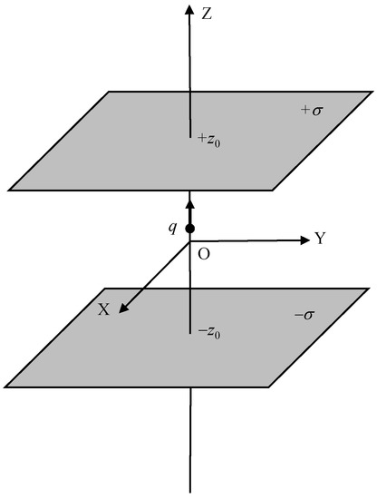
Figure 1.
Scheme of the problem to study.
4.1. Relativistic Solution
According to the conventional framework (the Maxwell–Lorentz and SRT framework), there is no electric field outside the capacitor, but inside there is a uniform electric field given by , which means that there is a voltage difference between the two infinite plates given by .
Taking into account the law of energy conservation, the total mechanical energy of a particle of mass (m) and charge (q) can be expressed as
where the relativistic expression of kinetic energy is considered, being the velocity of the charge with respect to the chosen reference frame. Assuming that at the midpoint between the plates, , a charge (q), with mass (m) and zero initial velocity is placed, the energy at any z between 0 and z0 is expressed as
from which, isolating v, we obtain
It can be seen from this expression that no matter how high a value V0 might be, v cannot exceed the value of c (i.e., if , then ), in accordance with the postulations of the SRT.
The force felt by the test charge outside the capacitor would be zero, since there is no electric field outside. Inside the capacitor, however, the charge would feel a force given by
where a is the acceleration at which the charge would move rectilinearly, according to SRT [18].
4.2. Solution with the New Electrodynamics
In previous works [26,37], this problem was solved using Weber’s and Phipps’ electrodynamical potential energies. In both cases, it was found that the solution obtained did not guarantee the existence of an upper limit to the velocity, unless an expression for kinetic energy different from the Newtonian one, such as the relativistic expression or something similar, was used. In the same sense, to overcome the above drawback, in a previous work [27] by the author, the need to use effective potential energy, , was shown, so that
Applying this expression to Phipps’ potential energy yields to obtain the following effective potential energy,
Integrating this interaction energy for all fixed charges located on the capacitor plates, the following expression is obtained for the net potential energy of the test charge, q:
In the zone between the plates, , the conservation of energy requires that
where the new expression for the kinetic energy, given by Equation (27), is used, now being , because this is the velocity, relative to the centre of mass, in the direction of the resultant force acting on the charge (responsible for kinetic work), and , because the mass of the capacitor (which we can assume to be concentrated at its centre of mass) is much larger than that of the test charge.
By rearranging terms, Equation (67) can be rewritten as
which coincides exactly with the relativistic result given by Equation (60). Naturally, Equations (61) and (62) are also derived from this.
For the outer zone (), the conservation of energy translates into
which is simplified to
which is the same result that would be obtained assuming that the electric potential is constant in the zone outside the plates (it would not be the case if we integrate Phipps’ potential energy directly).
Although the new framework proposed here succeeds in reproducing the same result as that obtained using Maxwell–Lorentz and SRT, there are profound differences between the two approaches. In SRT, the reason for the existence of a limiting velocity is that if the particle velocity with respect to an inertial observer is v, as , we see that , so the particle acceleration tends to be zero, giving a limiting velocity, even though the electric force does not cease. With the model proposed here, however, T does not tend to be infinity as , but it is the electric force (through the electrodynamic potential) that tends to be zero as , preventing subsequent acceleration. Thus, although the two models yield similar energetic results, there are profound metaphysical differences between them, and they cannot be considered equivalent. The advantage of this new electrodynamic route is that the simple space-time framework of Newtonian mechanics can still be used.
On the other hand, Phipps’ effective force, i.e., the force derived from Phipps’ effective potential energy, Equation (5), turns out to be
Integrating this elementary force over all the fixed charges on the capacitor plates, we find the following net force acting on the test charge, q. After integration we obtain
An alternative and faster way to find the force is to apply to the net potential energy, U, given by Equation (66).
Equating both branches of Equation (72) with Equation (34), considering and , we obtain two equalities. The first one is only valid whenever . The second one turns out to be
and inserting Equation (68) into Equation (73), after algebraic manipulation and simplification, we obtain
This result is in line with the prediction of the Maxwell–Lorentz and SRT framework, Equation (63).
4.3. Why Does the Effective Potential Energy Work?
It is not obvious why the calculation in the previous section should use the effective potential energy and not the potential energy directly, as in the case of the interaction of two charges. Some possible options were discussed in the paper [27]. The reason may lie in the fact that in the capacitor problem it is necessary to integrate, in application of the superposition principle, and this, in the case of velocity-dependent potentials, could introduce additional complexity.
From a mathematical point of view, however, the mission of the effective potential energy seems clear: it allows to recover, after the integration process of the potential energy, a functional dependence on velocity similar to that of Phipps.
Assuming that the potential energies U and U* are given by
in the capacitor problem, in order to know the potential energy felt by the test charge, basically the following calculation has to be carried out: . Thus, if the objective is that, after the integration process required by the principle of superposition, the result is an expression with the same dependence on velocity as Phipps’ expression, then it must be fulfilled that
Deriving the last equation with respect to , it is found that
Additionally, operating
Thus, taking into account the definitions given in Equation (75) and Equation (76), it is concluded that
which coincides exactly with Equation (64).
Thus, the definition given for U* guarantees that, after the integration process which the superposition principle forces, functional dependence on the velocity of Phipps’ expression is recovered. The question is whether or not this effective potential energy, U*, is merely a mathematical subterfuge or hides some subtle physical meaning. We leave the study of this possibility for another paper.
5. Conclusions
In this work, it is shown that it is possible to derive together the expressions for Phipps’ electrodynamic potential energy and its corresponding kinetic energy on the basis of the principles of energy conservation and mass–energy equivalence. In the limit of low energies and low velocities, it is known that this potential energy becomes Weber’s potential energy, and it has now been proven that the new expression for kinetic energy becomes the classical Newtonian expression.
The sum of Phipps’ potential and new kinetic energies turns out to be equivalent to the sum of the Coulomb potential energy and the SRT kinetic energy. However, the equivalence ends there, because the new approach shares the space-time framework of classical Newtonian mechanics and not the relativistic space-time framework, or its Lorentz transformations.
With the new electrodynamic framework proposed in this work, the problem of two interacting charges, in radial or orbital relative motion, is tackled. For these studies, new expressions for linear momentum, angular momentum, force and kinetic energy are proposed which are shown to be reduced to Newtonian expressions in the limit of low velocities and low energy. All the results obtained are consistent with the existence of a limiting velocity of the value of c, and they are in agreement with the predictions obtained by the Maxwell–Lorentz and SRT framework.
However, the new framework proposed is not sufficient to solve the problem of the motion of a charge between the plates of a charged capacitor. In order to also guarantee the existence of a limiting velocity in this case, it is necessary to resort to the so-called ‘effective potential energy’, which has already been introduced in a previous work. Considering this concept, the capacitor problem can be successfully solved and the same result as that achieved from the Maxwell–Lorentz and SRT framework can be reproduced.
In general, it can be concluded that, in the elementary cases studied, the results of the energy analysis and the dynamic analysis obtained with this new electrodynamic framework and the Maxwell–Lorentz and SRT framework coincide, even though both theoretical models are not metaphysically equivalent. This work opens the door to the consideration that Phipps’ electrodynamic approach and the conventional approach (Maxwell–Lorentz and SRT) could be just two different ways to describe the same reality.
Funding
This research received no external funding.
Institutional Review Board Statement
Not applicable.
Informed Consent Statement
Not applicable.
Data Availability Statement
Not applicable.
Conflicts of Interest
The author declares no conflict of interest.
Abbreviations
| c | speed of light in a vacuum |
| q1, q2 | interacting charges |
| m1, m2 | masses of the interacting charges |
| μ | Reduced mass |
| ε0 | vacuum’s electric permittivity |
| r | separation distance between the two interacting charges |
| radial relative velocity | |
| radial relative acceleration | |
| angle (in polar coordinates) | |
| angular speed | |
| angular acceleration | |
| UC | Coulomb’s potential energy |
| UW | Weber’s potential energy |
| UP | Phipp’s potential energy |
| U, T, E | potential, kinetic and total energy |
| U* | effective potential energy |
| unit vector in the direction of | |
| unit vector in the transversal direction | |
| unit vector in the normal direction | |
| Weber’s force | |
| Phipp’s force | |
| F | modulus of a generic force |
| Weber’s effective force | |
| Phipp’s effective force | |
| (linear) momentum | |
| angular momentum | |
| γ | |
| γ0 | initial value of γ |
| α | |
| electric field between the plates of the capacitor | |
| V0 | voltage difference between the two plates of the capacitor |
| v | velocity of charge moving between the plates of the capacitor |
| m | mass of the moving charge |
| 2 z0 | distance separating capacitor plates |
Appendix A. Derivation of the Kinetic Energy for Orbital Motion
In Equation (45), the only non-zero component of the force is the component in , which is expressed as
On the other hand, the total velocity of the moving charge is expressed in polar coordinates as . As, in addition, , it follows that
Since the force is a central force, the angular momentum is conserved, so its time derivative must be zero, that is, . Applying this to Equation (44), which defines the angular momentum, we arrive at the following equation:
Inserting Equation (A3) into Equation (A2), we obtain
and hence,
Integrating the above,
where and . Calculating this equation, the following is finally obtained:
Appendix B. Proof That Is Parallel to
The velocity consists of a radial and a transversal component. Namely,
According to Equation (43), the momentum is given by
For to be parallel to , it is required that
which is not fulfilled in general. However, in the present case, where the force is central, from Equation (45), it is satisfied that
On the other hand, taking into account the definition of angular momentum, Equation (44), and that , also because the force is central, then
Comparing Equation (A11) and Equation (A12), Equation (A10) is obtained, which is exactly the necessary requirement for to be parallel to .
References
- Ampère, A.M. Mémoire Sur la Théorie Mathématique des Phénomenes Électrodynamiques, Uniquement Déduite de L’expérience; Academy Science: Paris, France, 1823; Volume 6, p. 175. [Google Scholar]
- Gauss, C.F. Zur Mathematischen Theorie der Elektrodynamischen Wirkung; Werke: Göttingen, Germany, 1867; Volume V, p. 602. [Google Scholar]
- Weber, W. Elektrodynamische Maassbestimmungen über ein Allgemeines Grundgesetz der Elektrischen Wirkung; Reprinted in Wilhelm Weber’s Werke; Springer: Berlin/Heidelberg, Germany, 1893; Volume 3, pp. 25–214. [Google Scholar]
- Riemann, B. Schwere, Elektrizität, und Magnetismus, C; Rümpler: Hannover, Germany, 1876; p. 327. [Google Scholar]
- Maxwell, J.C. A Treatise on Electricity and Magnetism; Dover: Mineola, NY, USA, 1954; Volume 2, Chapter XXIII. [Google Scholar]
- Weber, W. Electrodynamic Measurements—Sixth Memoir, Relating Specially to The Principle of The Conservation of Energy. Lond. Edinb. Dublin Philos. Mag. J. Sci. 1872, 43, 1–20. [Google Scholar] [CrossRef]
- Shalm, L.K.; Meyer-Scott, E.; Christensen, B.G.; Bierhorst, P.; Wayne, M.A.; Stevens, M.J.; Gerrits, T.; Glancy, S.; Hamel, D.R.; Allman, M.S.; et al. Strong loophole-free test of local realism. Phys. Rev. Lett. 2015, 115, 250402. [Google Scholar] [CrossRef] [PubMed]
- Hensen, B.; Bernien, H.; Dréau, A.E.; Reiserer, A.; Kalb, N.; Blok, M.S.; Ruitenberg, J.; Vermeulen, R.F.L.; Schouten, R.N.; Abellán, C.; et al. Loophole-free Bell inequality violation using electron spins separated by 1. 3 km. Nature 2015, 526, 682–686. [Google Scholar] [CrossRef] [PubMed]
- Assis, A.K.T. Weber’s Electrodynamics; Kluwer Academic Publishers: Dordrecht, The Netherlands, 1994. [Google Scholar]
- Baumgärtel, C.; Maher, S. Foundations of Electromagnetism: A Review of Wilhelm Weber’s Electrodynamic Force Law. Foundations 2022, 2, 949–980. [Google Scholar] [CrossRef]
- Papageorgiou, C.; Raptis, T. Fragmentation of Thin Wires Under High Power Pulses and Bipolar Fusion. AIP Conf. Proc. 2010, 1203, 955–960. [Google Scholar]
- Kühn, S. Experimental investigation of an unusual induction effect and its interpretation as a necessary consequence of Weber electrodynamics. J. Electr. Eng. 2021, 72, 366–373. [Google Scholar] [CrossRef]
- Smith, R.T.; Jjunju, F.P.; Maher, S. Evaluation of Electron Beam Deflections across a Solenoid Using Weber-Ritz and Maxwell-Lorentz Electrodynamics. Prog. Electromagn. Res. 2015, 151, 83–93. [Google Scholar] [CrossRef]
- Smith, R.T.; Maher, S. Investigating Electron Beam Deflections by a Long Straight Wire Carrying a Constant Current Using Direct Action, Emission-Based and Field Theory Approaches of Electrodynamics. Prog. Electromagn. Res. 2017, 75, 79–89. [Google Scholar] [CrossRef]
- Baumgärtel, C.; Smith, R.T.; Maher, S. Accurately predicting electron beam deflections in fringing fields of a solenoid. Sci. Rep. 2020, 10, 10903. [Google Scholar] [CrossRef]
- Baumgärtel, C.; Maher, S. A Charged Particle Model Based on Weber Electrodynamics for Electron Beam Trajectories in Coil and Solenoid Elements. Prog. Electromagn. Res. C 2022, 123, 151–166. [Google Scholar] [CrossRef]
- Baumgärtel, C.; Maher, S. Resolving the Paradox of Unipolar Induction—New Experimental Evidence on the Influence of the Test Circuit. Sci. Rep. 2022, 12, 16791. [Google Scholar] [CrossRef] [PubMed]
- Härtel, H. Unipolar Induction-a Messy Corner of Electromagnetism. Eur. J. Phys. Educ. 2020, 11, 47–59. [Google Scholar]
- Prytz, K.A. Meissner effect in classical physics. Prog. Electromagn. Res. 2018, 64, 1–7. [Google Scholar] [CrossRef]
- Assis, A.K.T.; Tajmar, M. Superconductivity with Weber’s electrodynamics: The London moment and the Meissner effect. Ann. Fond. Louis Broglie 2017, 42, 307–350. [Google Scholar]
- Tajmar, M.; Assis, A.K.T. Influence of Rotation on the Weight of Gyroscopes as an Explanation for Flyby Anomalies. J. Adv. Phys. 2016, 5, 176–179. [Google Scholar] [CrossRef]
- Lörincz, I.; Tajmar, M. Experimental Investigation of the Influence of Spatially Distributed Charges on the Inertial Mass of Moving Electrons as Predicted by Weber’s Electrodynamics. Can. J. Phys. 2017, 95, 1023–1029. [Google Scholar] [CrossRef]
- Weikert, M.; Tajmar, M. Investigation of the Influence of a field-free electrostatic Potential on the Electron Mass with Barkhausen-Kurz Oscillation. arXiv 2019, arXiv:1902.05419. [Google Scholar]
- Tajmar, M.; Weikert, M. Evaluation of the Influence of a Field-Less Electrostatic Potential on Electron Beam Deflection as Predicted by Weber Electrodynamics. Prog. Electromagn. Res. M 2021, 105, 1–8. [Google Scholar] [CrossRef]
- Phipps, T.E., Jr. Toward modernization of Weber’s force law. Phys. Essays 1990, 3, 414–420. [Google Scholar] [CrossRef]
- Assis, A.K.T.; Caluzi, J.J. A limitation of Weber’s law. Phys. Lett. A 1991, 160, 25–30. [Google Scholar] [CrossRef]
- Montes, J.M. On limiting velocity with Weber-like potentials. Can. J. Phys. 2017, 95, 770–776. [Google Scholar] [CrossRef]
- Schrödinger, E. Die Erfüllbarkeit der Relativitätsforderung in der klassischen Mechanik. Ann. Der Phys. 1925, 77, 325–336. [Google Scholar] [CrossRef]
- French, A.P. Special Relativity; W.W. Norton & Co.: New York, NY, USA, 1968. [Google Scholar]
- Caluzi, J.J.; Assis, A.K.T. A critical analysis of Helmholtz’s argument against Weber’s electrodynamics. Found. Phys. 1997, 27, 1445–1452. [Google Scholar] [CrossRef]
- Assis, A.K.T.; Caluzi, J.J. Charged particle oscillating near a capacitor. Galilean Electrodyn. 1999, 10, 103–106. [Google Scholar]
- Li, Q. Extending Weber’s Electrodynamics to High Velocity Particles. Int. J. Magn. Electromagn. 2022, 8, 40. [Google Scholar]
- Wesley, J.P. Selected Topics in Scientific Physics; Benjamin Wesley Publisher: Blumberg, Germany, 2002; pp. 99–100. [Google Scholar]
- Önem, C. The Solutions of the Classical Relativistic Two-Body Equation. Turk. J. Phys. 1998, 22, 107–114. [Google Scholar]
- Assis, A.K.T.; Clemente, R.A. The ultimate speed implied by theories of Weber’s type. Int. J. Theor. Phys. 1992, 31, 1063–1073. [Google Scholar] [CrossRef]
- Clemente, R.A.; Assis, A.K.T. Two-body problem for Weber-like interactions. Int. J. Theor. Phys. 1991, 30, 537–545. [Google Scholar] [CrossRef]
- Caluzi, J.J.; Assis, A.K.T. An analysis of Phipps’s potential energy. J. Frankl. Inst. 1995, 332, 747–753. [Google Scholar] [CrossRef]

Disclaimer/Publisher’s Note: The statements, opinions and data contained in all publications are solely those of the individual author(s) and contributor(s) and not of MDPI and/or the editor(s). MDPI and/or the editor(s) disclaim responsibility for any injury to people or property resulting from any ideas, methods, instructions or products referred to in the content. |
© 2023 by the author. Licensee MDPI, Basel, Switzerland. This article is an open access article distributed under the terms and conditions of the Creative Commons Attribution (CC BY) license (https://creativecommons.org/licenses/by/4.0/).